12] A. Economides and J. Silvester. Optimal Routing in a Network with Unreliable Links. ... 19] D. Johnson. NSFnet Report. In Proc. of the Nineteenth Internet ...
Type-of-Service Routing in Dynamic Datagram Networks� Ibrahim Matta, A. Udaya Shankar Institute for Advanced Computer Studies and Department of Computer Science University of Maryland College Park, Maryland 20742 CS-TR-3147 UMIACS-TR-93-95 October 1993
Abstract
We propose a new approach to achieving type-of-service (TOS) with adaptive next-hop routing in wide-area networks such as the Internet. We consider two tra�c classes, namely delay-sensitive and throughput-sensitive. In routing protocols such as OSPF and integrated IS-IS, each node has a di�erent nexthop for each destination and TOS. Traditionally, each node has a single FCFS queue for each outgoing link, and the next-hops are computed using link measurements. In our approach, we attempt to isolate the two tra�c classes by using two FCFS queues for each outgoing link, one for each TOS; the link is shared cyclicly between the two TOS queues. The next-hops for the delay-sensitive tra�c adapts to link delays of that tra�c. The next-hops for the throughputsensitive tra�c adapts to overall link utilizations. We compare our approach with the traditional approach using discrete-event simulation and Liapunov analysis (for stability of routes). The proposed approach o�ers lower end-to-end delay to the delay-sensitive tra�c. A related property is that the routes for the delay-sensitive tra�c are more stable, i.e. less oscillations. An unexpected property is that the overall end-to-end delay is lower; this is because the link utilization metric makes the throughput-sensitive tra�c move away to under-utilized routes, thus isolating the two tra�c classes and yielding a better overall network performance.
Categories and Subject Descriptors: C.2.1 [Computer-Communication Networks]: Network Ar-
chitecture and Design|packet networks; store and forward networks; C.2.2 [Computer-Communication Networks]: Network Protocols|protocol architecture; C.2.m [Routing Protocols]; C.4 [Performance of Systems]: modeling techniques; performance attributes; F.2.m [Computer Network Routing Protocols];
This work is supported in part by ONR and DARPA under contract N00014-91-C-0195 to Honeywell and Computer Science Department at the University of Maryland, and by National Science Foundation Grant No. NCR 89-04590. The views, opinions, and/or ndings contained in this report are those of the author(s) and should not be interpreted as representing the o�cial policies, either expressed or implied, of the Defense Advanced Research Projects Agency, ONR, the U.S. Government or Honeywell. Computer facilities were provided in part by NSF grant CCR-8811954. �
Contents
1 Introduction 2 Discrete-Event Simulations
1 3
3 Stability Analysis
7
2.1 Model : : : : : : : : : : : : : : : : : : : : : : : : : : : : : : : : : : : : : : : : : : : : 2.2 Observations : : : : : : : : : : : : : : : : : : : : : : : : : : : : : : : : : : : : : : : :
3 5
3.1 Model : : : : : : : : : : : : : : : : : : : : : : : : : : : : : : : : : : : : : : : : : : : : 7 3.2 Liapunov Function Method : : : : : : : : : : : : : : : : : : : : : : : : : : : : : : : : 10
4 Conclusions and Future Work
17
i
1 Introduction With the increasing diversity of network applications, it has become crucial for networks to o�er varying types of service, referred to as TOS, e.g. low delay, high throughput, etc. This means that a network's routing protocol should be able to determine appropriate routes for each TOS. Most of the design and analysis work on TOS assumes connection-oriented (or virtual-circuit) routing (e.g. [31, 14, 9, 36, 13]). This paper is concerned with achieving TOS using next-hop (datagram) routing on wide-area store-and-forward networks. Next-hop routing, which is currently used in the Internet, is a simple and robust way to do adaptive routing. Next-hop TOS routing is done as follows. Each node maintains for each destination node and TOS, a neighboring node id, referred to as the next-hop. Every data packet header contains its destination id and the TOS requested by the application. When a node receives a data packet, it forwards the packet to the next-hop for the packet's destination and TOS. The objective of the routing protocol is to choose next-hops so that the resulting routes satisfy the requested TOS. The quality of service o�ered by a route depends on the tra�c through its links, which depends on the time-varying external load. Consequently, a routing protocol must monitor link tra�c changes and adapt its next-hops. To do this, each node maintains for each outgoing link and TOS, a dynamic link cost, which is updated regularly according to the tra�c owing through the link. This link cost information is regularly disseminated to nodes of the network. Based on received link cost information, each node maintains and regularly updates its next-hop for each destination and TOS. The IP layer of the Internet Protocol suite speci es di�erent TOS [2]. Among them are the minimum delay service required for example by interactive tra�c or real-time tra�c (e.g. audio), and the maximum throughput service required for example by bulk transfers such as network mail or FTP. Routing protocols such as the Internet OSPF [29] and the OSI IS-IS [7] provide separate next-hops for each TOS. However, the TOS mechanism has been so far of little use, and little is known on how well it would work in practice. In addition, many current routing protocols use static link costs1 (which respond only to failures and recoveries). To our knowledge, only one approach to adaptive TOS routing has been proposed [16]. This approach, henceforth called TOS1, considers two TOS: low delay and high throughput. It uses measured link delays as the link costs for the delay-sensitive tra�c2 (delay-based routing). It uses link utilizations (or equivalently available link 1 Typically con gured by the network administrator. 2 Delay-sensitive tra�c refers to the tra�c requiring low delay service.
tra�c requiring high throughput service.
1
Throughput-sensitive
tra�c refers to the
capacities) as the link costs for the throughput-sensitive tra�c (utilization-based routing). In TOS1, each node maintains for each outgoing link, a single FCFS queue of data packets; that is, packets of every TOS share this queue. Reference [16] refers to simulation studies but does not present any quantitative results. Traditionally, link queueing disciplines have been of the FCFS type. It appears desirable to use a more structured queueing discipline that helps \isolate" the di�erent TOS classes, for example, by using a separate queue for each TOS class. This concept of isolating tra�c classes using structured queueing disciplines has been used recently in ow control studies, e.g. [10, 20, 6, 31, 13]. In this paper, we investigate the use of a structured queueing discipline with adaptive next-hop TOS routing.
Our approach We consider a simple two-queue link scheduling discipline, henceforth referred to as type-of-service queueing. We consider two TOS: low delay and high throughput. With type-of-service queueing, each node maintains two FCFS queues for each outgoing link, one for each type of service. The link bandwidth is allocated equally between the two queues in a round-robin fashion. (Type-ofservice queueing is similar to the recently proposed fair-queueing discipline [10], except that in fair-queueing, the link bandwidth is divided equally amongst the connections using the link, rather than the types of service.) For any link, the link cost for delay-sensitive tra�c is obtained by exponentially averaging the measured delay that is experienced by delay-sensitive packets only. The link cost for throughputsensitive tra�c is obtained by exponentially averaging the measured utilization of the link (i.e. accounting for both delay-sensitive and throughput-sensitive packets). Henceforth, we refer to our approach as TOS2. Our discrete-event simulations on a subset of the NSFNET-T1-Backbone topology show that TOS2 performs signi cantly better than TOS1 in a typical situation where the proportion of delaysensitive tra�c is small compared to the throughput-sensitive tra�c [19]. TOS2 not only yielded a lower end-to-end delay for delay-sensitive packets (as expected), but also a lower overall end-to-end delay (which is unexpected). We argue that this is because with TOS2, the routing is signi cantly improved as we exploited the scheduling structure of type-of-service queueing when calculating link costs. In particular, the routes of the two tra�c classes can be isolated with the delay-sensitive tra�c taking the low delay 2
routes, and the throughput-sensitive tra�c taking the under-utilized routes. This results in a better overall network performance. In fact, we nd that a non-TOS scheme, which does not distinguish between the two types of tra�c and applies utilization link cost to both, referred to as UTIL, performs signi cantly better than TOS1 at high load. To gain more insight into the system behavior with both TOS schemes (TOS1, TOS2), we analyzed in [26] a simple model of a single source-destination node pair connected by two (parallel) paths; the rst path representing low delay routes, and the second path representing high capacity routes. We viewed this system as a dynamical system [3]. We represented isolation by a stable state where all delay-sensitive tra�c stays on the rst path, and all throughput-sensitive tra�c stays on the second path. We applied the Liapunov function method, and derived stability theorems ignoring propagation delays. In this paper, we derive our stability results taking into account the propagation delays. We show that for certain parameter values, the isolation state provides the best delay performance for both tra�c classes. We also show that TOS2 has a larger stability region corresponding to isolation than TOS1.
Organization of the paper The paper is organized as follows. Section 2 describes our discrete-event simulation model and results. Section 3 presents our Liapunov stability analysis. Section 4 concludes the paper. Appendix I describes details of the simulations, including performance measures, scenarios, and plots. Appendix II contains details of some derivations and proofs.
2 Discrete-Event Simulations Our simulation studies were done with a discrete-event simulator, MaRS [1], which has been used for other studies of routing algorithms [33, 32]. In Subsection 2.1, we describe the simulation model. In Subsection 2.2, we present general observations about the results.
2.1 Model Regarding the physical network, we consider the \East coast" subset of the NSFNET-T1-Backbone. Figure 1 illustrates the topology. Link propagation delays in milliseconds are indicated.
3
5 7
5 8 5
4
8
14
9
Figure 1: The \East coast" subset of the NSFNET-T1-Backbone (7 nodes, 9 bidirectional links). We have two versions: a low-speed version (with NSFNET-T1 parameters) and a high-speed version. There are no link or node failures. All nodes have adequate bu�er space for bu�ering packets awaiting processing and forwarding. Regarding link scheduling, we consider two disciplines for the scheduling of data packets over the links: FCFS and type-of-service queueing. Both TOS1 and UTIL use FCFS. TOS2 uses type-ofservice queueing. In all schemes, routing packets have priority over data packets; i.e. data packets can be scheduled for transmission only if there are no routing packets present. Regarding routing, we consider a link-state algorithm like the SPF (Shortest Path First) algorithm used in the ARPANET [27] and OSPF (Open SPF) used in the Internet [29]. Each node maintains a time-varying cost (explained below) for each outgoing link and TOS. Each node also maintains a view of the network topology, with a cost for each TOS and link in the network. To keep these views up-to-date, each node regularly broadcasts the link costs of its outgoing links to all other nodes using ooding3 . As a node receives this information, it updates its view of the network topology and applies Dijkstra's shortest path algorithm [11] to choose its next-hop for each destination and TOS. The method used to compute link costs for each TOS depends on the link scheduling discipline. In all cases, each node's outgoing link costs are updated regularly. A link cost is always a simple moving average of a \raw cost", which is some measure of current link tra�c. In the TOS schemes, each node maintains the following two raw-costs for each outgoing link: � RawUtilization: percentage of time the communication channel is busy transmitting a packet; and � RawDelay: In TOS1, this is the average packet delay (queueing, transmission, and propaga3 A node sends link cost information to its neighbors, they forward this information to their neighbors and so on.
4
tion) in milliseconds as experienced by all data packets. In TOS2, this is the average delay in milliseconds as experienced by delay-sensitive packets only. Let LinkCost(D) and LinkCost(T ) denote the link cost for delay-sensitive and throughputsensitive tra�c, respectively. Then at the end of each update interval, they are updated as follows:
LinkCost(D) := b � RawDelay + (1 ? b) � LinkCost(D) LinkCost(T ) := b � RawUtilization + (1 ? b) � LinkCost(T ) where the constant b � (0; 1). Recall that UTIL does not use any TOS facility. The utilization metric is used to compute one next-hop for every destination at each network node (i.e. LinkCost(T ) is used for all tra�c). With a utilization-based link cost metric, it seems natural to de ne the cost of a path as the minimum available link bandwidth (highest link utilization) of the links along the path. However, the more links there are with only a small amount of available bandwidth along a path, the more likely that using this path will tie up more resources leading to congestion [8]. In fact, we found that such path cost metric leads to large routing oscillations and instability (even at low workload). Therefore, we set the path cost metric to the sum of the link costs along the path from the source node to the destination node and use Dijkstra's shortest path algorithm as in [17]. Regarding the workload, it is de ned in terms of hsource node; destination nodei pairs. In each pair, the source produces data packets to be delivered to the destination. A source produces data packets according to a packet-train model [18]. The workload consists of two parts, a delay-sensitive workload and a throughput-sensitive workload. For both parts, we use a uniform distribution of source-destination pairs over the nodes of the network. Let parameter U (D) (U (T )) denote the average number of source-destination pairs between every two nodes for delay-sensitive (throughputsensitive) tra�c. (We have also investigated skewed distribution of source-destination pairs, and obtained similar results.)
2.2 Observations In this subsection, we present general observations about the simulation results. Detailed descriptions of scenarios simulated (parameters settings, etc.) and plots of the observed performance measures are given in Appendix I. In every scenario, the system behaves in a manner typical of open queueing networks [23]. That is, the throughput is equal the workload as long as the workload is less than the system capacity; 5
for workload higher than the system capacity the system is unstable. With increasing workload, the delay increases at rst slowly until a point where the system starts becoming saturated; we refer to this point as the saturation point. Further increase in the workload beyond this point causes the delay to increase dramatically (with increasing rate) until the system becomes unstable. Fixing U (D) and varying U (T ) in a range where the delay-sensitive tra�c constitutes almost 25%-30% of the total tra�c, we found that TOS2 performs signi cantly better than TOS1 with respect to delays; TOS1 reaches saturation sooner. (See Figure 2.) Delay
TOS1
UTIL
TOS2
U (T)
Figure 2: A generic plot. Delay versus U (T ) for a xed U (D). Our explanation is as follows: It is well known that delay-based routing does not perform well at high load when queueing delay is a signi cant part of measured link delay, which consists of queueing, transmission, and propagation delays [21, 17, 5]. This is mainly because from the classical delay-utilization curve, around saturation, a small increase in utilization corresponds to a large increase in link delay. This dramatic change can result in the link becoming unattractive and thus being avoided by all delay-sensitive sources. Consequently, at the next routing update the link reports a very low cost and becomes attractive again. This leads to oscillatory behavior, which in turn degrades performance [21]. This is the case with TOS1 due to the use of the FCFS link scheduling discipline. In TOS2, because delay-sensitive packets have a lower queueing delay under type-of-service queueing [10], the measured link delay becomes dominated by transmission and propagation delays. Thus, the reported delay link costs do not change dramatically and the delay metric remains a good indicator of expected link delay after updating the routes [21]. This improves the performance of delay-based routing of delay-sensitive packets and results in more stable routes for that tra�c class. Meanwhile, the link utilization metric makes the throughput-sensitive tra�c move away from the 6
delay-sensitive tra�c, taking the under-utilized routes. This has the e�ect of isolating the two tra�c classes, resulting in a better overall network performance. Intuitively, isolation is desirable since otherwise it becomes more likely that both tra�c classes will move away from a highly loaded link (i.e. with high delay and utilization) at the same routing update. Such simultaneous tra�c shifts degrade the overall performance, and in particular result in a higher delay and network under-utilization. Ignoring low values of U (T ), UTIL also provides lower delays than TOS1. However, UTIL performs worse than TOS2 over the whole range of U (T ). This is expected, since the utilizationbased metric does not necessarily result in minimum delay routes (especially at light load) [21].
3 Stability Analysis In this section, we consider a simple network model to gain more insight into the complicated behavior we observed in our simulation experiments. We derive stability conditions for the routes of the two tra�c classes under both TOS schemes (TOS1, TOS2). In Subsection 3.1, we give the model. In Subsection 3.2, we apply the Liapunov function method to analyze stability.
3.1 Model We model a network by a node S sending tra�c to node D along two paths. Path 1 represents low delay routes, and path 2 represents high capacity routes. Path i (i = 1; 2) has propagation delay Pi time units and average transmission capacity Ci packets/time unit.4 There are N delay-sensitive connections, and M throughput-sensitive connections from S to D. For every connection, packets originate at S according to a Poisson process, and without loss of generality we assume an arrival rate of 1 packet/time unit. At any instant, we describe the state of the network by the tuple (x; y ), where x is the number of delay-sensitive connections on path 1, and y is the number of throughput-sensitive connections on path 1. To model routing updates, we use a discrete-time ow approach as in [4]. We assume that (some or all) connections periodically update their routes to D every 4 time units, where 4 is long enough for the network to reach steady-state after a routing update. Routes, and hence the network state, are updated at discrete time instants (k + 1)4, k = 0; 1; 2; ���. Let (xk ; yk ) be the network state immediately after time k4. At an update instant (k + 1)4, we use steady-state 4 Thus we assume 1 + P1 < 1 + P2 and C2 > C1 . C1 C2
7
M=M=1 results [23] to estimate link costs based on (xk ; yk ). Using these link costs, routes are updated and consequently the new network state (xk+1 ; yk+1 ) is obtained. We denote by Ti;k+1 and �i;k+1 the delay and utilization cost of path i, respectively, at time (k + 1)4. Recall that for an M=M=1 queue with o�ered ow f and service rate �, the delay (queueing + service) is equal to 1=(� ? f ) provided that � > f (otherwise, the delay equals 1), and the utilization is equal to f=�. For TOS1, with a FCFS discipline at S , we can write the delay link costs as follows: T1;k+1 = C ? (x1 + y ) + P1 1 k k 1 T2;k+1 = C ? (�x + y� ) + P2 2
k
k
(1)
where x�k = N ? xk and y�k = M ? yk denote the number of delay-sensitive connections and the number of throughput-sensitive connections, respectively, on path 2. The utilization link costs are � = xk + yk 1;k+1
�2;k+1
C1 x � = k C+ y�k 2
(2)
The network state is updated using the costs of the two paths as follows:
8 < (1 ? �k ) xk xk+1 = : xk + �k x�k 8 < (1 ? �k ) yk yk+1 = : yk + �k y�k
if T2;k+1 < T1;k+1 otherwise if �2;k+1 � �1;k+1 otherwise
(3)
The parameter �k (0 < �k � 1) re ects the amount of tra�c rerouted. It can also be thought of as the degree of routing update synchronization at di�erent nodes. Unless otherwise indicated, we assume that �k is uniformly distributed over [�MIN ; �MAX ], where �MAX ? �MIN = 0:2, and 0:1 < �MAX +2 �MIN � 0:9. For TOS2, with a type-of-service queueing discipline at S , the two queues at an output link are correlated, which makes the analysis di�cult. A number of approximate solutions for such systems 8
(referred to as 1-limited polling systems) have been proposed. (See [35] for a good survey.) One common approach is to approximate the system by two loosely-coupled M=M=1 queues [28, 38]. The service rate of each queue depends on the utilization of the other queue. e� as the e�ective capacity available for the delay-sensitive tra�c on path i after time De ne Ci;k k4. We have e� � 0:5C Ci;k i
(4)
with the worst case occurring when the other queue is always not empty. Assuming each queue is M=M=1, we obtain the following (details in Appendix II): p 2 ( C 1 ? 0:5(yk ? xk )) + (C1 ? 0:5(yk ? xk )) ? 2C1xk e� C1;k = p 2 ( C ? 0 : 5(� y ? x � )) + (C2 ? 0:5(�yk ? x�k ))2 ? 2C2x�k k k C2e�;k = 2 2 (5) Thus we have the following delay link costs with type-of-service queueing: 1 T = +P 1;k+1
T2;k+1 =
C1e�;k ? xk C e�
1
�k 2;k ? x
1
+ P2 (6)
The utilization link costs are as de ned in (2). The network state is updated as in (3). We refer to the iteration de ned in (3) as I , i.e. (xk+1 ; yk+1 ) = I (xk ; yk ). I is a mapping from a set G into itself, where G = f(x; y ) : 0 � x � N ^ 0 � y � M g. The sequence of points (x1; y1 ); (x2; y2 ); : : : is called the trajectory of the system [24, 30]. The trajectory may or may not converge to a xed point (x�; y �), i.e. (x�; y �) = I (x�; y �). The convergence to a xed point indicates that the system stabilizes into a particular routing pattern. On the other hand, non-convergence indicates that the system oscillates between di�erent routing patterns (or has chaotic behavior). Note that I is not a continuous mapping, and well-known theorems for convergence requiring this property cannot be directly applied [22]. We represent isolation by a stable state where every delay-sensitive connection stays on path 1, and every throughput-sensitive connection stays on path 2. This is equivalent to say that our iterative method converges to the xed point (N; 0). In the next section, we rst derive su�cient 9
conditions for the system to reach isolation as a function of the starting state. (In a real network, the starting state would be the result of arrivals of new connections, departures of old connections, failure/recovery of links, etc.) We then obtain less re ned su�cient conditions for isolation, independent of the starting state.
3.2 Liapunov Function Method We use the Liapunov function method [30] to obtain su�cient conditions for stability and convergence to a xed point without actually solving the system equations. The basic idea is to nd a positive-de nite scalar function V (S), where S is the system state, such that its forward di�erence 4V (S) taken along a trajectory is always negative. V (S) is said to be a Liapunov function, and is regarded as a measure of the distance of the state S from the xed point. As time increases, V (S) decreases and nally shrinks to zero, i.e. the xed point is approached. It is more convenient to deal with the xed point (0; 0) rather than (N; 0). Thus, we de ne the network state by (�x; y ) instead of (x; y ). Then, the iteration I de ned in (3) becomes:
8< (1 ? �k ) x�k x�k+1 = : x�k + �k xk 8< (1 ? �k ) yk yk+1 = : yk + �k y�k
if T1;k+1 � T2;k+1 otherwise if �2;k+1 � �1;k+1 otherwise
(7)
Combining (1), (2), and (7), the system behavior with TOS1 is described by the following:
x�k+1 = (1 ? �k ) x�k + �k N �k yk+1 = (1 ? �k ) yk + �k M k (8) where
8 1 1 < 0 C1?N +(� x ? y ) + P1 � C2 ?M ?(� xk ?yk ) + P2 k k �k = : 1 otherwise 8 M +(�xk?yk ) N ?(�xk?yk ) 0 for all (�x; y) 6= (0; 0) and V (0; 0) = 0, then V (�x; y) is positive de nite. The forward di�erence 4V (�xk ; yk ) is computed as follows. 4V (�xk ; yk) = V (�xk+1; yk+1) ? V (�xk ; yk ) = ((1 ? �k ) x�k + �k N �k )2 + ((1 ? �k ) yk + �k M k )2 ?(�x2k + yk2) = ?[1 ? (1 ? �k )2 ] x�2k ? [1 ? (1 ? �k )2] yk2 + (�k N �k )2 + (�k M k )2 +2(1 ? �k ) �k N x�k �k + 2(1 ? �k ) �k M yk k
(12)
Consider a point (�xk ; yk ) � D1 ? f(0; 0)g. Then �k = k = 0. From equation (12), since 0 < [1 ? (1 ? �k )2] � 1, we have 4V (�xk ; yk ) < 0. (This is true regardless of the randomness of �k .) Substituting �k = k = 0 in equations (8), we get x�k+1 ? yk+1 = (1 ? �k )(�xk ? yk ). Consider the case where x�k ? yk < 0. Since 0 � (1 ? �k ) < 1, we have C1 ?N +(�x1k+1 ?yk+1 ) + P1 < 1 1 1 1 C1 ?N +(�xk ?yk ) + P1 , and C2 ?M ?(�xk ?yk ) + P2 < C2 ?M ?(�xk+1 ?yk+1 ) + P2 . Hence, since C1 ?N +(�xk ?yk ) + P1 � C2 ?M ?1(�xk ?yk ) + P2, we see that C1 ?N +(�x1k+1 ?yk+1 ) + P1 � C2 ?M ?(�x1k+1 ?yk+1 ) + P2 . 1 1 Now, consider the case where x�k ? yk > 0. We have C1 ?N +(� xk ?yk ) + P1 < C1 ?N + P1 , and 1 1 1 1 C2 ?M + P2 < C2 ?M ?(�xk ?yk ) + P2 . Since 0 � (1 ? �k ) < 1, and C1 ?N + P1 � C2 ?M + P2 from equation (10), we see that C1 ?N +(�x1k+1 ?yk+1 ) + P1 � C2 ?M ?(�x1k+1 ?yk+1 ) + P2 . ?yk+1 ) � N ?(�xk+1 ?yk+1 ) . Therefore, (�x ; y ) � D , and � = Similarly, we see that M +(�xk+1 k+1 k+1 1 k+1 C2 C1 k+1 = 0. Consequently, starting at any point in D1, the trajectory stays inside D1 approaching the origin (as shown in Figure 3).
End of Proof
From lemma 3.1 and the Liapunov stability theory [30], we have the following theorem:
Theorem 3.1 For TOS1, any starting state in D1 (the shaded area in Figure 3) leads to the origin,
regardless of the values of �k .
The region D1 is called domain of attraction corresponding to the origin [3, 22] because it constitutes a set of starting states for which the iteration converges to the origin. In D1 , the iteration is said to be a contraction, since V (�xk+1 ; yk+1 ) < V (�xk ; yk ) for all (�xk ; yk ) 6= (0; 0) along the trajectory. It is important to observe that the domain of attraction contains all the system states for which T1 � T2 and �2 � �1 . Also, note that starting at any point in D1, �k = k = 0 for all (�xk ; yk ) along the trajectory. 12
With TOS2, the system behavior is described by the same di�erence equations (8) except that �k is de ned as 8 >< 0 if e� 1 + P1 � e�1 + P2 C1;k ?N +�xk C2;k ?x�k �k = > : 1 otherwise At the xed point, xk ! N; x�k ! 0, yk ! 0; y�k ! M . Then, from equations (5), we have C2e�;k ! C2 ? 0:5M , and C1e�;k ! C1. For equations (8) to be satis ed at the xed point, �k ! 0 and k ! 0. Then necessary conditions for convergence to the origin are: 1 1 C1 ? N + P1 � C2 ? 0:5M + P2
M N C2 � C1
(13)
As we have done with TOS1, we want to show that V (�x; y ), de ned in (11), is a Liapunov function in some region around the origin. Call this region D2 . The goal is to show that starting at any point in D2, �k = k = 0 for all (�xk ; yk ) along the trajectory. 1 + P1 � C e�1?x� + P2 implies �k = 0. M +(�Cxk2?yk ) � N ?(�xCk1?yk ) implies k = 0. C e� ?N +�x k
1;k
2;k
k
e� are hard to work with, we try to nd simpler expressions, say Because the expressions for Ci;k simp , such that 1 1 1 1 Ci;k e� ?N +�x + P1 � C simp ?N +�xk + P1 , and C simp ?x�k + P2 � C e� ?x� + P2 (then C1;k k 1;k 2;k 2;k k 1 +P1 � C simp1 ?x� +P2 implies �k = 0). We would then de ne D2 = f(�x; y ) : C simp1?N +�x + C simp ?N +�x 1;k
k
2;k
k
M +(�x?y) C2
1
N ?(�x?y) C1
� ^ 0 � x� � N ^ 0 � y � M g, and attempt to show P1 � C simp ?x� + P2 ^ 2 that V (�x; y ), de ned in (11), is a Liapunov function in D2 . To do this, we need an upper bound on C2e�;k , and a lower bound on C1e�;k . From equations (5), we see that C2e�;k � C2 ? 0:5(�yk ? x�k ). We could not nd an appropriate lower bound on C1e�;k . So we made the approximation C1e�;k � C1 ? 0:5yk (the accuracy of this is discussed below). x?y) N ?(�x?y) ^ We thus have D2 = f(�x; y ) : (C1 ?0:51y)?N +�x + P1 � (C2 ?0:5(�1y?x�))?x� + P2 ^ M +(� C2 � C1 0 � x� � N ^ 0 � y � M g. Figure 4 depicts this region. 1
Lemma 3.2 Assuming C1e�;k � C1 ? 0:5yk, V (�x; y) is a Liapunov function in D2. The proof of the above lemma is similar to the proof of Lemma 3.1, and is given in Appendix II. From lemma 3.2 and the Liapunov stability theory [30], we have the following theorem:
Theorem 3.2 For TOS2, assuming C1e�;k � C1 ? 0:5yk, any starting state in D2 (the shaded area in Figure 4) leads to the origin, regardless of the values of �k .
13
1 0.5 C1 - x
+ P1 =
1 _ _ + P2 ( C + 0.5 x ) _ x 2
y
Domain of attraction D2 M 1
( C1 - 0.5 y ) - x =
+ P1 1
( C 2 _ 0.5 ( y _ x )) _ x
+ P2 x N x+y C 2
=
x+y C 1
Figure 4: Domain of attraction for TOS2.
E�ect of �k on system behavior The domains of attraction we have just found (cf. Theorems 3.1 and 3.2) are not the largest, i.e. there may be points outside the domains which lead to the origin. This depends on the values of �k . In particular, the domains are indeed largest for high enough values of �k . On the other hand, they are not for small values of �k . The following theorem shows this for TOS1. The proof is given in Appendix II.
Theorem 3.3 For TOS1, starting at any point in area A or area B (Figure 3), the following
hold: (i) If �MIN > max( NM?+LN1 ; MM++LN2 ) then the iteration does not converge to the origin and locks into a limit cycle oscillating between states in areas A and B. (ii) If �MAX � min( LN2 ; ?ML1 ) then the iteration converges to the origin. where p H S ? 2 + (H S ? 2)2 + 4 H [H (C1 ? N ) (C2 ? M ) + S ] L1 = 2H H = P1 ? P2 S = C2 ? M ? C 1 + N L2 = C2CN ?+ CC1M 1 2
14
Theorem 3.3 indicates that for high enough values of �k , the system may not converge to isolation, and rather oscillates with both tra�c classes shifting simultaneously at each routing update. Such simultaneous tra�c shifts result in a bad performance, i.e. higher delay and network under-utilization. This e�ect increases as �k increases. (In practice, �k depend on several factors, and can be quite high [15].) Consider the simple case where �k = 1, for all k. It can be seen that isolation, whenever possible5 , provides the optimal performance for both tra�c classes [12]. In this case, we are constrained to use a single path for each tra�c class. Thus, in order to maximize the throughput of the throughput-sensitive tra�c, we should send its packets over the maximum capacity link, i.e. path 2. Then, in order to minimize the packet delay of the delay-sensitive tra�c, we should send its packets over the minimum packet delay link, i.e. path 1. Note that routing the delay-sensitive tra�c (also) on path 2 would result in a higher delay compared to the delay of (the unused) path 1. Note that the above result agrees with our argument about the bene ts of isolation, which was made in Subsection 2.2. Referring to Figures 3 and 4, we can conclude that for high enough �k , TOS2 has a larger domain of attraction corresponding to isolation than TOS1. This conclusion is not a�ected by our approximation C1e�;k � C1 ? 0:5yk , which was made in Theorem 3.2 for TOS2. In fact, it can be shown that C1e�;k � C1 ? 0:5yk . Regardless of that, we found that our approximation is only slightly optimistic. In particular, our monte-carlo simulations [26] show that starting at any point in D2 satisfying 0:5C1?1 N +�x + P1 � (C2 +01:5�x)?x� + P2 , the iteration indeed leads to the origin. Those points also satisfy (C1 ?0:51y)?N +�x + P1 � (C2 ?0:5(�1y?x�))?x� + P2 . This is because (C1 ?0:51y)?N +�x + P1 � 1 1 1 0:5C1 ?N +� x + P1 (with equality occurring when y = C1), and (C2 +0:5�x)?x� + P2 � (C2 ?0:5(�y?x�))?x� + P2. Some points in D2 not satisfying 0:5C1 ?1 N +�x + P1 � (C2 +01:5�x)?x� + P2 may not, however, lead to the origin. Such points constitute a small part of D2, and hence the approximation does not a�ect our conclusion that TOS2 has a larger domain of attraction corresponding to isolation. In particular, isolation occurs for higher values of y0 with TOS2 than with TOS1. Theorem 3.3 also indicates that for small enough values of �k , the system reaches isolation for all starting states and for all system con gurations satisfying the necessary conditions for isolation. Figure 5 depicts the load region, i.e. values of (N; M ), de ned by f(N; M ) : C1 1?N + P1 � C12 + P2 ^ N M C2 � C1 g. In this region, the necessary conditions for isolation, de ned in (10) and (13), for both 5 Which means that the necessary conditions to reach isolation are satis ed, i.e. the delay of path 1 carrying all delay-sensitive tra�c is less than or equal the delay of path 2 carrying all throughput-sensitive tra�c, with path 2's utilization being less than or equal path 1's utilization.
15
TOS1 and TOS2 are satis ed. This region thus de nes su�cient conditions to reach isolation for low enough �k for both TOS1 and TOS2. This is in agreement with our monte-carlo simulations obtained in [26] which also show that in this region, TOS2 gives much better transient performance, i.e. less oscillations and much faster convergence to isolation, than TOS1 (we have not yet been able to obtain transient measures analytically). M
=
C 2
M
N C 1
_ N = C1
1 1 C2
+ P2 _ P1
N
Figure 5: Load region for isolation for low enough �k for both TOS1 and TOS2.
Su�cient conditions independent of the starting state In Theorems 3.1 and 3.2, we derived su�cient conditions for the system to reach isolation as a function of the starting state. Now, using these theorems, we derive su�cient conditions for isolation independent of the starting state (and the values of �k ).6 Figure 6 depicts the load regions de ned by these su�cient conditions. M
M=
C2 N C1
region A (TOS2)
N + M
_ = C1
1 1 C
+ P2 _ P 1 2
region B (TOS1)
N region C
(TOS1, TOS2)
N = 0.5 C _ 1
1 1 C
+ P2 _ P 1 2
Figure 6: Load regions satisfying su�cient conditions for isolation independent of starting state. 6 These conditions were obtained in [26] (in a di�erent way) using a worst-case analysis.
16
Theorem 3.4
(i) For TOS1, the conditions N + M � C1 ? ( 1 +P12 ?P1 ) and CM2 � CN1 (regions B and C in C2 Figure 6) are su�cient for isolation (regardless of the starting state and the values of �k ). (ii) For TOS2, the corresponding conditions are N � 0:5C1 ? ( 1 +P12 ?P1 ) and CM2 � CN1 (regions A C2 and C in Figure 6).
The proof of Theorem 3.4 is given in Appendix II. Referring to Figure 6, we observe that for N less than 0:5C1 ? ( 1 +P12 ?P1 ) , TOS2 provides isolation (regardless of the starting state and the C2 values of �k ) for higher values of M than TOS1. This e�ect becomes more pronounced as C2 increases. Note that the conditions of Theorem 3.4 capture less information than the ones given by Theorems 3.1 and 3.2; i.e. there can be a system con guration that does not satisfy the su�cient conditions of Theorem 3.4, but still reaches isolation for some starting states or values of �k .
4 Conclusions and Future Work We found our proposed scheme (TOS2) very e�ective in providing lower end-to-end delays in a typical situation where the proportion of delay-sensitive tra�c is small compared to the throughputsensitive tra�c. This is because our scheme, by using a structured link queueing discipline (typeof-service queueing), reduces queueing delays for the delay-sensitive tra�c, hence improving the performance of delay-based routing (i.e. more stable routes) and providing this tra�c with low delay service. At the same time, the link utilization metric isolates the throughput-sensitive tra�c which takes the under-utilized routes, resulting in a better overall network performance. In general, we have shown how in an integrated services environment, routing with some form of non-FCFS scheduling support can provide signi cant performance improvement. In addition to simulation studies, we examined this behavior analytically. We obtained stability conditions using the Liapunov function method. We are currently extending our analysis to obtain transient characteristics such as convergence time. Analyzing the interactions between adaptive routing and other link queueing algorithms is an open research area. Future work is also needed to explore the interaction between all components of the congestion control problem, namely scheduling, ow control, and routing, on arbitrary network topologies. We are also investigating other approaches to adaptive next-hop TOS routing. One approach [39] is to maintain for delay-sensitive tra�c two minimum propagation delay routes and use the sec17
ondary route when the primary route becomes congested. This approach attempts to avoid the bad e�ect that queueing delay may have when it dominates measured link delay in delay-based routing. However, it is not clear how to split the delay-sensitive tra�c between the two available routes without causing severe oscillations while at the same time reducing queueing delays to provide a low delay service. Further research is needed to explore this area.
References
[1] C. Alaettino�glu, K. Dussa-Zieger, I. Matta, and A.U. Shankar. MaRS (Maryland Routing Simulator) { Version 1.0 User's Manual. Technical Report UMIACS-TR-91-80, CS-TR-2687, Department of Computer Science, University of Maryland, College Park, MD 20742, June 1991. [2] P. Almquist. Type of Service in the Internet Protocol Suite. Request for Comment RFC-1349, Network Working Group, July 1992. [3] K-H. Becker and M. Dor er. Dynamical Systems and Fractals. Cambridge University Press, 1989. [4] D. Bertsekas and R. Gallager. Data Networks, pages 297{333. Prentice-Hall, Inc., 1987. [5] D.P. Bertsekas. Dynamic Behavior of Shortest Path Routing Algorithms for Communication Networks. IEEE Transactions on Automatic Control, 27(1):60{74, February 1982. [6] J. Bolot and A.U. Shankar. A Discrete-Time Stochastic Approach to Flow Control Dynamics. In Proc. GLOBECOM '92, Orlando, Florida, December 1992. [7] R. Callon. Use of OSI IS-IS for routing in TCP/IP and Dual Environments. Request for Comment RFC-1195, Digital Equipment Corporation, December 1990. [8] R. Coltun. Virtual Circuit Routing Protocol Proposal. Internet Draft, March 1993. [9] D. Comer and R. Yavatkar. FLOWS: Performance Guarantees in Best E�ort Delivery Systems. In Proc. IEEE INFOCOM, Ottawa, Canada, pages 100{109, April 1989. [10] A. Demers, S. Keshav, and S. Shenker. Analysis and Simulation of a Fair Queueing Algorithm. In Proc. ACM SIGCOMM '89, pages 1{12, Austin, Texas, September 1989. [11] E. Dijkstra. A Note on Two Problems in Connection with Graphs. Numer. Math., 1:269{271, 1959. [12] A. Economides and J. Silvester. Optimal Routing in a Network with Unreliable Links. In Proc. IEEE INFOCOM '88, pages 288{297, August 1988. [13] D. Ferrari and D.C. Verma. Quality of Service and Admission Control in ATM Networks. Technical Report TR-90-064, International Computer Science Institute, Berkeley, California, December 1990. [14] D. Ferrari and D.C. Verma. A Scheme for Real{Time Channel Establishment in Wide{Area Networks. IEEE JSAC, 8(3):368{379, April 1990. [15] S. Floyd and V. Jacobson. The Synchronization of Periodic Routing Messages. In Proc. ACM SIGCOMM '93, San Francisco, California, September 1993. [16] M.L. Gardner, I.S. Loobeek, and S.N. Cohn. Type-of-Service Routing with Loadsharing. In Proc. GLOBECOM '87, Tokyo, Japan, November 1987. [17] D. Glazer and C. Tropper. A New Metric for Dynamic Routing Algorithms. IEEE Transactions on Communications, pages 360{367, March 1990. [18] R. Jain and S.A. Routhier. Packet Trains - Measurements and A New Model for Computer Network Tra�c. IEEE Journal on Selected Areas in Communication, SAC-4(6):986{995, September 1986. [19] D. Johnson. NSFnet Report. In Proc. of the Nineteenth Internet Engineering Task Force, pages 377{382, University of Colorado, National Center for Atmospheric Research, December 1990.
18
[20] S. Keshav, A. Agrawala, and S. Singh. Design and Analysis of a Flow Control Algorithm for a Network of Rate Allocating Servers. In Proc. IFIP WG 6.1/WG 6.4 Second International Workshop on Protocols for High-Speed Networks, pages 55{72, Palo Alto, CA, November 1990. [21] A. Khanna and J. Zinky. A Revised ARPANET Routing Metric. In Proc. ACM SIGCOMM '89, pages 45{56, September 1989. [22] D. Kincaid and W. Cheney. Numerical Analysis: Mathematics of Scienti c Computing. Brooks/Cole Publishing Company, 1991. [23] L. Kleinrock. Queueing Systems, volume I and II. New York: Wiley, 1976. [24] B. Kuo. Automatic Control Systems. Prentice-Hall, Inc., fourth edition, 1983. [25] Stephen S. Lavenberg. Computer Performance Modeling Handbook. Academic Press, 1983. [26] I. Matta and A.U. Shankar. On the Interaction between Gateway Scheduling and Routing. Technical Report CS-TR-3102, Department of Computer Science, University of Maryland, College Park, MD 20742, July 1993. To appear in the International Workshop on Modeling, Analysis and Simulation of Computer and Telecommunications Systems-MASCOTS '94. [27] J. McQuillan, I. Richer, and E. Rosen. The New Routing Algorithm for the ARPANET. IEEE Transactions on Communications, COM-28(5):711{719, May 1980. [28] N. Mitrou and D. Pendarakis. Cell-Level Statistical Multiplexing in ATM Networks: Analysis, Dimensioning, and Call-Acceptance Control w.r.t. QOS Criteria. In Queueing, Performance and Control in ATM (ITC-13), pages 7{12. J. Cohen and C. Pack (Editors). Elsevier Science Publishers B.V. (NorthHolland), 1991. [29] J. Moy. OSPF Version 2. RFC 1247, Network Information Center, SRI International, July 1991. [30] K. Ogata. Discrete-Time Control Systems. Prentice-Hall, Inc., 1987. [31] A. Parekh. A Generalized Processor Sharing Approach to Flow Control in Integrated Services Networks. Technical Report LIDS-TR-2089, Laboratory for Information and Decision Systems, Massachusetts Institute of Technology, 1992. [32] A.U. Shankar, C. Alaettino�glu, K. Dussa-Zieger, and I. Matta. Performance Comparison of Routing Protocols under Dynamic and Static File Transfer Connections. ACM Computer Communication Review, October 1992. [33] A.U. Shankar, C. Alaettino�glu, I. Matta, and K. Dussa-Zieger. Performance Comparison of Routing Protocols using MaRS: Distance-Vector versus Link-State. In Proc. ACM SIGMETRICS/PERFORMANCE, volume 20, pages 181{192, Newport, Rhode Island, June 1992. [34] H. A. Taha. Operations Research : An Introduction. Macmillan publishing Co., second edition, 1976. [35] H. Takagi. Queueing Analysis of Polling Models: An Update. In Stochastic Analysis of Computer and Communication Systems, pages 267{318. H. Takagi (Editor). Elsevier Science Publishers B.V. (NorthHolland), 1990. [36] H. Zhang and S. Keshav. Comparison of Rate{Based Service Disciplines. In Proc. ACM SIGCOMM '91, volume 21, pages 113{121, Zurich, Switzerland, September 1991. [37] L. Zhang. VirtualClock: A New Tra�c Control Algorithm for Packet Switching Networks. In Proc. SIGCOMM '90, pages 19{29, Philadelphia, Pennsylvania, September 1990. [38] W. Zhu and S. Chanson. Adaptive Threshold-based Scheduling for Real-Time and Non-Real-Time Tra�c. In Proc. IEEE RTSS '92, pages 125{135, Phoenix, Arizona, December 1992. [39] J. Zinky. Private Communication, 1992.
Appendix I: Simulation Details In this appendix, we describe the simulation parameters, and the performance measures. We also give details of simulated scenarios and plots. 19
Parameters All links have bandwidths of 1.5Mbit/sec for the low-speed version, and 100Mbit/sec for the highspeed version. Each node's outgoing link costs are updated regularly, with inter-update time uniformly distributed with mean 10 seconds [27] and standard deviation 1 second.7 The factor b, used in the link cost calculation, is 0.8.8 A data source is represented as a Markov chain with two states: a busy state and an idle state. In the busy state, the source produces a (geometrically distributed) number of data packets with some constant inter-packet generation time. The source then stays idle for an exponentially distributed duration before starting the transmission of the next train (burst) of packets. (This tra�c model has been used in many studies, e.g. [37].) Unless otherwise indicated, all sources have the following parameters: for the low-speed case, the data packet length equals 128 bytes, the inter{packet generation time is 150 msec, the average train size is 100 packets, and the average idle duration is 2 seconds (this corresponds to an average packet rate of about 0.006 packet/msec.); for the high-speed case, the data packet length is 5000 bytes, the inter{packet generation time is 50 msec, the average train size is 1000 packets, and the average idle duration is 2 seconds (this corresponds to an average packet rate of about 0.02 packet/msec.).
Performance Measures We consider average measures of throughput, delay and load. An average measure is based on statistics collected over a large measurement interval, which is the duration of the simulation except for an initial \startup interval" (to eliminate transient e�ects due to empty initial network). Thus: � Throughput. Total number of data bytes received at destinations during the measurement interval divided by the length of the measurement interval. � Delay. Total delay of all data packets received at destinations during the measurement interval divided by the number of those data packets, where delay of a data packet is de ned to be the time di�erence between sending a packet and receiving it at the corresponding destination. � Data Load. Fraction of the network capacity, i.e. sum of all link capacities, used by data packets during the measurement interval. � Throughput(T). Total number of data bytes received at destinations for the throughputsensitive tra�c during the measurement interval divided by the length of the measurement interval. � Delay(D). Total delay of all delay-sensitive data packets received at destinations during the measurement interval divided by the number of those data packets. 7 Update intervals at di�erent nodes are independent. 8 We chose the factor 0.8 after experimenting with other values. A small value such as 0.5 makes the routing
algorithm adapt slowly. Whereas a high value such as 1.0 may result in an unstable behavior.
20
Results Here, we present details of scenarios simulated along with plots of the observed (steady{state) performance measures, namely throughput, delay , throughput(T ), delay (D), and data load. In our simulations, 95% con dence intervals were computed using the method of independent replications [25, 34]. In particular, a measure, say x, is obtained as x1 +x2 +n ���+xn , where the x1 ; x2; : : :; xn are the measures obtained using the di�erent independent simulation runs. In all cases, the size of the con dence intervals is less than 2% of the mean. We now present our simulation results. Although we show results only for uniform workload, we obtained similar results for the skewed workload we investigated. We also obtained similar results for workload that has di�erent parameters for each tra�c type. In case (C ) below, we consider a smaller packet size for the delay-sensitive sources, namely 64 bytes rather than 128 bytes. We have scaled the delay plots for clarity, so delay values higher than 100 milliseconds are not shown.
(A) Low-speed, varying U(T), xed U(D), equal packet sizes. Figure 7 shows delay (D) and delay versus U (T ) in the range 20 to 26, for a xed U (D) = 8. The delay-sensitive tra�c constitutes almost 25% of the total tra�c. Ignoring di�erences at low values of U (T ), TOS1 performs the worst, becoming saturated around U (T ) = 22 (corresponding to almost 60% data load). Interestingly, UTIL which does not use any TOS facility performs better than TOS1. TOS2 performs the best. At U (T ) = 24, UTIL's delay is 53% higher than TOS2's, and TOS1's delay is 1322% higher than TOS2's. Note that UTIL performs worse than TOS2 over the whole range of U (T ). At low values of U (T ), UTIL performs the worst. At U (T ) = 20, UTIL has about 32% higher delay than both TOS2 and TOS1. Figure 8 shows data load, throughput(T ) , and throughput versus U (T ). Observe that the data load for TOS1 increases as TOS1 becomes saturated. This indicates the use of longer routes, and consequently higher delay. Both throughput(T ) and throughput increase linearly with the workload, and they are the same for all schemes. This shows that the system is stable for all schemes.
(B) High-speed, varying U(T), xed U(D), equal packet sizes. Figure 9 shows delay (D) and delay versus U (T ) in the range 8 to 18, for a xed U (D) = 4. The delay-sensitive tra�c constitutes almost 25% of the total tra�c. As observed in the low-speed case (A), ignoring di�erences at low values of U (T ), TOS2 performs the best, followed by UTIL, and then TOS1. TOS1 reaches saturation sooner, around U (T ) = 16 (corresponding to a data load of almost 61%). TOS1 has about 758% higher delay than TOS2 at U (T ) = 18. Note that for the same data load, the di�erence in delay is less signi cant than in case (A). This is due to the fact that in a high-speed network, queueing delay is less signi cant due to small transmission times. 21
For example, in the high-speed network, transmission time of the 5000-byte data packet on the 100Mb/s link is 0.0004 sec. Whereas in the low-speed network, transmission time of the 128-byte data packet on the 1.5Mb/s link is 0.7 sec. This fact reduces the e�ect of bad oscillations inherent in delay-based routing when queueing delays are signi cant. Figure 10 shows data load, throughput(T ) and throughput versus U (T ). Again, as in case (A), throughput(T ) and throughput increase linearly with the workload for all schemes. Henceforth, we do not show plots for throughput. We also do not show plots for UTIL since the utilization-based metric, as we have observed, does not necessarily result in minimum delay routes.9
(C) Low-speed, varying U(T), xed U(D), unequal packet sizes. Figure 11 shows delay (D) and delay versus U (T ) in the range 16 to 24, for a xed U (D) = 16. The delay-sensitive tra�c constitutes almost 28% of the total tra�c. As observed in (A), TOS2 performs better than TOS1. TOS1 reaches saturation sooner, around U (T ) = 18 (corresponding to a data load of almost 55%). TOS1 has about 1800% higher delay than TOS2 at U (T ) = 20. Figure 12 shows data load versus U (T ). Observe that TOS1 reaches saturation at a data load which is smaller than in (A). This is because here delay-sensitive tra�c has smaller packet sizes, thus su�ering higher delays with TOS1.
Appendix II: Proofs and Derivations
Computation of e�ective capacities
Let's consider two queues QX and QY with arrival rates X and Y , respectively, equally sharing a link with capacity C . De ne CXe� and CYe� as the e�ective link capacity available for tra�c X and Y , respectively. Also, let nX and nY be the number of packets in QX and QY , respectively. Thus, CXe� = C � Prob[nY = 0] + 0:5C � Prob[nY > 0] CYe� = C � Prob[nX = 0] + 0:5C � Prob[nX > 0] Note that CXe� � 0:5C (CYe� � 0:5C ), with the worst-case occurring when QY (QX ) is always not empty. Assuming each queue is M=M=1, and substituting Prob[nX = 0] = 1 ? Prob[nX > 0] = 1 ? X=CXe� and Prob[nY = 0] = 1 ? Prob[nY > 0] = 1 ? Y=CYe� we obtain two equations inpthe two unknowns CXe� and CYe� . Solving them, we get 2 CXe� = (C?0:5(Y ?X ))+ (C2 ?0:5(Y ?X )) ?2CX CYe� = CXe� + 0:5(Y ? X ) 9 We have also studied a non-TOS scheme similar to UTIL except that it uses the delay metric rather than the utilization metric (i.e. LinkC ost(D) is used for all tra�c); however we do not show plots for it since it performed badly at heavy load, as expected.
22
Proof of Lemma 3.2
Consider a point (�xk ; yk ) � D2 ? f(0; 0)g. (C1 ?0:5y1k )?N +�xk + P1 � (C2 ?0:5(�yk1?x�k ))?x�k + P2 implies C e� ?1N +�x + P1 � C e�1?x� + P2 , and hence �k = 0. Let's rewrite (C1 ?0:5y1k )?N +�xk + P1 � k 1;k 2;k k 1 1 1 (C2 ?0:5(� yk ?x�k ))?x�k + P2 as C1 ?N +(�xk ?0:5yk ) + P1 � C2 ?0:5M ?0:5(�xk ?yk ) + P2 . Since �k = k = 0 then x�k+1 ? 0:5yk+1 = (1 ? �k )(�xk ? 0:5yk ), and x�k+1 ? yk+1 = (1 ? �k )(�xk ? yk ). Consider the case where x�k ? 0:5yk < 0. This implies that x�k ? yk < 0. Since 0 � (1 ? 1 1 1 �k ) < 1, we have C1 ?N +(�xk+1 ?0:5yk+1 ) + P1 < C1 ?N +(�xk ?0:5yk ) + P1 , and C2 ?0:5M ?0:5(�xk?yk ) + P2 < 1 1 1 C2 ?0:5M ?0:5(�xk+1?yk+1 ) + P2 . Hence, since C1 ?N +(�xk ?0:5yk ) + P1 � C2 ?0:5M ?0:5(�xk ?yk ) + P2 , we see 1 1 that C1 ?N +(�xk+1 ?0:5yk+1 ) + P1 � C2 ?0:5M ?0:5(�xk+1?yk+1 ) + P2. Now, consider the case where x�k ? 0:5yk > 0. In this case, either x�k ? yk > 0 or x�k ? yk < 0. First, consider the case where x�k ? 0:5yk > 0 and x�k ? yk > 0. We have C1 ?N +(�x1k ?0:5yk ) + P1 < C1 1?N + P1 , and C2 ?10:5M + P2 < C2 ?0:5M ?10:5(�xk?yk ) + P2 . Since 0 � (1 ? �k ) < 1, and C1 1?N + P1 � C2 ?10:5M + P2 1 1 from equation (13), we see that C1 ?N +(�xk+1 ?0:5yk+1 ) + P1 � C2 ?0:5M ?0:5(�xk+1?yk+1 ) + P2 . We also see that the latter inequality also holds for the case where x�k ? 0:5yk > 0 and x�k ? yk < 0. Therefore, since in all cases, (C1 ?0:5yk+11 )?N +�xk+1 + P1 � (C2 ?0:5(�yk+1 ?1 x�k+1 ))?x�k+1 + P2 then M +(�xk+1 ?yk+1 ) � N ?(�xk+1 ?yk+1 ) . 1 1 e� ?N +�xk+1 + P1 � C e� ?x�k+1 + P2 . Similarly, we see that C2 C1 C1;k+1 2;k+1 Therefore, (�xk+1 ; yk+1 ) � D1, and �k+1 = k+1 = 0. Thus, we see that the iteration is a contraction in D2.
Proof of Theorem 3.3
1 First, we note that M +(�Cxk2?yk ) � N ?(�xCk1?yk ) i� x�k ? yk � L2. Also, C1 ?N +(� xk ?yk ) + P1 � 1 C2 ?M ?(�xk ?yk ) + P2 i� x�k ? yk � L1 . L1 � 0 and L2 � 0 are necessary for the domain of attraction D1 to surround the xed point (0; 0) and thus convergence to be possible.10 If x�k ? yk < L1 (i.e. �k = 1; k = 0) then x�k+1 ? yk+1 = (1 ? �k ) (�xk ? yk ) + �k N � ?(1 ? �MIN ) M + �MIN N . If x�k ? yk > L2 (i.e. �k = 0; k = 1) then x�k+1 ? yk+1 = (1 ? �k ) (�xk ? yk ) ? �k M � (1 ? �MIN ) N ? �MIN M . Thus, the following conditions cause TOS1 to lock into a limit cycle for any (�x0; y0) not in the domain of attraction D1: ?(1 ? �MIN ) M + �MIN N > L2 (1 ? �MIN ) N ? �MIN M < L1
This implies �MIN > max( NM?+LN1 ; MM++LN2 ), and part (i) is proved. If x�k ? yk < L1 then x�k+1 ? yk+1 = (1 ? �k ) (�xk ? yk ) + �k N � �k N � �MAX N . We also have x�k+1 ? yk+1 > x�k ? yk . If x�k ? yk > L2 then x�k+1 ? yk+1 = (1 ? �k ) (�xk ? yk ) ? �k M � ?�k M � ?�MAX M . We also have x�k+1 ? yk+1 < x�k ? yk . 10 We note that L2 � N since otherwise we get ?M > N , which contradicts the fact that N; M � 0. Referring to Figure 3, L1 is assumed to be greater than ?M .
23
Thus, the following conditions force the iteration to eventually enter the domain of attraction D1 and converge to the origin for any (�x0; y0):
�MAX N � L2 ?�MAX M � L1 This implies �MAX � min( LN2 ; ?ML1 ), and part (ii) is proved.
Proof of Theorem 3.4
Referring to Figure 3 for TOS1, if the point (�x; y ) = (0; M ) is inside the domain of attraction, i.e. (�x; y ) = (0; M ) satis es C1 ?(1x+y) + P1 � C2 ?(�1x+�y ) + P2 , then we have N + M � C1 ? ( 1 +P12 ?P1 ) . C2 This implies T1;k � T2;k , for every k. This ensures that path 1 is always attractive to delay-sensitive tra�c, and eventually all delay-sensitive tra�c will be on path 1. Given that all delay-sensitive connections remain on path 1, we see from (2) and (3) that the condition CM2 � CN1 is enough for all throughput-sensitive tra�c to eventually move to path 2. This proves part (i). Referring to Figure 4 for TOS2, if (�x; y ) = (0; 0) is inside the domain of attraction, i.e. (�x; y ) = (0; 0) satis es 0:5C11?x + P1 � (C2 +01:5�x)?x� + P2 , then we have N � 0:5C1 ? ( 1 +P12 ?P1 ) . This C2 implies T1;k � T2;k , for every k. Therefore, similar to part (i), we see that the conditions N � 0:5C1 ? ( 1 +P12 ?P1 ) , and CM2 � CN1 are su�cient for isolation. This proves part (ii). C2
24
DELAY(D) vs No of SOURCE-DESTINATION PAIRS U(T)
DELAY vs No of SOURCE-DESTINATION PAIRS U(T)
100
100 UTIL TOS2 TOS1
80
Delay (msec)
Delay(D) (msec)
80
UTIL TOS2 TOS1
60
40
20
60
40
20
0
0 20
21
22 23 24 No of Source-Destination Pairs U(T)
25
26
20
21
22 23 24 No of Source-Destination Pairs U(T)
25
26
Figure 7: Low-speed. Equal packet sizes. Delay (D) and delay vs U (T ) for U (D) = 8. DATA LOAD vs No of SOURCE-DESTINATION PAIRS U(T)
THROUGHPUT vs No of SOURCE-DESTINATION PAIRS U(T)
74
1100
72
1050
UTIL TOS2 TOS1
68
Data Load %
UTIL TOS2 TOS1
1000
Throughput (bytes/msec)
70
66 64 62 60
950 900 850 800 750
58
700
56
650
54
600 20
21
22 23 24 No of Source-Destination Pairs U(T)
25
26
20
21
22 23 24 No of Source-Destination Pairs U(T)
25
26
Figure 8: Low-speed. Equal packet sizes. Data load and throughput vs U (T ) for U (D) = 8. DELAY(D) vs No of SOURCE-DESTINATION PAIRS U(T)
DELAY vs No of SOURCE-DESTINATION PAIRS U(T)
100
100 UTIL TOS2 TOS1
UTIL TOS2 TOS1
80
Delay (msec)
Delay(D) (msec)
80
60
40
20
60
40
20
0
0 8
10
12 14 16 No of Source-Destination Pairs U(T)
18
8
10
12 14 16 No of Source-Destination Pairs U(T)
18
Figure 9: High-speed. Equal packet sizes. Delay (D) and Delay vs U (T ) for U (D) = 4. 25
DATA LOAD vs No of SOURCE-DESTINATION PAIRS U(T)
THROUGHPUT vs No of SOURCE-DESTINATION PAIRS U(T)
70
90000
65
UTIL TOS2 TOS1
Throughput (bytes/msec)
60
Data Load %
UTIL TOS2 TOS1
80000
55 50 45
70000
60000
50000
40000
40 35
30000 8
10
12 14 16 No of Source-Destination Pairs U(T)
18
8
10
12 14 16 No of Source-Destination Pairs U(T)
18
Figure 10: High-speed. Equal packet sizes. Data load and throughput vs U (T ) for U (D) = 4. DELAY(D) vs No of SOURCE-DESTINATION PAIRS U(T)
DELAY vs No of SOURCE-DESTINATION PAIRS U(T)
100
100 TOS2 TOS1
TOS2 TOS1 80
Delay (msec)
Delay(D) (msec)
80
60
40
20
60
40
20
0
0 16
17
18 19 20 21 22 No of Source-Destination Pairs U(T)
23
24
16
17
18 19 20 21 22 No of Source-Destination Pairs U(T)
23
24
Figure 11: Low-speed. Unequal packet sizes. Delay (D) and delay vs U (T ) for U (D) = 16. DATA LOAD vs No of SOURCE-DESTINATION PAIRS U(T) 75 TOS2 TOS1
Data Load %
70
65
60
55
50 16
17
18 19 20 21 22 No of Source-Destination Pairs U(T)
23
24
Figure 12: Low-speed. Unequal packet sizes. Data load vs U (T ) for U (D) = 16. 26