chow cs420/520-I/O-3/17/99--Page 2-. Magnetic Disks tracks on all platters with
the same distance to center form a cylinder. A drive configuration can be.
Typical Interface of I/O Devices
chow
cs420/520-I/O-3/17/99--Page 1-
Magnetic Disks
tracks on all platters with the same distance to center form a cylinder. A drive configuration can be specified by C/H/S numbers (Cyclinder/Head/Sector) For example, a 4195MB disk contains (531/255/63) numbers Each sector has 512 bytes.
chow
cs420/520-I/O-3/17/99--Page 2-
Characteristics of a 1993 magnetic disk Characteristics Disk Diameter
other choices
5.25” 3.5”, notebook 2.5”
Formated data capacilty
2.8
Cylinders
2627
Tracks per cylinder
21
Sectors per track
~99
Bytes per sector
512
Rotation speed (RPM)
chow
Segate ST31401N Elite-2 SCSI Drive
5400 7200, 10000, 4200
Average seek in ms (Random cylinder to cylinder)
11.0
minimum seek in ms
1.7
maximum seek in ms
22.5
Data transfer rate in MB/sec
~4.6
8-15
UWS40, IDE33.6 cs420/520-I/O-3/17/99--Page 3-
Disk Performance Average Disk Access Time= average rotation time+ average seek time+ data transfer time+ controller overhead time. For a disk with 7200RPM, the average rotation time= 0.5 rotations/7200RPM = 0.00415 sec What is the average time to read/write a 512 byte sector for a typical disk: average seeek time=9ms, data transfer rate is 4MB/s, RPM=7200, controller overhead=1 ms. Assume no queueing delay. Ans: 9ms+(0.5/(7200/60))*1000 ms+0.5KB/4.0MB/s+1ms=9+4.15+0.125+1=14.3 ms.
chow
cs420/520-I/O-3/17/99--Page 4-
Fallacy:
chow
cs420/520-I/O-3/17/99--Page 5-
Average Seek Time = Time to seek 1/3 of cylinders Real Measurement:
chow
cs420/520-I/O-3/17/99--Page 6-
CD-ROM, Erasable Optical Disks, Tape CD-ROM: 640MBytes Transfer time: basic speed (150KBps), 2x(300KBps), quad (4x, 540KBps), 6x now we have 32x (typical 24x) Seek time : avg 75-85ms, but access time also important in deciding the response time. CD-R: writable CD-ROM system 4x read, 2x write common. DVD: 2x (can read 24x? 20MB/s), now we have 4.8x (4.8MB/s, 32x) average seem time: 135ms. 17GB data. Eraseable optical disk: 120, 680MBytes
chow
cs420/520-I/O-3/17/99--Page 7-
Synchronous Bus Read Transaction All the operations synchronized with the clock signal line on the bus.
cpu sends address
cpu send read signal indicating ready to read cpu grabs data in memory indicates data read through the wait signal
Separate address and data for fast speed; wider bus e.g., 64bits; multiple word transfer size; multiple bus master (require arbitratoin); chow
cs420/520-I/O-3/17/99--Page 8-
Asynchronous Bus Operation
multiplexing address and data lines; narrow bus e.g., 8bits; single word transfer, single master (no arbitration); allow more flexibility in terms of match wide speed differences. chow
cs420/520-I/O-3/17/99--Page 9-
Split-Transaction Bus For multiple masters, with address in the signals (address/data) we can interleave the request/response without holding the bus until a transaction is done.
chow
cs420/520-I/O-3/17/99--Page 10-
Example of I/O Buses S Bus Data Width
32 bits
Clock rate 16 to 25MHz
MicroChannel
PCI
IPI
32 bits 32 to 64 bits Asynch.
33MHz
SCSI
16 bits
8-16 bits
Asynch. 10MHz. or Asynch.
# of bus masters
Multiple
M.
M.
Single
Multiple
Bandwidth, 32-bit reads
33MB/s
20MB/s
33MB/s
25MB/s
20MB/s or 6MB/s
Bandwidth, peak
89MB/s
79MB/s
111MB/s
25MB/s
20MB/s or 6MB/s
standard
none
-
- ANSI X3.129
ANSI X3.131
chow
cs420/520-I/O-3/17/99--Page 11-
Example of CPU-Memory Buses HP Summit SGI Challenge Sun XDBus
chow
Data width(Primary)
128 bits
256 bits
144 bits
Clock rate
60MHz
48MHz
66 MHz
# of bus masters
Multiple
Multiple
Multiple
Bandwidth, Peak
960 MB/s
1200MB/s
1056MB/s
Standard
none
none
none
cs420/520-I/O-3/17/99--Page 12-
Interface Storage Devices to CPU Q1. Where should the I/O Bus be connected? 1. Connecting to memory bus: (more usual case) 2. Connecting to cache: In low cost system, I/O bus is the memory bus.
Q2. How does CPU address an I/O device for read/write? 1. Memory-mapped I/O (most common used). Portion of the address space are assigned to I/O devices. Some portion of the I/O address space are used for device control. 2. Dedicated I/O opcode. CPU send a signal indicates the address is for I/O devices, e.g., x86, 370
Q3. When to start the next I/O operations? Polling: CPU periodically check status bits of I/O device. Interrupt-driven: Device can interrupt CPU processing. CPU after sending out an I/O request can work on other process. This is the key to multitasking OS. But there is an OS overhead. Not good for real-time systems. chow
cs420/520-I/O-3/17/99--Page 13-
Direct Memory Access (DMA) Interrupt driven I/O relieves the CPU for busy waiting for every I/O event. But it still spends a lot of CPU cycles in transferring data. To transfer a block of 2048 word, requires 2048 load/store CPU instructions execution. Solution: Use DMA hardware to allow transfer between memory and I/O devices without the intervention of CPU. DMA must act as a master on the bus. DMA Operation: ¥ CPU set up DMA registers, including memory address and # of bytes to be transferred. DMA is often part of the controller for an I/O device. ¥ DMA issues the I/O requests to the I/O device. ¥ When data arrives from the I/O device. ¥ DMA grabs the memory bus and start transfer data to memory. ¥ When data transfer is complete, DMA interrupts CPU.
chow
cs420/520-I/O-3/17/99--Page 14-
I/O processors (or I/O controllers, channel controllers) DMA devices with enhanced intelligence: OS can down load programs to I/O processor. Operations: ¥ OS sets up a queue of I/O control blocks which contains the data location (source and destination) and data size. ¥ I/O processor takes items from the queue, perform everything requested. ¥ I/O processor sends a single interrupt when task complete.
chow
cs420/520-I/O-3/17/99--Page 15-
I/O performance Measures Response Time (latency): begin when a task is placed in the buffer and end when it is completed by the server. Throughput (I/O bandwidth): the number of tasks completed by the server in unit time. The following is the traditional producer-server model.
chow
cs420/520-I/O-3/17/99--Page 16-
Throughput vs. Response Time of a typical I/O system
chow
cs420/520-I/O-3/17/99--Page 17-
Apply Simple Queueing Theory to Evaluate I/O Systems
Assumption: system in equilibrium (input rate = output rate) Lengthqueue - Average number of tasks in the queue Lengthserver - Average number of tasks in the server. Lengthsystem - Average number of tasks in the system (both in queue and server) ArrivalRate - Average number of arriving tasks/seconds. ServiceRate - Averate number of tasks completed by the server. Timequeue - Average time a task spent in the queue (waiting to be served) Timeserver - Average time a task spent in the server (being served) Timesystem - Average time a task spent in the system=Timequeue+Timeserver Little’s law: Lengthsystem = ArrivalRate x Timesystem chow
cs420/520-I/O-3/17/99--Page 18-
ServiceUtilization - a measure representation how busy a system, 1 >= value>= 0 ServiceUtilization = ArrivalRate/ServiceRate
chow
cs420/520-I/O-3/17/99--Page 19-
M/M/1 Queue In this type of Queue, both the interarriaval time and the service time are exponentially distributed and there is only one server. With M/M/1 queue,
chow
ServeUtilization Time queue = Time server × -------------------------------------------------------1 – ServerUtilization
cs420/520-I/O-3/17/99--Page 20-
Reliability vs. Availability Reliability - Referred to “Is anything broken?” R: a measure for evaluating reliability, it represents the fraction of time the component is working R = 1 - MTTR/MTBF where MTTR is mean time to repair and MTBF is mean time between failures e.g., SyQuest EZ135 Drive with MTBF: 200,000 hours. Availability - Referred to “Is the system still available to the user?” Adding hardware can improve availability but not reliability. (e.g., use Error Correcting Code on Memory) Reliability can only be improved by ¥ better operating conditions ¥ more reliable components ¥ building with fewer component
chow
cs420/520-I/O-3/17/99--Page 21-
(Hamming’s Single) Error Correcting Code (ECC) H
1 2 3 4 5 6 7 8 9 1011 Positions CoC1D1C2D2D3D4C3D5D6D7D8D9D10D11D12D13D14D15 1 0 0 1 0 0 0 original data 1 1 D1 is 1 in position 3⇒contribute 1 1 1 D4 is 1in position 7⇒contribute 0 0 1 1 0 0 1 0 0 0 0 Encoded data using even parity X bit 7 Error 0 0 1 1 0 0 0 0 0 0 0 Retrieved data 1 1 only D1 is 1 in position 3⇒contribute 1 1 0 0 Regenerate Check bits X X X Errors in the check bits 1+2+ 4=7 X position of error is bit 7. 0 0 1 1 0 0 1 0 0 0 0 Corrected data
C3C2C1C0 0 0 1 1 0 1 1 1
0 0 1 1
Noise Source
m data bits r check bits
chow
Encode n codeword n=m+r
Channel
Decode
Sink
(m+r+1) = 16 tracks take 10 ms, seeks of 1 to 15 tracks take 5 ms, no seek time for the same track. Max. transfer rate is 2 MB/s.
2.5” disk
$600 0.5 GB, 5400 RPM, seek distance >= 16 tracks take 8 ms, seeks of 1 to 15 tracks take 4 ms, no seek time for the same track. Max. transfer rate is1.75 MB/s.
1.8” disk
$300 0.25 GB, 7200 RPM, seek distance >= 16 tracks take 4 ms, seeks of 1 to 15 tracks take 2 ms, no seek time for the same track. Max. transfer rate is1.4 MB/s.
Your maximum budget is $22,000. Hint: Compare different combinations of type of disks and the disk cache size. Select the design with the biggest MB per second per $1000 number. chow
cs420/520-I/O-3/17/99--Page 44-
Step 1. Find out the raw characteristics of a disk access per disk size. Seek Seek Xfer Disk Size RPM Time Time rate Diameter (GB) 1-15 16- MB/s
Cost
3.5
1 3600
5
10
2 $1,000
2.5
0.5 5400
4
8
1.75
$600
1.8
0.25 7200
2
4
1.4
$300
Avg Avg Rotate Seek (ms) (ms)
Disk Xfer I/O Tim Access /sec time e /disk (ms) (ms)
MB /sec /disk
8.33
6.45
2.00
17.78 56.24 0.225
5.56
5.16
2.29
14.00 71.42 0.286
For 3.5”disk, avg rotation time = (60/3600)*0.5=8.33ms. To compute the average seek time you have to consider the seek distribution on UNIX time sharing workload. There are 24% accesses with seek distance of 0 track and 23% of accesses with seek distance of 1-15 tracks. 0.24*0+0.23*5+(1-0.24-0.23)*10=6.45ms Transfer time = 4KB/2MB/s=2 ms. Disk access time has four contributing factors. 8.33+6.45+2.00+1 (disk controller overhead)=17.78 I/O per second =1/(17.78*10-3)=56.24. MB/sec/disk=56.24*4KB=0.225MB. Assume the 80% rule applies only to the average bandwidth case, since the average MB/s traffic generated by the 10 disks of any types are about 2.25~3.50 MB/s and not exceed 80% of the 10 MB/s bandwidth provided by the disk controller and the string. Therefore we assume it is OK to connect 10 disks to a string. The following calculation will be based on the above assumption. If we assume 80% rule applies to peak rate (over any transient period) then your answer will be different. chow
cs420/520-I/O-3/17/99--Page 45-
Step 2. Calculate the average MB per second for each type of disks with increasing disk cache size, and the cost of basic disk design options. Use the disk cache miss rate from Figure 9.30, page 538.. Disk Time Disk Cache Cache per disk (MB) cache Miss on each access Rate controller
MB/s MB/s MB/s MB/s for for for for 10 10 10 100% 1.8” 2.5” 3.5” disk cache disk+ disk+ disk+ access cache cache cache
Total cost using 10 3.5” disks+ cache
Total cost using 20 2.5” disks+ cache
0
100%
1.125
3.56
2.25
2.86
$12,500 $16,500
1
58%
1.125
3.56
2.62
3.05
$13,000 $17,500
2
21%
1.125
3.56
2.94
3.22
$13,500 $18,500
3
16%
1.125
3.56
2.98
3.25
$14,000 $19,500
4
12%
1.125
3.56
3.02
3.27
$14,500 $20,500
8
10%
1.125
3.56
3.03
3.28
$16,500 $24,500
16
8%
1.125
3.56
3.05
3.29
$20,500 $32,500
Total cost using 40 1.8” disks+ cache
MB/s for 100%disk cache access=4KB/1.125sec=3.56MB/sec. MB/s for 10 3.5” disk+1MB cache=3.56*0.42*read hit ratio+2.25*(.58+0.42*write hit ratio)=2.62 10 3.5”disks+1 controller+1bus&rack=$12,500. 20 2.5”disks+2controllers+1bus&rack=$16,500. For 2.5” disk system with 16MB disk cache on each controller, 16,500+16*2*500=32,500. chow
cs420/520-I/O-3/17/99--Page 46-
Step. 3 Calculate the MB per second and MB per second per $1000 for each option. Disk Cache Size (MB)
MB/s 3.5”
MB/s/$1000 3.5”
MB/s 2.5”
MB/s/$1000 2.5”
0
2.25
0.18
5.72
0.3467
1
2.62
0.201
6.11
0.3493
2
2.94
0.218
6.46
0.3490
3
2.98
0.213
6.50
0.3335
4
3.02
0.208
6.54
0.3191
8
3.04
0.184
6.56
0.2678
16
3.05
0.149
6.58
0.2024
MB/s 1.8”
MB/s/$1000 1.8”
2.25/($12500/$1000)=0.18. 2.94/(($12500+2*$500)/$1000)=0.218, $16500 buys 20 2.5” disks with aggregate 5.72 MB/s performance. 5.72/($16500/$1000)=0.3467. a) Which configuration gives the best MB/s/$1000 number? For 3.5”, it is the configuration with 2 MB cache on each disk controller. 0.218 For 2.5”, it is the configuration with 1 MB cache on each disk controller. 0.3493
chow
cs420/520-I/O-3/17/99--Page 47-
b) With the availability of 3.5” and 2.5” disks only, given $20500, what is your suggested configuration? We will suggest the configuation with 20 1.8” disks with 4 MB cache for each disk controller.
Homework #4 Repeat Exercise 4 by considering the new 1.8” disk. a) Fill the vacant table entries in the above three tables for 1.8” disks. b) If we use 1,8” disk, which configuration gives the best MB/s/$1000 number? c) Consider all three types of disks and given $20500, what is your suggested configuration?
chow
cs420/520-I/O-3/17/99--Page 48-