NOVEMBER 2008
SUN AND ISOBE
2575
Lagrangian H/U 3 Values Computed around Fronts Using a Fine-Resolution Numerical Model and Ferryboat-Monitored SST Dataset YOUN-JONG SUN*
AND
ATSUHIKO ISOBE⫹
Department of Earth System Science and Technology, Interdisciplinary Graduate School of Engineering Sciences, Kyushu University, Kasuga, Japan (Manuscript received 8 May 2007, in final form 15 April 2008) ABSTRACT Front locations are identified as the local maximum of the sea surface temperature gradient revealed in the continuously ferryboat-monitored data in the Seto Inland Sea, Japan. In addition, Simpson and Hunter’s H/U 3 values, where H is the water depth and U is the tidal-current amplitude, are computed at each cell using a fine-resolution, finite-volume ocean model to find the values at the fronts (i.e., Eulerian critical H/U 3 values). Moreover, Lagrangian critical H/U 3 values are computed using the same model in conjunction with particle-tracking experiments in which the particle’s H/U 3 values saved along their trajectories are all averaged at each cell. In comparison with the Eulerian H/U 3 values, it is revealed that the standard deviation of the Lagrangian critical values considerably reduces, especially for the fronts near straits. This accurate estimate of the critical H/U 3 values shows that critical values depend on the tidal-current amplitude at the front locations. The dependency of critical H/U 3 values on the tidal-current amplitude is likely due to dependency of the efficiency factor for vertical mixing in the original Simpson and Hunter formula on the amplitude. It is suggested that the efficiency factor for vertical mixing must be small (large) at locations with the large (small) tidal-current amplitude.
1. Introduction It is well known that the Simpson and Hunter (1974) value, which is derived by a balance between potential energy induced by surface heating and tide-induced turbulent kinetic energy, is useful to identify front locations in coastal waters during summer; these fronts are sometimes referred to as “shelf front” (Simpson et al. 1979; Simpson and Bowers 1981) or “tidal front” (Loder and Greenberg 1986; Yanagi and Koike 1987; Bowers and Simpson 1987). This value is expressed as H U
3
⫽
8kb c , 3␣ gQ
共1兲
* Current affiliation: Geo System Research, Gunpo, GyongGiDo, Korea. ⫹ Current affiliation: Center for Marine Environmental Studies, Ehime University, Matsuyama, Japan.
Corresponding author address: Youn-Jong Sun, Department of Earth System Science and Technology, Interdisciplinary Graduate School of Engineering Sciences, Kyushu University, 6-1 Kasuga-Koen, Kasuga 816-8580, Japan. E-mail:
[email protected] DOI: 10.1175/2008JPO3839.1 © 2008 American Meteorological Society
where , kb, U, H, c, Q, ␣, g, and are the density of seawater (kg m⫺3), the bottom drag coefficient, the tidal-current amplitude (m s⫺1), the water depth (m), the specific heat of seawater (cal g⫺1 °C⫺1), the heating rate (cal m⫺2s⫺1), the coefficient of seawater expansion (°C⫺1), the gravitational acceleration (m s⫺2), and the efficiency factor, respectively. Note that density variations do not matter for the calculation in Eq. (1) because a difference of 1–2 t , as is likely in actual coastal waters, is only a 0.1%–0.2% variation in H/U 3. In fact, using surface current velocities observed at spring tides, Simpson and Hunter (1974) found that the fronts are formed along the log (H/U 3) isolines between 1.7 and 2.0 around the western Irish Sea (hereafter the H/U 3 value at the fronts will be called critical value). Thereafter, numerical models have been widely used for the accurate estimate of the critical value. For instance, the Simpson and Hunter (1974) critical value around the western Irish Sea has been modified to 2.39 using a numerical model approach by Bowers and Simpson (1987). Although critical values may vary in various approaches as mentioned above, the published estimates so far have shown that critical H/U 3 values indeed lie within a narrow range (Simpson and Bowers
2576
JOURNAL OF PHYSICAL OCEANOGRAPHY
VOLUME 38
FIG. 1. Topography around the Seto Inland Sea. The contours denote the water depth in meters. The thick solid line denotes the ferryboat track used for the SST/SSS monitoring. The broken lines indicate 2.5 and 3.0 log (H/U 3) isolines computed in Yanagi and Okada (1993). Areas A and B are enlarged in Fig. 2.
1981; Loder and Greenber, 1986; Bowers and Simpson 1987; Yanagi and Takahashi 1988). In the case of the Seto Inland Sea, Japan, the semienclosed coastal waters surrounded by the western half of the islands of Honshu, Kyushu, and Shikoku (Fig. 1), Yanagi and Okada (1993) reported that fronts are located along log (H/U 3) isolines between 2.5 and 3.0 (see the bottom of Fig. 1 for these isolines). Nevertheless, model-derived critical H/U 3 values are still variable with a nonnegligible range (e.g., 0.5 in a log scale in the Seto Inland Sea). In the present study, the critical value is computed accurately for the fronts in the Seto Inland Sea using a fine-resolution numerical model in conjunction with a continuously monitored sea surface temperature (SST) and salinity (SSS)
dataset. The objectives in the present study are to identify the critical (H/U 3) value as accurately as possible and to investigate how the critical value is determined for fronts in the Seto Inland Sea. In numerical model approaches, critical (H/U 3) values are usually computed on a grid (i.e., Eulerian H/U 3). However, once water columns are mixed vertically in narrow straits by intense tidal currents, it is hard to return to stratified columns after leaving the straits. Thus, it is important to consider the hysteresis of a water column passing through various H/U 3 regions in the tidal excursion. Hence, the Lagrangian H/U 3 values are required rather than Eulerian ones to identify various front locations in areas with complex geometry, such as the Seto Inland Sea. In addition, fine-resolution
NOVEMBER 2008
SUN AND ISOBE
models are required especially for the Seto Inland Sea, with narrow straits affecting the critical-value estimate. One of the advantages in the present study is to use the Finite Volume Coastal Ocean Model (FVCOM; Chen et al. 2003), in which triangular grid cells can express the complex coastal geometry precisely. In addition, particle-tracking experiments (see section 2b for details) are combined with FVCOM to obtain Lagrangian H/U 3 maps. To determine the critical value accurately in the Seto Inland Sea, various front locations should be observed for the comparison with the model-derived H/U 3 values. However, in general, it is a difficult task to observe the fronts in the broad coastal waters because the areas covered by in situ observations are limited in space and because satellite images are too coarse to identify the coastal ocean fronts with the width of O(1 km). In the case of the Seto Inland Sea, we can identify front locations using the 4-yr SST record monitored by a commercial ferryboat; SST had been measured every 10 s in time along the cruise track over the whole Seto Inland Sea. The fine-resolution numerical model along with the fine-resolution SST record enables us to identify the critical H/U 3 value accurately and to elucidate the possible cause to determine the critical value.
2. Methods a. SST monitoring by a commercial ferryboat The Seto Inland Sea has the zonal length of about 450 km, the meridional width of 15–55 km and the average depth of about 30 m, respectively (Fig. 1). The large tidal amplitudes at both ends (1–3 m at the east, and 3–4 m at the west) cause intense tidal currents in the waters, where strong tidal mixing forms many fronts during summer seasons. In fact, Yanagi and Koike (1987) found the fronts on both sides of the Hayasui Straits (area A in Fig. 2a) in the Seto Inland Sea in summer. Also shown is area B (Fig. 2b), where fronts are usually found in summer (Takeoka 1990) around the narrow straits at both ends. The commercial ferryboat Sunflower2 crosses over these frontal areas during each 36-h round-trip between Osaka and Beppu (see Fig. 1). The SST/SSS data monitored every 10 s in time from 1994 to 1997 on this ferryboat (Harashima 1997, 1999) are converted into gridded data with the 0.5-km interval along the ship track (x) and with the 10-h interval in time (t), respectively, by using the two-dimensional (x–t) spline method. Thereafter, the horizontal SST (T ) gradient 公(dT/dx)2 is computed to demonstrate the front locations clearly. The SSS gradient and sea surface density (SSD) gradient in t are also computed as well as SST
2577
(shown later in Fig. 3). Because fronts in summer coastal waters are the focus of the present study, the SST gradient is investigated between June and August. The front locations detected as the local maximum of the SST gradient are averaged over each year because their short-term fluctuation is not a main focus of the present study. Hereafter, our attention will be focused on the fronts in two areas, Iyo-Nada (area A in Fig. 1; Nada means “wide basins” in Japanese) and HiuchiNada (area B in Fig. 1), where many fronts have been reported in previous studies, as mentioned above.
b. Model descriptions In the present study, FVCOM (Chen et al. 2003), a finite-volume, three-dimensional primitive equation model, is used to obtain the H/U 3 map in areas A and B accurately. As mentioned in the previous section, an advantage of this model is to use unstructured triangular cells for reproducing complex coastal and bottom topography precisely (see the left-hand side in Figs. 2a,b). Because the horizontal distribution of the external tidal-current amplitude in the Seto Inland Sea is computed in this study to estimate H/U 3 values, the density variation can therefore be neglected in the computation. The density is therefore set to be constant with 21.5 t in the course of the computation. The horizontal grid size varies from 143 to 1440 m in area A and from 270 to 1560 m in area B. Thirteen (eleven) uniform sigma levels are set for area A (B). The depth data (J-BIRD) provided by Japan Oceanographic Data Center are given to each cell using the triangulation with the linear interpolation method. These models are forced by M2 and S2 tidal constituents at the three (two) open boundaries of area A (B). The harmonic constants provided by the Japan Coast Guard at the nearest coastal tide–gauge stations at each open boundary are interpolated linearly along the boundaries to compute the tidal elevation. The time steps assigned to the external and internal modes are 1 and 10 s, respectively. The Smagorinsky formula is adopted for the horizontal viscosity and diffusivity, and the turbulence closure scheme described by Mellor and Yamada (1982) is adopted for vertical mixing coefficients. The numerical integration is carried out between 1 June and 31 August each year. The semidiurnal (12-h period) tidal-current amplitude is computed by least squares in the major axis direction of the tidal ellipse at all triangular cells on each day from 1994 to 1997. Thereafter, the daily amplitudes are averaged over 4 yr to compute the summer-averaged Eulerian H/U 3 value at each cell (hereafter, U denotes the vertically averaged amplitude) and to identify the values at the ob-
2578
JOURNAL OF PHYSICAL OCEANOGRAPHY
VOLUME 38
FIG. 2. Enlarged maps of areas A and B shown in Fig. 1 (bottom). Contour interval in the left is 10 m. The rectangular areas in the left are enlarged in the right, respectively, to represent the unstructured triangular cells of FVCOM with thick solid lines.
served front locations averaged in each year. Although the averaged semidiurnal tidal-current amplitude takes the constant value regardless of which year is chosen for the computation, the Eulerian H/U 3 value on each day will be used later (section 3b) for comparison with the short-term fluctuation of the front locations. As mentioned in the previous section, it is likely that the Eulerian critical values are inappropriate for detecting fronts in coastal waters with narrow straits. Therefore, particle-tracking experiments are required to compute the Lagrangian H/U 3 values, which should be compared with the Eulerian H/U 3 ones in various front locations to confirm the significance of the Lagrangian computation.
The particle-tracking experiments are carried out in areas A and B with the FVCOM as follows. First, particles are released at each cell simultaneously in the whole areas A and B (26410 and 25901 particles, respectively, in total) at the beginning of the 5th model day when the modeled tidal currents are stable. As each particle moves over a tidal cycle in each area A and B, the Lagrangian velocity and location along the particle trajectory are saved every 10 min for all particles. Second, the tidal-current amplitude (i.e., Lagrangian amplitude) is computed for each particle located at each cell after 12 h from the particle release, using a least squares fitting to the saved Lagrangian velocities. Third, the Lagrangian H/U 3 values at each cell are com-
NOVEMBER 2008
SUN AND ISOBE
2579
FIG. 3. Space–time plots of the horizontal gradients (|dT/dx|, °C km⫺1, |dS/dx|, psu km⫺1, and |dD/dx|, t km⫺1) of (a) SST, (b) SSS, and (c) SSD in t monitored along the ferryboat track line from June to August in 4 yr (1994–97) within areas A and B in Fig. 1 (bottom). The white areas indicate periods without data. The broken lines demonstrate the locations where the maximum gradient (i.e., front) is revealed.
puted using the Lagrangian amplitude and cell depth and are averaged within the cell. Thereafter, the above three procedures are repeated, and so the averaged Lagrangian H/U 3 values are computed every 12 h at all cells over the model domain. The period of 12 h is chosen for the computation
because the particles return mostly to their original position due to semidiurnal tidal currents. However, tideinduced residual currents and/or overtides may contaminate the accurate evaluation of the Lagrangian value, so that the computations are continued until day 30 when the Lagrangian H/U 3 value at each cell
2580
JOURNAL OF PHYSICAL OCEANOGRAPHY
VOLUME 38
FIG. 4. (right) SST gradient time series along the line a (132.95°E) in the left; (left) the enlarged space–time plot between 1995 and 1996 in the right of Fig. 3a.
changes stably. The 30-day-averaged Lagrangian values are nearly the same even if the computation time is extended longer than 30 days (not shown), and so these averaged Lagrangian values are compared with the averaged Eulerian ones hereafter.
3. Results a. Observed front locations revealed as the local maximum of the SST gradient To identify front locations, we next show the observed locations of the local maximum of the SST gradient using the ferryboat data. Figure 3a shows the space–time plots of the horizontal SST gradient in IyoNada (area A) and Hiuchi-Nada (area B) between June and August from 1994 to 1997; note that day 0 means 1 June on the ordinate. The fronts must be identified using the temperature gradients because the fronts are formed along the boundary between stratified and mixed regions and because temperature mostly indicates stratification strength in the study area. Figures 3b,c are the same as Fig. 3a, but for SSS and SSD. Indeed, the locations of the maximum gradient are nearly the same between Figs. 3a,c, except the western end of area A (the Beppu Bay; see Fig. 1, bottom). As shown in the space–time plot of SSS (Fig. 3b), the freshwater influence is nonnegligible at the western end. Fronts detected in this area are omitted in the following
analyses because the present study focuses on the fronts adaptable for Simpson and Hunter’s (1974) model. For instance, the broken lines in Fig. 3a show the locations at which local maxima of the SST gradients are clearly identified throughout 4 yr. In strict terms, it is remarkable that front locations undulate fortnightly (Fig. 4). It is likely that the temporal variation of heating or tidal stirring rates causes the fronts moving to a new position where the potential and turbulent kinetic energy are balanced. In fact, Sun and Isobe (2006) using the same dataset show that the local maximum of the SST gradient in Iyo-Nada varies with the spring-neap tidal cycle. The open circles in Fig. 5 denote the front locations where local maxima of the SST gradients (i.e., peaks of SST gradient) are revealed in the temporally averaged plots (not shown) of Fig. 3a in each year. For ease of reference in the subsequent sections, the fronts in Fig. 5 are classified into seven groups (see the marks a to g) in light of their observed areas. Next, these front locations will be compared with Eulerian H/U 3 contours calculated using the numerical model in the following sections.
b. Eulerian H/U3 value In the present study, the modeled semidiurnal tides (M2 and S2; not tidal current) are validated by comparing their harmonic constituents (amplitudes and
NOVEMBER 2008
SUN AND ISOBE
2581
FIG. 5. Front locations (open circles) revealed from 1994 to 1997 around (a) Iyo-Nada and (b) Hiuchi-Nada. The ellipses with letters a–g indicate groups of front locations. The contours denote the depth in meters. The thick solid lines denote the ferryboat track used for the SST/SSS monitoring. The broken lines indicate 2.5 and 3.0 log (H/U 3) isolines provided by Yanagi and Okada (1993).
phases) with those observed at 23 and 17 tide gauges for areas A and B, respectively. In both areas, correlation coefficients between the modeled and observed M2 and S2 harmonic constants are all higher than 0.95, indicating a significant agreement between them (not shown). Because high accuracy for tidal currents is needed to evaluate the accurate H/U 3 values, we carry out an error estimate of H/U 3 as follows. The root-mean-square (RMS) of amplitude for M2 and S2 tides are computed to be 3.8 (2.2) and 2.0 (2.1) cm in area A (B), respectively. In addition, the tidal-current velocity error (ue) is evaluated using the above tide-amplitude RMS (ae) by considering the particle velocity of standing waves as the tidal waves in the Seto Inland Sea, ue ⫽
aec h
sinkx sin t ,
共2兲
where h is the mean water depth [⫽55.5 (22.3) m in model domain A (B)], c ⫽ 公gh is the phase speed of tidal waves, (⫽2/12 h) is the tidal-wave frequency, and k is the wavenumber (⫽/c) of the tidal waves. We here use the sum of M2 and S2 tidal amplitude [⫽5.0 (3.6) cm in area A (B)] for the maximal error estimate. As a result, the maximum errors for tidal current are evaluated to 2.1 (2.4) cm s⫺1 in area A (B). The spatially averaged tidal current amplitude (U) is calculated to be 36.4 (44.4) cm s⫺1 in area A (B) of
the model, and so the error estimate for H/U 3 in area A (B) can be evaluated as
⫽ log关hⲐ共U ⫾ ue兲3兴 ⫺ log共h ⲐU 3 兲 ⫽ ⫾ 0.07共0.07兲,
共3兲
which is negligibly small in the following analyses. Figure 6 shows space–time plots of the Eulerian log (H/U 3) values derived from the tidal-current amplitude predicted from June to August in 4 yr (1994–97) along the ferryboat track line in areas A and B. As seen on the right-hand side of Fig. 6, note that the broken lines [log (H/U 3 ) ⫽ 2.0] show a fortnightly variation, which is likely to cause the temporal variation in the front location with the same period (Fig. 4). Using the H/U 3 values averaged over 4 yr, we next specify the values at observed front locations averaged in each year (Fig. 5, open circles). Figure 7 shows the Eulerian log (H/U 3) values computed at each cell where the front is detected in Fig. 5. It is found that the critical H/U 3 value does not largely change in each group. These stable critical values result from the fact that fronts in each group are formed nearly at the same location during the observed 4 yr. The average of the critical log (H/U 3) values is 2.3, which is close to the value computed by Yanagi and Okada (1993) for the Seto Inland Sea fronts. Although the critical log (H/U 3) values in Fig. 7 are nearly the same during 4 yr in each group, it is worth
2582
JOURNAL OF PHYSICAL OCEANOGRAPHY
VOLUME 38
FIG. 6. Space–time plots of the Eulerian log (H/U 3) values derived from the model-derived tidalcurrent amplitude along the ferryboat track line from June to August in 4 yr (1994–97). (a), (b) Areas A and B represented in Fig. 2, respectively. The broken lines in the (b) denote the log (H/U 3) of 2.0.
mentioning that the critical value largely changes by groups. For instance, the value changes from 1.4 (group d) to 3.0 (group a). The resultant standard deviation takes a relatively large value, ⫾0.49, indicating that the critical values considerably depend on the front loca-
tions (i.e., groups a–g). In addition, it is interesting that the critical values away from the strait (e.g., group a; see Fig. 5) are about 2.0 times (in a log scale) larger than those in the strait (e.g., group d). This result may support the assumption that critical H/U 3 values are
NOVEMBER 2008
2583
SUN AND ISOBE
FIG. 7. Scatterplot of Eulerian log (H/U 3) values at the cells where the fronts are detected in Fig. 5. The broken line and digit in the open square denote the average Eulerian log (H/U 3) value. The stippled area and digit in the stippled square denote the std dev of Eulerian log (H/U 3) value. The marks a–g denote groups of front locations (marked by the ellipses in Fig. 5). The subscripts 1–4 denote the chronological order from 1994 to 1997.
contaminated around narrow straits because wellmixed water masses spreading from the straits may alter front locations outside the straits. Hence, in the following sections, the Lagrangian H/U 3 values are computed at various front locations to compare with Eulerian H/U 3 values.
c. Comparison between Lagrangian and Eulerian H/U3 values The Lagrangian H/U 3 values at the front locations revealed in the ferryboat SST data are calculated using the particle-tracking experiment mentioned in section 2b. Figure 8 shows that the averaged Lagrangian log (H/U 3) value is 2.3 equal to the Eulerian value in Fig. 7. However, the standard deviation is reduced to ⫾0.30, suggesting that the Lagrangian H/U 3 value is available for the accurate estimate of the critical H/U 3 value. Takeoka (1990) indicates that a water column experiences strong and weak tidal currents around straits where geometry changes rapidly and that the Eulerian amplitude causes the underestimation of the critical value. Seven front groups in Fig. 5 are divided into front groups near the straits (groups c, d, e and g) and those away from the straits (groups a, b, and f) to demonstrate how the Lagrangian estimate changes H/U 3 values around the straits. Figure 9 shows that the standard deviation of the Lagrangian critical values is the same as that of the Eulerian values away from the straits, while the standard deviation of Lagrangian values reduces drastically to ⫾0.16 near the straits. Namely, the critical H/U 3 values are computed stably even for the fronts near the straits. Hence, it is considered that the
FIG. 8. Same as in Fig. 7, but for the Lagrangian log (H/U 3) values.
Lagrangian H/U 3 estimate is more available for identifying these fronts than the Eulerian one. It is interesting that the average critical values are nearly the same between the Eulerian and Lagrangian estimates in spite of the standard deviation changing drastically. As the Eulerian value, the Lagrangian critical values away from the straits (e.g., 2.9 for the group a) are still about 1.5 times larger than the values near the straits (e.g., 2.0 for the group d). Namely, it is certain that the critical H/U 3 value considerably depends on the distance from the straits.
4. Discussion It is well known that shelf fronts are formed at locations where the significant fraction of tidal energy dissipated by bottom friction is used to destroy the stratification. In the original Simpson and Hunter (1974) formula, this fraction for vertical mixing is expressed as an efficiency factor . This factor is related to the critical H/U 3 value as follows: HⲐU 3 ⫽ ,
共4兲
where
⫽
8kb c . 3g ␣Q
共5兲
The density variations can be neglected, although they are not constant. In estimating the critical H/U 3 values, it is likely that all variables except the heating rate (Q) on the right-hand side of (5) take constant values in both time and space. The heating rate is likely to change year by year, and so the local maximum of the SST gradient changes largely in 4 yr even in the fronts in the same group (see Fig. 3). However, it is reasonable to assume that the heating rates in areas A and B are
2584
JOURNAL OF PHYSICAL OCEANOGRAPHY
VOLUME 38
FIG. 9. Same as in Fig. 7, but for the comparison of the std dev between the fronts near the straits (c, d, e, and g) and those away from the straits (a, b, and f) in the (a) Eulerian and (b) Lagrangian log (H/U 3) maps.
homogeneous in each year because the areas are limited in space. Thus,  in Eqs. (4) and (5) can be regarded as a constant value in each year. It is therefore considered that the dependency of the critical H/U 3 value (i.e., ) on the distance from the straits is caused by the efficiency factor (), which must be small (large) near (away from) the narrow straits. This suggests that tidal-current amplitude (U ) plays an important role in causing the dependency of on the distance from the straits because, in general, large tidalcurrent amplitudes are revealed in narrow straits. The water depth may contribute to the dependency as well as the amplitudes because narrow straits are usually deep due to intense tidal-current erosion. However, the correlation between the H/U 3 values at observed fronts (i.e., ) and depths is not significant with the relatively low coefficient of 0.40 for 99% significance level (Fig. 10a). Figures 10a,b show that the various values are taken for the critical H/U 3 value along the ferryboat track. In
FIG. 10. Scatterplots of the critical Lagrangian log (H/U 3) value [⫽  in Eq. (4) in the text] and the (a) water depth and (b) tidal-current amplitude at each cell where the front is detected in Fig. 5. The broken contour lines represent (a) tidal-current amplitude (in m s⫺1) and the (b) water depth in meters to compute log (H/U 3) value on the ordinate of each panel. The contour intervals of the broken lines are (a) 0.1 m s⫺1 and (b) 10 m, except for 5-m isobath in (b). (bottom) The thick solid line fits to the scatterplots using the least squares method. The marks a–g denote groups of front locations (marked by ellipses in Fig. 5). The subscripts 1–4 denote the chronological order from 1994 to 1997.
addition, the bottom of Fig. 10b clearly shows a significant correlation between the tidal-current amplitudes and log (H/U 3) values at fronts; correlation coefficient of ⫺0.80 for 99% significance level ( ⫽ ax ⫹ b for the
NOVEMBER 2008
2585
SUN AND ISOBE
linear fitting, where a ⫽ ⫺1.8, b ⫽ 3.4). Although the various values can be taken for H/U 3 in real coastal waters shallower than O(100 m) as shown by the thin broken lines in Fig. 10b, the critical values (i.e., ) are found along the thick line. It is therefore concluded that the efficiency factor () for vertical mixing must be small (large) at locations with the large (small) tidalcurrent amplitude (U ). Although this conclusion may appear paradoxical, this negative correlation between and U is the most noticeable finding in the present study in which the observed critical Lagrangian H/U 3 values are computed as accurately as possible using the fine-resolution numerical model in conjunction with the long-term monitoring SST data. A question arising naturally is why the small tidalcurrent amplitude leads to the large efficiency factor for vertical mixing. In general, weak tidal currents result in the strong stratification in summer coastal waters, and so the strong stratification is likely to be required for the large efficiency factor for vertical mixing. Vertical mixing occurs in coastal waters during the summer due to various processes such as the internal-wave breaking, the secondary flow induced by headland eddies (Takeoka et al. 1997), and so forth. Although the contribution of these physical processes to the efficiency factor is not evaluated in the present study, the negative correlation between the efficiency factor and tidalcurrent amplitude implies that the stable stratification is required for the most important vertical mixing process to occur intensely in coastal waters.
5. Conclusions The objectives of this study are to identify front locations accurately in the Seto Inland Sea and to elucidate the possible cause for determining the critical H/U 3 value. In general, it is a difficult task to identify front locations accurately due to spatially limited in situ observations, so the fine-resolution SST data monitored continuously by the commercial ferryboat are used along with the fine-resolution numerical model. The front locations are specified at the local maximum of the SST gradient revealed in the ferryboat data. Thereafter, the Simpson and Hunter (1974) H/U 3 values at the front locations are computed using both Eulerian and Lagrangian H/U 3 maps. By comparing Lagrangian H/U 3 values with Eulerian ones, it is revealed that the standard deviation of the critical values away from the straits hardly changes. However, the standard deviation reduces from ⫾0.40 to ⫾0.16 near the straits, suggesting that the Lagrangian estimate is more accurate than the Eulerian one because the right-
hand side of Eq. (4) is unlikely to be largely changed. In spite of these accurate H/U 3 estimates, the critical H/U 3 value near the straits is considerably different from the value away from the straits. The dependency of the critical H/U 3 value on the distance from the straits is likely due to the efficiency factor (), which must be small (large) near (away from) the narrow straits. This spatial variation of means that the tidal-current amplitude (U ) plays an important role in causing the dependency of because tidal-current amplitudes are likely to be large in narrow straits and because the significant correlation is found between and U. Namely, the efficiency factor for vertical mixing must be small (large) at locations with the large (small) tidal-current amplitude. The reason for the dependency between the tidal-current amplitude and efficiency factor for vertical mixing remains ambiguous in the present study. However, in general, the stratification must develop at locations with weak tidal currents, and so the stratification may cause the dependency of the efficiency factor for vertical mixing. Although only the tidal-current strength is considered to change the stratification in the above analysis, other causes may contribute to change the stratification. For instance, the following could be anticipated as other causes: (i) the effect of residual flows that are stronger in the straits than in the basin, (ii) a baroclinic exchange with associated buoyancy flux between the straits and basins, and (iii) the influence of wind mixing regulating the balance between straits and basins (Simpson and Bowers 1981). Although various processes leading to the strong stratification should be examined, it is suggested that the most important process for vertical mixing occurs efficiently when the strong stratification develops in coastal waters. The next target for study should be to elucidate why the stable stratification is required to enhance the efficiency factor. Acknowledgments. The authors express their sincere thanks to Hidetaka Takeoka and Takeshi Matsuno for their fruitful discussion. Comments of two anonymous reviewers were helpful to improve the manuscript and are greatly appreciated. REFERENCES Bowers, D. G., and J. H. Simpson, 1987: Mean position of tidal fronts in European-shelf seas. Cont. Shelf Res., 7, 35–44. Chen, C., H. Liu, and R. C. Beardsley, 2003: An unstructured, finite-volume, three- dimensional, primitive equation ocean model: Application to coastal ocean and estuaries. J. Atmos. Oceanic Technol., 20, 159–186. Harashima, A., Ed., 1997: Collected data of high temporal-spatial resolution marine biogeochemical monitoring from ferries in
2586
JOURNAL OF PHYSICAL OCEANOGRAPHY
the east Asian marginal seas (April 1994–December 1995), CGER-D012(CD)-’97, NIES-CGER, CD-ROM. ——, Ed., 1999: Collected data of high temporal-spatial resolution marine biogeochemical monitoring from ferry tracks: Seto Inland Sea (January 1996–November 1997) and Osaka– Okinawa (January 1996–March 1998), CGER-D0021(CD)’99, NIES-CGER, CD-ROM. Loder, J. W., and D. A. Greenberg, 1986: Predicted position of tidal fronts in the Gulf of Maine. Cont. Shelf Res., 6, 397–414. Mellor, G. L., and T. Yamada, 1982: Development of a turbulent closure model for geophysical fluid problems. Rev. Geophys., 20, 851–875. Simpson, J. H., and D. Bowers, 1981: Models of stratification and frontal movement in shelf seas. Deep-Sea Res., 7, 35–44. ——, and J. R. Hunter, 1974: Fronts in the Irish Sea. Nature, 250, 404–406. ——, D. J. Edelsten, A. Edwards, N. C. G. Morris, and P. B. Tett,
VOLUME 38
1979: The Islay front: Physical structure and phytoplankton distribution. Estuarine Coastal Mar. Sci., 9, 713–726. Sun, Y.-J., and A. Isobe, 2006: Numerical study of tidal front with varying sharpness in spring and neap tidal cycle. J. Oceanogr., 62, 801–810. Takeoka, H., 1990: Criterion of tidal fronts around narrow straits. Cont. Shelf Res., 10, 605–613. ——, A. Kaneda, and H. Anami, 1997: Tidal fronts induced by horizontal contrast of vertical mixing efficiency. J. Oceanogr., 53, 563–570. Yanagi, T., and T. Koike, 1987: Seasonal variation in thermohaline and tidal fronts, Seto Inland Sea, Japan. Cont. Shelf Res., 7, 149–160. ——, and S. Okada, 1993: Tidal fronts in the Seto Inland Sea. Mem. Fac. Eng. Ehime Univ., 12, 61–67. ——, and S. Takahashi, 1988: A tidal front influenced by river discharge. Dyn. Atmos. Oceans, 12, 191–206.