Unbounded, Fully Symbolic Model Checking of Timed ... - CiteSeerX

Appeared at CAV’03

Unbounded, Fully Symbolic Model Checking of Timed Automata using Boolean Methods Sanjit A. Seshia and Randal E. Bryant School of Computer Science, Carnegie Mellon University, Pittsburgh, PA {Sanjit.Seshia, Randy.Bryant}@cs.cmu.edu

Abstract. We present a new approach to unbounded, fully symbolic model checking of timed automata that is based on an efficient translation of quantified separation logic to quantified Boolean logic. Our technique preserves the interpretation of clocks over the reals and can check any property in timed computation tree logic. The core operations of eliminating quantifiers over real variables and deciding the validity of separation logic formulas are respectively translated to eliminating quantifiers on Boolean variables and checking Boolean satisfiability (SAT). We can thus leverage well-known techniques for Boolean formulas, including Binary Decision Diagrams (BDDs) and recent advances in SAT and SAT-based quantifier elimination. We present preliminary empirical results for a BDD-based implementation of our method.

1

Introduction

Timed automata [2] have proved to be a useful formalism for modeling real-time systems. A timed automaton is a generalization of a finite automaton with a set of real-valued clock variables. The state space of a timed automaton thus has a finite component (over Boolean state variables) and an infinite component (over clock variables). Several model checking techniques for timed automata have been proposed over the past decade. These can be classified, on the one hand, as being either symbolic or fully symbolic, and on the other, as being bounded or unbounded. Symbolic techniques use a symbolic representation for the infinite component of the state space, and either symbolic or explicit representations for the finite component. In contrast, fully symbolic methods employ a single symbolic representation for both finite and infinite components of the state space. Bounded model checking techniques work by unfolding the transition relation d times, finding counterexamples of length up to d, if they exist. As in the untimed case, these methods suffer from the limitation that, unless a bound on the length of counterexamples is known, they cannot verify the property of interest. Unbounded methods, on the other hand, can produce a guarantee of correctness. The theoretical foundation for unbounded, fully symbolic model checking of timed automata was laid by Henzinger et al. [9]. The characteristic function of a set of states is a formula in Separation Logic, a quantifier-free fragment of first-order logic. Formulas in Separation Logic (SL) are Boolean combinations of

Boolean variables and predicates of the form xi ⊲⊳ xj + c where ⊲⊳∈ {>, ≥}, xi and xj are real-valued variables, and c is a constant. Quantified Separation Logic (QSL) is an extension of SL with quantifiers over real and Boolean variables. The most important model checking operations involve deciding the validity of SL formulas and eliminating quantifiers on real variables from QSL formulas. In this paper, we present the first approach to unbounded, fully symbolic model checking of timed automata that is based on a Boolean encoding of SL formulas and that preserves the interpretation of clocks over the reals. Unlike many other fully symbolic techniques, our method can be used to model check any property in Timed Computation Tree Logic (TCTL), a generalization of CTL. The main theoretical contribution of this paper is a new technique for transforming the problem of eliminating quantifiers on real variables to one of eliminating quantifiers on Boolean variables. In some cases, we can avoid introducing Boolean quantification altogether. These techniques, in conjunction with previous work on deciding SL formulas via a translation to Boolean satisfiability (SAT) [16], allow us to leverage well-known techniques for manipulating quantified Boolean formulas, including Binary Decision Diagrams (BDDs) and recent work on SAT and SAT-based quantifier elimination [11]. Related Work. The work that is most closely related to ours is the approach based on representing SL formulas using Difference Decision Diagrams (DDDs) [12]. A DDD is a BDD-like data structure, where the node labels are generalized to be separation predicates rather than just Boolean variables, with the ordering of predicates induced by an ordering of clock variables. This predicate ordering permits the use of local reduction operations, such as eliminating inconsistent combinations of two predicates that involve the same pair of clock variables. Deciding a SL formula represented as a DDD is done by eliminating all inconsistent paths in the DDD. This is done by enumerating all paths in the DDD and checking the satisfiability of the conjunction of predicates on each path using a constraint solver based on the Bellman-Ford shortest path algorithm. Note that each path can be viewed as a disjunct in the Disjunctive Normal Form (DNF) representation of the DDD, and in the worst case there can be exponentially many calls to the constraint solver. Quantifier elimination is performed by the Fourier-Motzkin technique [8], which also requires enumerating all possible paths. In contrast, our Boolean encoding method is general in that any representation of Boolean functions may be used. Our decision procedure and quantifier elimination scheme use a direct translation to SAT and Boolean quantification respectively, avoiding the need to explicitly enumerate each DNF term. In theory, the use of DDDs permits unbounded, fully symbolic model checking of TCTL; however, the DDD-based model checker [12] can only check reachability properties (these can express safety and bounded-liveness properties [1]). Uppaal2k and Kronos are unbounded, symbolic model checkers that explicitly enumerate the discrete component of the state space. Kronos uses Difference Bound Matrices (DBMs) as the symbolic representation [18] of the infinite component. Uppaal2k uses, in addition, Clock Difference Diagrams (CDDs)

to symbolically represent unions of convex clock regions [4]. In a CDD, a node is labeled by the difference of a pair of clock variables, and each outgoing edge from a node is labeled with an interval bounding that difference. While Kronos can check arbitrary TCTL formulas, Uppaal2k is limited to checking reachability properties and very restricted liveness properties such as the CTL formula AFp. Red is an unbounded, fully symbolic model checker based on a data structure called the Clock Restriction Diagram (CRD) [17]. The CRD is similar to a CDD, labeling each node with the difference between two clock variables. However, each outgoing edge from a node is labeled with an upper bound, instead of an interval. Red represents separation formulas by a combined BDD-CRD structure, and can model check TCTL formulas. A fully symbolic version of Kronos using BDDs has been developed by interpreting clock variables over integers [6]; however, this approach is restricted to checking reachability for the subclass of closed timed automata1 , and the encoding blows up with the size of the integer constants. Rabbit [5] is a tool based on this approach that additionally exploits compositional methods to find good BDD variable orderings. In comparison, our technique applies to all timed automata and its efficiency is far less sensitive to the size of constants. Also, the variable ordering methods used in Rabbit could be used in a BDD-based implementation of our technique. Many fully symbolic, but bounded model checking methods based on SAT have been developed recently (e.g., [3, 13]). These algorithms cannot be directly extended to perform unbounded model checking. The rest of the paper is organized as follows. We define notation and present background material in Section 2. We describe our new contributions in Sections 3 and 4. We conclude in Section 5 with experimental results and ongoing work. Details including proofs of theorems stated in the paper can be found in our technical report [14].

2

Background

We begin with a brief presentation of background material, based on papers by Alur [2] and Henzinger et al. [9]. We refer the reader to these papers for details. 2.1

Separation Logic

Separation logic (SL), also known as difference logic, is a quantifier-free fragment of first-order logic. A formula φ in separation logic is a Boolean combination of Boolean variables and separation predicates (also known as difference bound constraints) involving real-valued variables, as given by the following grammar: φ ::= true | false | b | ¬φ | φ ∧ φ | xi ≥ xj + c | xi > xj + c

We use a special variable x0 to denote the constant 0; this allows us to express bounds of the form x ≥ c. We will however use both x ⊲⊳ c and x ⊲⊳ x0 + c, where 1

Clock constraints in a closed timed automaton do not contain strict inequalities.

⊲⊳∈ {>, ≥}, as suits the context. We will denote Boolean variables by b, b1 , b2 , . . . , real variables by x, x1 , x2 , . . . , and SL formulas by φ, φ1 , φ2 , . . . . Note that the relations > and ≥ suffice to represent equalities and other inequalities. Characteristic functions of sets of states of timed automata are SL formulas. Deciding the satisfiability of a SL formula is NP-complete [9]. Quantified Separation Logic. Separation logic can be generalized by the addition of quantifiers over both Boolean and real variables. This yields quantified separation logic (QSL). The satisfiability problem for QSL is PSPACEcomplete [10]. We will denote QSL formulas by ω, ω1 , ω2 , . . . . 2.2

Timed Automata

A timed automaton T is a tuple hL, L0 , Σ, X , I, Ei, where L is a finite set of locations, L0 ⊆ L is a finite set of initial locations, Σ is a finite set of labels used for product construction, X is a finite set of non-negative real-valued clock variables, I is a function mapping a location to a SL formula (called a location invariant), and E is the transition relation, a subset of L × Ψ × R × Σ × L, where Ψ is a set of SL formulas that form enabling guard conditions for each transition, and R is a set of clock reset assignments. A location invariant is the condition under which the system can stay in that location. A clock reset assignment is of the form xi := x0 + c or xi := xj , where xi , xj ∈ X and c is a non-negative rational constant,2 and indicates that the clock variable on the left-hand side of the assignment is reset to the value of the expression on the right-hand side. We will denote guardsVby ψ, ψ1 , . . . . The invariant IT for the timed automaton T is defined as IT = l∈L [enc(l) =⇒ I(l)], where enc(l) denotes the Boolean encoding of location l. We will also denote a transition t ∈ E as ψ =⇒ A, where ψ is a guard condition over both Boolean state variables (used to encode locations) and clock variables of the system, and A is a set of assignments to clock and Boolean state variables. Two timed automata are composed by synchronizing over common labels. We refer the reader to Alur’s paper [2] for a formal definition of product construction. Note that in contrast to the definition of timed automata given by Alur [2], we allow location invariants and guards to be arbitrary SL formulas, rather than simply conjunctions over separation predicates involving clock variables. 2.3

Fully Symbolic Model Checking

Properties of timed automata can be expressed in a generalization of the µ calculus called the timed µ (Tµ) calculus. Henzinger et al. [9] showed that the Tµ calculus can express TCTL, the dense-real-time version of CTL. They have given a fully symbolic model checking algorithm that verifies if a timed automaton T satisfies a specification given as a Tµ formula ϕ. The algorithm terminates, generating a SL formula |ϕ|, such that, if T is non-zeno (i.e., time can diverge 2

The assignment xi := c is represented as xi := x0 + c. Wherever we use xi to denote a clock variable, i > 0.

from any state), then |ϕ| is equivalent to IT iff T satisfies ϕ. For lack of space, we omit details of the Tµ calculus, TCTL, and the model checking algorithm; these can be found in our technical report [14] and in the original paper [9]. Our work is based on Henzinger et al.’s model checking algorithm. It performs backward exploration of the state space and relies on three fundamental operations: 1. Time Elapse: φ1 φ2 denotes the set of all states that can reach the state set φ2 by allowing time to elapse, while staying in state set φ1 at all times in between. Formally, . φ1 (1) φ2 = ∃δ{δ ≥ x0 ∧ φ2 + δ ∧ ∀ǫ[x0 ≤ ǫ ≤ δ =⇒ φ1 + ǫ]} where φ + δ denotes the formula obtained by adding δ to all clock variables occurring in φ, computed as φ[xi + δ/xi , 1 ≤ i ≤ n], where x1 , x2 , . . . , xn are the clock variables in φi (i.e., not including the zero variable x0 ). Consider the formula on the right hand side of Equation 1. This formula is not in QSL, since it includes expressions that are the sum of two real variables (e.g., x + δ). However, it can be transformed to a QSL formula, by using instead of δ and ǫ, variables δ and ǫ that represent their negations: ∃δ{δ ≤ x0 ∧ φ2 + (−δ) ∧ ∀ǫ[δ ≤ ǫ ≤ x0 =⇒ φ1 + (−ǫ)]}

(2)

Formula 2 is expressible in QSL, since the substitution φ[xi + (−δ)/xi , 1 ≤ i ≤ n] can be computed as φ[δ/x0 ].3 This yields, ∃δ{δ ≤ x0 ∧ φ2 [δ/x0 ] ∧ ∀ǫ(δ ≤ ǫ ≤ x0 =⇒ φ1 [ǫ/x0 ])}

(3)

Finally, we can rewrite Formula 3 purely in terms of existential quantifiers: ∃δ{δ ≤ x0 ∧ φ2 [δ/x0 ] ∧ ¬∃ǫ(ǫ ≤ x0 ∧ δ ≤ ǫ ∧ ¬φ1 [ǫ/x0 ])}

(4)

A procedure for performing the time elapse operation therefore requires one for eliminating (existential) quantifiers over real variables from a SL formula. 2. Assignment: φ[A], where A is a set of assignments, denotes the formula obtained by simultaneously substituting in φ the right hand side of each assignment in A for the left hand side. Formally, if A is the list b1 := φ1 , . . . , bk := φk , x1 := xj1 + c1 , . . . , xn := xjn + cn , where each bi is a Boolean variable, each xj is a clock variable, and for each xjl , jl = 0 or cl = 0, then φ[A] = φ[φ1 /b1 , . . . , φk /bk , xj1 + c1 /x1 , . . . , xjn + cn /xn ] Assignments are thus performed via substitutions of variables. 3. Checking Termination: The termination condition of the fixpoint iteration in the model checking algorithm checks if one set of states, φnew , is contained in another, φold . This check is performed by deciding the validity . of the SL formula φ = φnew =⇒ φold (or equivalently, the satisfiability of ¬φ). 3

Note that substituting x0 by δ or ǫ can be viewed as shifting the zero reference point to a more negative value, thus increasing the value of any clock variable relative to zero (as observed, e.g., in [3, 12]).

3

Model Checking Operations using Boolean Encoding

We now show how to implement the fundamental model checking operations using a Boolean encoding of separation predicates. We first describe how our encoding allows us to replace quantification of real variables by quantification of Boolean variables. This builds on previous work on deciding a SL formula by transformation to a Boolean formula [16]. We then show how we represent SL formulas as Boolean formulas, allowing the model checking operations to be implemented as operations in Quantified Boolean Logic (QBL), and enabling the use of QBL packages, e.g., a BDD package. In the remainder of this section, we will use φ to denote a SL formula over real variables x1 , x2 , . . . , xn , and Boolean variables b1 , b2 , . . . , bk . Also, let ⊲⊳, ⊲⊳1 , ⊲⊳2 ∈ {>, ≥}. 3.1

From Real Quantification to Boolean Quantification . Consider the QSL formula ωa = ∃xa .φ, where a ∈ [1..n]. We transform ωa to an equivalent QSL formula ωbool with quantifiers over only Boolean variables in the following three steps: 1. Encode separation predicates: Consider each separation predicate in φ of the form xi ⊲⊳ xj + c where either i = a or j = a. For each such predicate, we generate a corresponding Boolean variable e⊲⊳,c i,j . Separation predicates that are negations of each other are represented by Boolean literals (true or complemented variables) that are negations of each other; however, for ease of presentation, we will extend the >,−c naming convention for Boolean variables to Boolean literals, writing ej,i ≥,c for the negation of ei,j . ⊲⊳i ,ci ⊲⊳i ,ci ⊲⊳ m ,cim for the upLet the added Boolean variables be ei1 ,a1 1 , ei2 ,a2 2 , . . . , eimi,a ⊲⊳

,c

⊲⊳

,c

⊲⊳j

,cj

′ m′ for the lower bounds per bounds on xa , and ea,jj11 j1 , ea,jj22 j2 , . . . , ea,jm m′ on it. We replace each predicate xa ⊲⊳ xj + c (or xi ⊲⊳ xa + c) in φ by the corre⊲⊳,c sponding Boolean variable e⊲⊳,c a,j (or ei,a ). Let the resulting SL formula be a φbool . 2. Add transitivity constraints: ⊲⊳,c Notice that there can be assignments to the e⊲⊳,c i,a and ea,j variables that have no corresponding assignment to the real valued variables. To disallow such assignments, we place constraints on these added Boolean variables. Each constraint is generated from two Boolean literals that encode predicates containing xa . We will refer to these constraints as transitivity constraints for xa . A transitivity constraint for xa has one of the following types: ⊲⊳2 ,c2 ⊲⊳1 ,c1 =⇒ (xi ⊲⊳ xj + c1 + c2 ), ∧ ea,j (a) ei,a where if ⊲⊳1 and ⊲⊳2 are both ≥, then ⊲⊳ is ≥, otherwise ⊲⊳ is >. ⊲⊳2 ,c2 ⊲⊳1 ,c1 , where c1 > c2 and either i = a or j = a. =⇒ ei,j (b) ei,j ≥,c =⇒ e , where either i = a or j = a. (c) e>,c i,j i,j

Note that a constraint of type (a) involves a separation predicate (xi ⊲⊳ xj + c1 + c2 ). This predicate might not be present in the original formula φ.4 After generating all transitivity constraints for xa , we conjoin them to get the SL formula φacons . 3. Finally, generate the QSL formula ωbool given below: ⊲⊳i ,ci1

∃ei1 ,a1

⊲⊳i ,ci2

, ei2 ,a2

⊲⊳

m , . . . , eimi,a

,cim

⊲⊳j ,cj1

.∃ea,j11

⊲⊳j ,cj2

, ea,j22

⊲⊳j

′ , . . . , ea,jm m′

,cjm′

.[φacons ∧φabool ]

We formalize the correctness of this transformation in the following theorem. Theorem 1. ωa and ωbool are equivalent. Example 1. Let ωa = ∃xa .φ where φ = xa ≤ x0 ∧ x1 ≥ xa ∧ x2 ≤ xa . Then, ≥,0 ≥,0 a φabool = e≥,0 0,a ∧ e1,a ∧ ea,2 . φcons is the conjunction of the following constraints: ≥,0 1. e≥,0 0,a ∧ ea,2 =⇒ x0 ≥ x2 ≥,0 2. e≥,0 1,a ∧ ea,2 =⇒ x1 ≥ x2 ≥,0 ≥,0 a a Then, ωbool = ∃e≥,0 0,a , e1,a , ea,2 .[φcons ∧ φbool ] evaluates to x0 ≥ x2 ∧ x1 ≥ x2 .

⊓ ⊔

The quantifier transformation procedure described here works even when φ is replaced by a QSL formula with quantifiers only over Boolean variables. 3.2

Deciding SL formulas

Suppose we want to decide the satisfiability of φ. Note that φ is satisfiable iff the QSL formula ω1..n = ∃x1 , x2 , . . . , xn .φ is. Using Theorem 1, we can transform ω1..n to an equivalent QSL formula ωbool with existential quantifiers only over Boolean variables encoding all separation predicates. As ωbool is a QBL formula with only existential quantifiers, we can simply discard the quantifiers and use a Boolean satisfiability checker to decide the resulting Boolean formula. Note that the transformation described above can be viewed as one way to implement the procedure of Strichman et al. [16]. 3.3

Representing SL Formulas as Boolean Formulas

In our presentation up to this point, we have not used any specific representation of SL formulas. In practice, we encode a SL formula φ as a Boolean formula β. The encoding is performed as follows. Consider each separation predicate xi ⊲⊳ xj + c in φ. As in Section 3.1 earlier, we introduce a Boolean variable e⊲⊳,c i,j for xi ⊲⊳ xj + c, only this time we do it for every single separation predicate. Also as before, separation predicates that are negations of each other are represented by Boolean literals that are negations of each other. We then replace each separation predicate in φ by its corresponding Boolean literal. The resulting Boolean formula is β. 4

This addition is analogous to the “tightening” step performed in difference-bound matrix based algorithms

Clearly, β, by itself, stores insufficient information for generating transitivity constraints. Therefore, we also store the 1-1 mapping of separation predicates to the Boolean literals that encode them. However, this mapping is used only lazily, i.e., when generating transitivity constraints during quantification and in deciding SL formulas. Substitution. Given the representation described above, we can implement substitution of a clock variable as follows. For a clock variable xi , we perform the substitution [xi ← xk + d] (where k = 0 or d = 0), by replacing all Boolean ′ ′ ⊲⊳′ ,c′ ⊲⊳,c−d ,c +d variables of the form e⊲⊳,c and e⊲⊳ i,j and ej,i , for all j, by variables ek,j j,k respectively, creating fresh replacement variables if necessary. Substitution of a Boolean state variable by the Boolean encoding of a separation formula is done by Boolean function composition.

4

Optimizations

The methods presented in Section 3 can be optimized in a few ways. First, we can be more selective in deciding when to add transitivity constraints. Second, we can compute the time elapse operator more efficiently by a method that does not explicitly introduce the bound real variable ǫ, and hence does not introduce new quantifiers over Boolean variables. The final optimization concerns eliminating paths in a BDD representation that violate transitivity constraints. As is well-known, the size of a BDD is very sensitive to the number and ordering of BDD variables. In the case of model checking timed automata, new Boolean variables are created as the model checking proceeds, while generating transitivity constraints, and while performing substitutions of clock variables. This has the potential to add several BDD variables on each iteration. While all three techniques presented in this section help in reducing the number of BDD variables, only the last technique is specialized for BDDs. 4.1

Determining if Bounds are Conjoined

Suppose φ is a SL formula with Boolean encoding β, and we wish to eliminate the quantifier in ∃xa .φ. As described in Section 3.1, a transitivity constraint for xa involves two Boolean literals that encode separation predicates involving xa . For a syntactic representation of β, as the number of constraints grows, so does a a the size of [βcons ∧ βbool ], the Boolean encoding of [φacons ∧ φabool ]. Further, new separation predicates can be added when a transitivity constraint is generated from an upper bound and a lower bound on xa . For a BDD-based implementation, this corresponds to the addition of a new BDD variable. We would therefore like to avoid adding transitivity constraints wherever possible. In fact, we only need to add a constraint involving an upper bound literal and a lower bound literal if they are conjoined in a minimized DNF representation of β.5 From a geometric viewpoint, this means that we check that the predicates 5

A conservative, syntactic variant of this idea was earlier proposed by Strichman [15].

corresponding to the two literals are bounds for the same convex clock region. This check can be posed as a Boolean satisfiability problem, which is easily solved using a BDD representation of β. Let the literals be e1 and e2 . Then, we use cofactoring and Boolean operations to compute the following Boolean formula: e1 ∧ e2 ∧ [β|e1 =true ∧ ¬(β|e1 =false )] ∧ [β|e2 =true ∧ ¬(β|e2 =false )]

(5)

Formula 5 expresses the Boolean function corresponding to the disjunction of all terms in the minimized DNF representation of β that contain both e1 and e2 in true form. Therefore, if Formula 5 is satisfiable, it means that e1 and e2 are conjoined, and we must add a transitivity constraint involving them both. Note however, that since β does not, by itself, represent the original SL formula φ, finding that e1 and e2 are conjoined in β does not imply that they are bounds in the same convex region of φ. However, the converse is true, so our method is sound. 4.2

Quantifier Elimination by Eliminating Upper Bounds on x0

The definition of the time elapse operation introduces two quantified non-clock real variables: δ and ǫ. We can exploit the special structure of the QSL formula for the time elapse operation so as to avoid introducing ǫ altogether. Thus, we can avoid adding new quantified Boolean variables encoding predicates involving ǫ. Consider the inner existentially quantified SL formula in Formula 4 in Section 2.3, reproduced here: ∃ǫ(ǫ ≤ x0 ∧ δ ≤ ǫ ∧ ¬φ1 [ǫ/x0 ]) Grouping the inequality δ ≤ ǫ with the formula ¬φ1 [ǫ/x0 ], we get: ∃ǫ{ǫ ≤ x0 ∧ (δ ≤ x0 ∧ ¬φ1 )[ǫ/x0 ]}

(6)

Finally, treating δ as a clock variable, we can revert back to ǫ from ǫ, transforming Formula 6 to the following form: ∃ǫ[ǫ ≥ x0 ∧ (δ ≤ x0 ∧ ¬φ1 ) + ǫ]

(7)

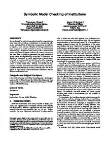
Formula 7 is a special case of the formula ωǫ given by ωǫ = ∃ǫ.ǫ ≥ x0 ∧ φ + ǫ for some SL formula φ. From a geometric viewpoint, φ is a region in Rn and ωǫ is the shadow of φ for a light source at ∞n . Examples of φ and the corresponding ωǫ are shown in Figures 1(a) and 1(c) respectively. We can transform ωǫ to an equivalent SL formula φub by eliminating upper bounds on x0 , i.e., Boolean variables of the form e⊲⊳,c i,0 . The transformation is performed iteratively in the following steps:

m ,cm 2 ,c2 1 ,c1 be Boolean literals encoding all , . . . , e⊲⊳ , ei⊲⊳2 ,0 1. Let φ0 = φ. Let ei⊲⊳1 ,0 im ,0 upper bounds on x0 that occur in φ. 2. For j = 1, 2, . . . , m, we construct φj as follows: ⊲⊳j ,cj to get (a) Replace all occurrences of xij ⊲⊳j x0 + cj in φj−1 with eij ,0

φ0,j−1 bool . 6 (b) Construct φ0,j−1 cons , the conjunction of all transitivity constraints for x0 ⊲⊳j ,cj 0,j−1 involving eij ,0 and clock variables in φbool . (c) Construct the formula φj , a disjunction of two terms: 0,j−1 0,j−1 ⊲⊳ ,c ⊲⊳ ,c φj = {(φ0,j−1 bool ∧φcons )|e j j =true } ∨ {[¬(xij ⊲⊳j x0 +cj )]∧[φbool |e j j =false ]} ij ,0

ij ,0

The first disjunct is the region obtained by dropping the bound xij ⊲⊳j x0 + cj from convex sub-regions of φj−1 where it is a lower bound on xij , while letting time elapse backward. The second disjunct corresponds to sub-regions where ¬(xij ⊲⊳j x0 + cj ) is an upper bound; these regions are left unchanged. The output of the above transformation, φub , is given by φub = φm . The correctness of this procedure is formalized in the following theorem. Theorem 2. ωǫ and φub are equivalent. Example 2. Let the subformula φ of ωǫ be φ = (x1 ≥ x0 + 3 ∧ x2 ≤ x0 + 2) ∨ (x1 < x0 + 3 ∧ x2 ≥ x0 + 3) φ is depicted geometrically as the shaded region in Figure 1(a). It comprises two

x2

x2

3

3

2-

2x1

3 (a) φ0 = φ

3 x1 = x2 + 1 (b) φ1

x2

3 2x1

x1 = x2

3

x1

(c) φ2 = ωǫ

Fig. 1. Eliminating upper bounds on x0 . Only the positive quadrant is shown.

sub-regions, one for each disjunct. The lower bounds on these regions, x1 ≥ x0 +3 ≥,3 and x2 ≥ x0 + 3, are upper bounds on x0 . We encode these by e≥,3 1,0 and e2,0 . Figure 1(b) shows φ1 , the result of eliminating e≥,3 1,0 . Formally, we calculate ≥,3 ≥,3 φ0,0 bool = (e1,0 ∧ x2 ≤ x0 + 2) ∨ (¬e1,0 ∧ x2 ≥ x0 + 3) ≥,3 φ0,0 cons = (e1,0 ∧ x2 ≤ x0 + 2) =⇒ (x1 ≥ x2 + 1) 6

We can use the optimization technique of Section 4.1 in this step.

Then, applying step 2(c) of the transformation, we get φ1 = (x2 ≤ x0 + 2 ∧ x1 ≥ x2 + 1) ∨ (x1 < x0 + 3 ∧ x2 ≥ x0 + 3) Similarly, in the next iteration, we introduce and eliminate e≥,3 2,0 to get φ2 , shown in Figure 1(c), which is equivalent to ωǫ . ⊓ ⊔ Note that the QSL formula obtained after eliminating the inner quantifier in Formula 4 is not of the form ωǫ , and so we cannot avoid introducing the δ variable. 4.3

Eliminating Infeasible Paths in BDDs

Suppose β is the Boolean encoding of SL formula φ. Let φcons denote the conjunction of transitivity constraints for all real-valued variables in φ, and let βcons denote its Boolean encoding. Finally, denote the BDD representations of β and βcons by Bdd(β) and Bdd(βcons ) respectively. We would like to eliminate paths in Bdd(β) that violate transitivity constraints, i.e., those corresponding to assignments to variables in β for which βcons = false. We can do this by using the BDD Restrict operator, replacing Bdd(β) by Restrict(Bdd(β), Bdd(βcons )). Informally, Restrict(Bdd(β), Bdd(βcons )) traverses Bdd(β), eliminating a path on which βcons is false as long as it doesn’t involve adding new nodes to the resulting BDD. Details about the Restrict operator may be found in the paper by Coudert and Madre [7]. Since eliminating infeasible paths in a large BDD can be quite time consuming, we only apply this optimization to the BDD for the set of reachable states, once on each fixpoint iteration.

5

Experimental Results

We implemented a BDD-based model checker called TMV, that is written in OCaml and uses the CUDD package7 . We have performed preliminary experiments comparing the performance of our model checker for both reachability and non-reachability TCTL properties. For reachability properties, we compare against the other unbounded, fully symbolic model checkers, viz., a DDD-based checker (DDD) [12] and Red version 4.1 [17], which have been shown to outperform Uppaal2k and Kronos for reachability analysis. For non-reachability properties, such as checking that a system is non-zeno, we compare against Kronos and Red, the only other unbounded model checkers that check such properties. We ran two experiments using Fischer’s time-based mutual exclusion protocol. The first experiment compared our model checker against DDD and Red, checking that the system preserves mutual exclusion (a reachability property). In the second, we compared against Kronos and Red for checking that the 7

http://vlsi.colorado.edu/~fabio/CUDD

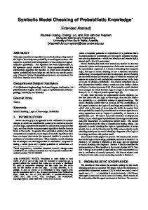
product automaton is non-zeno (a non-reachability property). All experiments were run on a notebook computer with a 1 GHz Pentium-III processor and 128 MB RAM, running Linux. We ran DDD, Kronos, and Red with their default options. TMV used a static BDD variable ordering that is the same as the one used for the corresponding Boolean variables and separation predicates in DDD and is described in detail in our technical report [14]. Table 1(a) shows the results of the comparison against DDD and Red for checking mutual exclusion for increasing numbers of processes. For DDD and TMV, the table lists both the run-times and the peak number of nodes in the decision diagram for the reachable state set. We find that DDD outperforms TMV due to the blow-up of BDDs. In spite of the optimizations of Section 4, the peak node count in the case of DDD is less than that for TMV, since the local reduction operations performed by DDD during node creation can eliminate unnecessary DDD nodes without adding any time overhead. For example, DDD can reduce a function of the form e1 ∧ e2 ∧ e3 under the transitivity constraint [e1 ∧ e2 ] =⇒ e3 to simply the conjunction e1 ∧ e2 . The BDD Restrict operator cannot always achieve this as it is sensitive to the BDD variable ordering. Furthermore, TMV contains many other BDDs, such as those for the transitivity constraints, to which we do not apply the Restrict optimization due to its runtime overhead. Finally, in comparison to Red, we see that while TMV is faster on the smaller benchmarks, Red’s superior memory performance enables it to complete for 7 processes while TMV runs out of memory. Num. Red DDD TMV Proc. Time Time Reach Set Time Reach Set (sec.) (sec.) (peak (sec.) (peak nodes) nodes) 3 0.21 0.06 130 0.11 101 4 1.13 0.14 352 0.38 316 5 4.53 0.33 854 1.85 1127 6 15.11 0.90 2375 17.41 4685 7 46.31 2.65 6346 * *

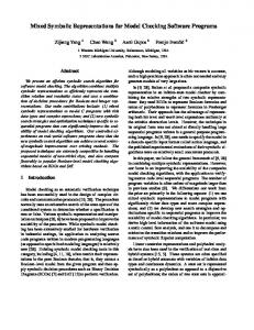
Num. Kronos Red TMV Proc. Time Time Time Reach Set (sec.) (sec.) (sec.) (peak nodes) 3 0.03 0.28 0.24 28 4 0.23 1.30 0.44 39 5 1.98 5.05 0.80 54 6 * 17.80 2.15 69 7 * 57.95 6.61 88

(a) Mutual Exclusion

(b) Non-Zenoness

Table 1. Checking properties of Fischer’s protocol for increasing numbers of processes. A “*” indicates that the model checker ran out of memory.

Table 1(b) shows the comparison with Kronos and Red for checking nonzenoness. The time for Kronos is the sum of the times for product construction and backward model checking. We notice that while Kronos does better for smaller numbers of processes, the product automaton it constructs grows very quickly, becoming too large to construct at 6 processes. The run times for TMV, on the other hand, grow much more gradually, demonstrating the advantages of a fully symbolic approach. For this property, the BDDs remain small even for larger numbers of processes. Thus, TMV outperforms Red, especially as the number of processes increases. These results indicate that when the representation (BDDs) remains small, Boolean methods for quantifier elimination and deciding SL can outperform non-Boolean methods by a significant factor.

Although they are preliminary, our results indicate that our model checker based on a general purpose BDD package can outperform methods based on specialized representations of SL formulas. We are working on improving our current methods of eliminating unnecessary BDD nodes, and are also starting to work on a SAT-based implementation. Acknowledgments. We thank Jo¨el Ouaknine, Ofer Strichman, and the reviewers for useful comments. We also thank the authors of DDD and Red for providing their tools and answering our queries. This research was supported in part by a NDSEG Fellowship and by ARO grant DAAD19-01-1-0485.

References 1. L. Aceto, P. Bouyer, A. Burgueno, and K. G. Larsen. The power of reachability testing for timed automata. Theoretical Computer Science, 300(1-3):411-475, 2003. 2. R. Alur. Timed automata. In Proc. CAV’99, LNCS 1633, pages 8–22. 3. G. Audemard, A. Cimatti, A. Korniowicz, and R. Sebastiani. Bounded model checking for timed systems. In Proc. FORTE’02, LNCS 2529, pages 243–259. 4. G. Behrmann, K. G. Larsen, J. Pearson, C. Weise, and W. Yi. Efficient timed reachability analysis using clock difference diagrams. In Proc. CAV’99, LNCS 1633, 341–353. 5. D. Beyer. Improvements in BDD-based reachability analysis of timed automata. In Proc. FME’01, LNCS 2021, pages 318–343. 6. M. Bozga, O. Maler, A. Pnueli, and S. Yovine. Some progress in the symbolic verification of timed automata. In Proc. CAV’97, LNCS 1254, pages 179–190. 7. O. Coudert and J. C. Madre. A unified framework for the formal verification of sequential circuits. In Proc. ICCAD’90, pages 126–129. 8. G. B. Dantzig and B. C. Eaves. Fourier-Motzkin elimination and its dual. Journal of Combinatorial Theory A, 14:288–297, 1973. 9. T. A. Henzinger, X. Nicollin, J. Sifakis, and S. Yovine. Symbolic model checking for real-time systems. Information and Computation, 111(2):193–244, 1994. 10. M. Koubarakis. Complexity results for first-order theories of temporal constraints. In Proc. KR’94, pages 379–390. 11. K. L. McMillan. Applying SAT methods in unbounded symbolic model checking. In Proc. CAV’02, LNCS 2404, pages 250–264. 12. J. B. Møller. Simplifying fixpoint computations in verification of real-time systems. In Proc. RTTOOLS’02 workshop. 13. P. Niebert, M. Mahfoudh, E. Asarin, M. Bozga, N. Jain, and O. Maler. Verification of timed automata via satisfiability checking. In Proc. FTRTFT’02, LNCS 2469. 14. S. A. Seshia and R. E. Bryant. A Boolean approach to unbounded, fully symbolic model checking of timed automata. Technical Report CMU-CS-03-117, Carnegie Mellon University, 2003. 15. O. Strichman. Optimizations in decision procedures for propositional linear inequalities. Technical Report CMU-CS-02-133, Carnegie Mellon University, 2002. 16. O. Strichman, S. A. Seshia, and R. E. Bryant. Deciding separation formulas with SAT. In Proc. CAV’02, LNCS 2404, pages 209–222. 17. F. Wang. Efficient verification of timed automata with BDD-like data-structures. In Proc. VMCAI’03, LNCS 2575, pages 189–205. 18. S. Yovine. Kronos: A verification tool for real-time systems. Software Tools for Technology Transfer, 1(1/2):123–133, Oct. 1997.