Hindawi Publishing Corporation Mathematical Problems in Engineering Volume 2014, Article ID 187275, 11 pages http://dx.doi.org/10.1155/2014/187275
Research Article Uncertain Programming for Network Revenue Management Deyi Mou and Xiaoxin Wang Institute of Mathematics for Applications, Civil Aviation University of China, Tianjin 300300, China Correspondence should be addressed to Xiaoxin Wang;
[email protected] Received 18 March 2014; Revised 14 May 2014; Accepted 19 May 2014; Published 9 June 2014 Academic Editor: Andy H. F. Chow Copyright © 2014 D. Mou and X. Wang. This is an open access article distributed under the Creative Commons Attribution License, which permits unrestricted use, distribution, and reproduction in any medium, provided the original work is properly cited. The mathematical model for airline network seat inventory control problem is usually investigated to maximize the total revenue under some constraints such as capacities and demands. This paper presents a chance-constrained programming model based on the uncertainty theory for network revenue management, in which the fares and the demands are both uncertain variables rather than random variables. The uncertain programming model can be transformed into a deterministic form by taking expected value on objective function and confidence level on the constraint functions. Based on the strategy of nested booking limits, a solution method of booking control is developed to solve the problem. Finally, this paper gives a numerical example to show that the method is practical and efficient.
1. Introduction After the deregulations in the airline industry, the revenue management techniques have become indispensable for airline seat inventory control. A central problem in airline revenue management is determining optimal decision rules for sequentially accepting or denying itinerary requests. So it is necessary to develop mathematical models to determine complex booking control strategies. The optimization methods on seat inventory control problem with multiple-fare classes can be separated into the single-leg optimization method and the network optimization method. Based on the optimized frequency, each optimization method can be sorted out the static method and the dynamic method. In brief, the dynamic nature of the arrivals of the requests over time is not explicitly considered in the static method, whereas the mutability in the demand is taken into account in the dynamic method as the end of the reservation period approaches and the seat capacity diminishes. The single-leg optimization method firstly appeared in the research of Littlewood [1]. He studied a seat inventory control problem with two-fare classes on a single leg and proposed a marginal seat revenue rule applied into a twoprice, single-leg model. Belobaba [2, 3] extended this idea to a multiclass problem and introduced the expected marginal
seat revenue heuristic for the general approach. Wollmer [4], Brumelle and McGill [5], and Robinson [6] further studied the single-leg problem with multiple-fare classes. They developed algorithms to find the optimal booking control policy under the assumption that the probability distributions of the demands for different fare classes were known. Lee and Hersh [7] developed a discrete-time dynamic programming model to find an optimal booking control policy without requiring any assumptions about the arrival mode for the manifold booking classes. Liang [8] proposed a continuous-time, stochastic, dynamic programming model and showed that a threshold control policy was optimal. Feng and Xiao [9] presented a stochastic control model to dynamically tackle with seat inventory control problem. For the network optimization method, Glover et al. [10] initially described a minimum cost network flow formulation with deterministic demand without focusing on the stochastic elements. After that, a solution method for the sequential allocation of seats under the assumption of stochastic demand was provided by Wang [11]. Wollmer [12] proposed a linear programming model that considered stochastic demand. Dror et al. [13] proposed a similar deterministic network minimum cost flow formulation that allowed for cancellations as deterministic losses on arcs in the network. Curry [14] developed a combined mathematical model for a multiclass seat inventory control problem. Williamson
2 [15] studied two network-based mathematical programming models. The first model incorporated probabilistic demand and the second model simplified the problem by substituting stochastic demand by its expectation. Wong et al. [16] applied nesting techniques into a multiclass seat inventory control problem. de Boer et al. [17] proposed stochastic linear programming for network revenue management and developed the nesting technique of Williamsion. Bertsimas and De Boer [18] and van Ryzin and Vulcano [19] used simulation-based optimization methods that also investigated nesting over the network. Cooper and Homem-De-Mello [20] proposed a decomposition method combining mathematical programming methods and Markov decision process. Recently, ˙Ilker Birbil et al. [21] proposed a framework for solving airline revenue management problems on large networks. With the fast development of civil aviation industry, many airlines often create new routes. Due to lacking reliable data and accurate information, the methods in the literature above become invalid for these new routes. On the other hand, when unconventional sudden events such as war, atrocious weather, and earthquake, happen, the cumulative data of computer reservation system is no longer trustworthy. There are some limitations when the traditional stochastic models above deal with such problems at this situation. In the two cases, we have to invite some experts to evaluate their degree of belief that each event will occur. However, humans tend to overweigh unlikely events (Kahnema and Tversky [22]); thus, the degree of belief may have a much larger range than the real frequency. In this situation, if we insist on dealing with the degree of belief using the probability theory, some counterintuitive results will be obtained (Liu [23]). In revenue management of the above two cases, as we stated before, the domain experts invited are likely to overrate the market demand on the new routes and underestimate the market demand under the circumstances of unconventional sudden events. If the belief degree of the market demand is treated as probability, we have no choice but to increase the capacity on the new routes and reduce the capacity under the circumstances of unconventional sudden events. This will cause great losses in revenue for airlines. This conclusion seems unacceptable and then the belief degree cannot be treated as probability. In order to deal with the experts’ degree of belief, the uncertainty theory was founded by Liu [24] and refined by Liu [25] in 2013. Many researchers have contributed to this area. The uncertainty theory has been applied to uncertain programming, uncertain risk analysis, uncertain game, uncertain inference, uncertain logic, uncertain finance, and uncertain optimal control (Liu [25]). Nowadays, the uncertainty theory has become a branch of axiomatic mathematics to model human uncertainty (Liu [26]). Depending on the analysis as mentioned above, we think that it is necessary to apply the uncertainty theory as a basic approach to model the uncertainty in the revenue management of the two cases above. In this paper, we propose the chance-constrained programming model based on the uncertainty theory to deal with the uncertain factors. The rest of this paper is structured as follows. In Section 2, some basic concepts and properties in uncertainty theory
Mathematical Problems in Engineering used throughout this paper are introduced. In Section 3, an uncertain programming model is constructed. According to inverse uncertainty distribution, the model can be transformed to its deterministic form. In Section 4, we present a solution method of booking control on the basis of the strategy of nested booking limits. After that, a numerical example is given in Section 5. At last, a brief summary is presented in Section 6.
2. Preliminaries In this section, some basic definitions and arithmetic operations of uncertainty theory needed throughout this paper are presented. Definition 1 (Liu [24]). Let Γ be a nonempty set and L a 𝜎algebra over Γ. Each element Λ ∈ L is called an event. The set function M is called an uncertain measure if it satisfies the following four axioms: Axiom 1 (Normality). M{Γ} = 1; Axiom 2 (Monotonicity). M{Λ 1 } ≤ M{Λ 2 } whenever Λ 1 ⊂ Λ 2; Axiom 3 (Self-Duality). M{Λ} + M{Λ 𝑐 } = 1 for any event Λ; Axiom 4 (Countable Subadditivity). For every countable sequence of events {Λ 𝑖 }, we have { {∞ } } ∞ M {⋃Λ 𝑖 } ≤ ∑M {Λ 𝑖 } . (1) { 𝑖=1 } 𝑖=1 { } Definition 2 (Liu [24]). Let Γ be a nonempty set, L a 𝜎algebra over Γ, and M an uncertain measure. Then the triple (Γ, L, M) is called on uncertainty space. Definition 3 (Liu [24]). An uncertain variable 𝜉 is a measurable function from an uncertainty space (Γ, L, M) to the set of real numbers; that is, for any Borel set 𝐵 of real numbers, the set {𝜉 ∈ 𝐵} = {𝛾 ∈ Γ | 𝜉 (𝛾) ∈ 𝐵}
(2)
is an event. For a sequence of uncertainty variables 𝜉1 , 𝜉2 , . . . , 𝜉𝑛 and a measurable function 𝑓, Liu [24] proved that 𝜉 = 𝑓(𝜉1 , 𝜉2 , . . . , 𝜉𝑛 ) defined as 𝜉(𝛾) = 𝑓(𝜉1 (𝛾), 𝜉2 (𝛾), . . . , 𝜉𝑛 (𝛾)), ∀𝛾 ∈ Γ is also an uncertain variable. In order to describe an uncertain variable, a concept of uncertainty distribution is introduced as follows. Definition 4 (Liu [24]). The uncertainty distribution Φ of an uncertain variable 𝜉 is defined by Φ (𝑥) = M {𝜉 ≤ 𝑥} ,
(3)
for any real number 𝑥. Peng and Iwamura [27] proved that a function Φ: 𝑅 → [0, 1] is an uncertainty distribution if and only if it is
Mathematical Problems in Engineering
3
a monotone increasing function except for Φ(𝑥) ≡ 0 or Φ(𝑥) ≡ 1. The inverse function Φ−1 is called the inverse uncertainty distribution of 𝜉. Inverse uncertainty distribution is an important tool in the operation of uncertain variables. Theorem 5 (Liu [24]). Let 𝜉1 , 𝜉2 , . . . , 𝜉𝑛 be independent uncertain variables with regular uncertainty distributions Φ1 , Φ2 , . . . , Φ𝑛 , respectively. If 𝑓(𝑥1 , 𝑥2 , . . . , 𝑥𝑛 ) is strictly increasing with respect to 𝑥1 , 𝑥2 , . . . , 𝑥𝑚 and strictly decreasing with respect to 𝑥𝑚+1 , 𝑥𝑚+2 , . . . , 𝑥𝑛 , then 𝜉 = 𝑓 (𝜉1 , 𝜉2 , . . . , 𝜉𝑛 )
(4)
is an uncertain variable with inverse uncertainty distribution −1 −1 Ψ−1 (𝛼) = 𝑓 (Φ−1 1 (𝛼) , . . . , Φ𝑚 (𝛼) , Φ𝑚+1 (1 − 𝛼) , . . . ,
Φ−1 𝑛 (1 − 𝛼)) .
(5)
Expected value is the average of an uncertain variable in the sense of uncertain measure. It is an important index to rank uncertain variables. Definition 6 (Liu [24]). Let 𝜉 be an uncertain variable. Then the expected value of 𝜉 is defined by ∞
0
0
−∞
𝐸 [𝜉] = ∫ M {𝜉 ≥ 𝑟} 𝑑𝑟 − ∫
M {𝜉 ≤ 𝑟} 𝑑𝑟,
In order to calculate the expected value via inverse uncertainty distribution, Liu and Ha [28] proved that 1
0
Φ−1 𝑛
(7)
𝑥ODF : the number of seats reserved for each separate ODF; 𝑁 : the total number of flight legs in the ODF network; 𝑆𝑙 : the set of ODF combinations available on flight leg; 𝐶𝑙 : the seat capacity on leg 𝑙; 𝑓ODF : the fare required for an ODF. In order to facilitate the analysis, we make some reasonable assumptions as follows. (a) The flight market demand exceeds its capacity supply. (b) Overbooking is not considered by the model discussed here. Next, based on the analysis of the decision making process, the general problem is formulated as follows [15]:
(1 − 𝛼) 𝑑𝛼
under the condition described in Theorem 5. Generally, the expected value operator 𝐸 has no linearity property for arbitrary uncertain variables. But, for independent uncertain variables 𝜉 and 𝜂 with finite expected values, we have 𝐸 [𝑎𝜉 + 𝑏𝜂] = 𝑎𝐸 [𝜉] + 𝑏𝐸 [𝜂] ,
3.2. Model Development. At first, we introduce the following notations to represent the mathematical formulation throughout the remainder of this paper:
𝐷ODF : the deterministic aggregated demand for each ODF; (6)
provided that at least one of the two integrals is finite.
−1 −1 𝐸 [𝜉] = ∫ 𝑓 (Φ−1 1 (𝛼)) , . . . , Φ𝑚 (𝛼) , Φ𝑚+1 (1 − 𝛼) , . . . ,
ODF combinations. Each ODF in the network is constitutive of one or more flight legs. The limited capacity on each flight leg has to be made full use of in the most profitable way. This can be achieved by limiting the number of seats available to the less lucrative classes. So the problem is to allocate all seats of each flight leg to the related ODF in the most profitable way. Due to its economic importance in the airline, the problem has been extensively studied. In this paper, the network seat inventory control problem will be modeled by the chance-constrained programming based on the uncertainty theory in which the fare and the demand of each ODF are assumed to be uncertain variables with given uncertainty distributions.
(8)
for any real numbers 𝑎 and 𝑏.
3. Uncertain Programming Model for Multiple-Leg Network Seat Inventory Control 3.1. Problem Description. Because an airline wants to maximize revenue from the whole network, the researchers on this field focus on the network-based models now. Airlines usually provide thousands of such combinations of origin, destination and fare class (ODF). Therefore determining a comprehensive booking control strategy for the entire network is crucially important. The objective of network seat inventory control is to maximize the airline’s expected revenue from its supply of
max
∑ 𝑓ODF 𝑥ODF ODF
s.t. ∑ 𝑥ODF ≤ 𝐶𝑙
∀flight legs 𝑙 = 1, . . . , 𝑁,
(9)
ODF∈𝑆𝑙
𝑥ODF ≤ 𝐷ODF
∀ODF,
𝑥ODF ≥ 0 integer
∀ODF.
In the above model, the quantities 𝑓ODF and 𝐷ODF are all assumed to be crisp numbers. However, when there are new routes created by the airlines or the emergency takes place sometimes, the quantities generally are not fixed but obtained from experience evaluation or expert knowledge. In this case, we may assume the quantities are uncertain variables. Then the model (9) is only a conceptual model rather than a mathematical model because there does not exist a natural ordership in an uncertain world. Here we take expected value criterion on the objective function and
4
Mathematical Problems in Engineering
confidence level on the constraint functions (Liu [25]). Then the model (9) turns into the following mathematical model: max
Theorem 9. Assume that 𝑓ODF and 𝐷ODF are independent uncertain variables with uncertainty distributions 𝜙ODF and 𝜓ODF . Then the model (10) is equivalent to the following model: 1
𝐸 [ ∑ 𝑓ODF 𝑥ODF ]
−1 ∑ 𝑥ODF ∫ 𝜙ODF (𝛼) 𝑑𝛼
max
ODF
ODF
s.t.
0
s.t. ∑ 𝑥ODF ≤ 𝐶𝑙
∀flight legs 𝑙 = 1, . . . , 𝑁,
(10)
∑ 𝑥ODF ≤ 𝐶𝑙
ODF∈𝑆𝑙
𝑀 {𝑥ODF ≤ 𝐷ODF } ≥ 𝛽ODF 𝑥ODF ≥ 0 integer
−1 𝑥ODF ≤ 𝜓ODF (1 − 𝛽ODF )
∀ODF,
Corollary 7. Assume the objective function 𝑓(𝑥, 𝜉1 , 𝜉2 , . . . , 𝜉𝑛 ) is strictly increasing with respect to 𝜉1 , 𝜉2 , . . . , 𝜉𝑚 and strictly decreasing with respect to 𝜉𝑚+1 , 𝜉𝑚+2 , . . . , 𝜉𝑛 . If 𝜉1 , 𝜉2 , . . . , 𝜉𝑛 are independent uncertain variables with uncertainty distributions Φ1 , Φ2 , . . . , Φ𝑛 , respectively, then the expected objective function 𝐸[𝑓(𝑥, 𝜉1 , 𝜉2 , . . . , 𝜉𝑛 )] is equal to
0
(12)
Φ−1 𝑛 (1 − 𝛼)) ≤ 0.
1
𝐸 [ ∑ 𝑓ODF 𝑥ODF ] = ∑ 𝑥ODF ∫ 𝜙−1 ODF (𝛼) 𝑑𝛼. ODF
0
ODF
(15)
Since that 𝑀 {𝑥ODF ≤ 𝐷ODF } ≥ 𝛽ODF
(16)
𝑀 {−𝐷ODF + 𝑥ODF ≤ 0} ≥ 𝛽ODF
(17)
is equivalent to
and the function −𝐷ODF + 𝑥ODF is strictly decreasing with respect to 𝐷ODF with uncertainty distribution 𝜓ODF , it follows from Corollary 8 that we have −1 −𝜓ODF (1 − 𝛽ODF ) + 𝑥ODF ≤ 0,
(18)
−1 𝑥ODF ≤ 𝜓ODF (1 − 𝛽ODF ) .
(19)
that is,
The theorem is thus verified.
4. Solution Method of Booking Control 4.1. The Strategy of Nested Booking Limits. In the model (14), 1 −1 we use 𝑓ODF to denote ∫0 𝜙ODF (𝛼)𝑑𝛼 and 𝐷ODF to denote −1 𝜓ODF (1 − 𝛽ODF ). Then the relaxation of the model (14) is max
holds if and only if −1 −1 𝑔 (𝑥, Φ−1 1 (𝛼) , . . . , Φ𝑘 (𝛼) , Φ𝑘+1 (1 − 𝛼) , . . . ,
Proof. The function ∑ODF 𝑓ODF 𝑥ODF is strictly increasing with respect to 𝑓ODF and 𝑓ODF are independent uncertain variables with uncertainty distributions 𝜙ODF , respectively. By using Corollary 7, we obtain
(11)
Corollary 8. Assume the constraint function 𝑔(𝑥, 𝜉1 , 𝜉2 , . . . , 𝜉𝑛 ) is strictly increasing with respect to 𝜉1 , 𝜉2 , . . . , 𝜉𝑘 and strictly decreasing with respect to 𝜉𝑘+1 , 𝜉𝑚𝑘2 , . . . , 𝜉𝑛 . If 𝜉1 , 𝜉2 , . . . , 𝜉𝑛 are independent uncertain variables with uncertainty distributions Φ1 , Φ2 , . . . , Φ𝑛 , respectively, then the chance constrain M {𝑔 (𝑥, 𝜉1 , 𝜉2 , . . . , 𝜉𝑛 ) ≤ 0} ≥ 𝛼
∀ODF,
𝑥ODF ≥ 0 integer ∀ODF.
where 𝛽ODF are some predetermined confidence levels for all ODF. In practical applications, the uncertainty distributions of uncertain variables 𝑓ODF and 𝐷ODF and the confidence levels 𝛽ODF are determined by linear interpolation method, the principle of least squares, the method of moments, and the Delphi method from expert’s experimental data (Liu [25]). How do we obtain expert’s experimental data? Liu [25] proposed a questionnaire survey for collecting expert’s experimental data. In this paper, we assume that the uncertainty distributions of uncertain variables 𝑓ODF and 𝐷ODF and the confidence levels 𝛽ODF have been determined. In order to solve model (10), firstly, we introduce two corollaries which were from the uncertainty theory (Liu [25]).
−1 −1 −1 ∫ 𝑓 (𝑥, Φ−1 1 , . . . , Φ𝑚 , Φ𝑚+1 , . . . , Φ𝑛 ) 𝑑𝛼.
(14)
ODF∈𝑆𝑙
∀ODF,
1
∀flight legs 𝑙 = 1, . . . , 𝑁,
∑ 𝑓ODF 𝑥ODF ODF
s.t. (13)
Secondly, the next theorem shows that the model (10) is equivalent to a deterministic model, for which many efficient algorithms have been designed.
∑ 𝑥ODF ≤ 𝐶𝑙
∀flight legs 𝑙 = 1, . . . , 𝑁,
ODF∈𝑆𝑙
𝑥ODF ≤ 𝐷ODF
∀ODF,
𝑥ODF ≥ 0 ∀ODF.
(20)
Mathematical Problems in Engineering
5 Table 1: Simulated reservation data.
ODF ABY ABT BCY BCT ACY ACT
t = 10 3 13 0 15 2 10
t=9 3 5 2 5 0 2
t=8 3 8 1 11 0 5
t=7 5 7 5 9 1 6
t=6 4 1 4 9 2 2
Table 2: Parameters of normal distribution of demand. 1 (42, 2)
𝑁(𝑒𝑖 , 𝜎𝑖 )
2 (66, 2)
3 (41, 3)
4 (71, 4)
5 (35, 1)
6 (50, 3)
The whole booking time should be partitioned into a few time periods of reservation; for example, a day is a time period of reservation. In order to facilitate the analysis, we describe the model (20) in the form of the matrix and the vector considering the time period of reservation. For this, we introduce the following notations: 𝐼: the total number of flight legs in the ODF network; 𝑖: index for set of flight legs; 𝐽: the total number of the ODF; 𝑗: index for set of the ODF; 𝑡: index for the time period of reservation; 𝑇
𝐶𝑡 = [𝐶1𝑡 , 𝐶2𝑡 , . . . , 𝐶𝑖𝑡 , . . . , 𝐶𝐼𝑡 ] : the seat capacity on each flight leg in the reservation time period 𝑡; 𝐹𝑡
=
𝑡
𝑡
𝑡
𝑡 𝑇
[𝑓1 , 𝑓2 , . . . , 𝑓𝑗 , . . . 𝑓𝐽 ] : the corresponding
𝑓ODF for each separate ODF in the reservation time period 𝑡; 𝑡
𝑡 𝑡 𝑡 𝑡 𝑇 [𝐷1 , 𝐷2 , . . . , 𝐷𝑗 , . . . , 𝐷𝐽 ] :
the corresponding 𝐷 = 𝐷ODF for each separate ODF in the reservation time period 𝑡; 𝑇
𝑋𝑡 = [𝑥1𝑡 , 𝑥2𝑡 , . . . , 𝑥𝑗𝑡 , . . . , 𝑥𝐽𝑡 ] : the number of seats reserved for each separate ODF in the reservation time period 𝑡; 𝐴 = (𝑎𝑖𝑗 )𝐼×𝐽 : the matrix denotation of flight legs that each ODF travels, where if the ODF 𝑗 travels the flight leg 𝑖, then 𝑎𝑖𝑗 = 1, otherwise 𝑎𝑖𝑗 = 0; 𝐴𝑗 : the 𝑗th column of the matrix 𝐴, denoting the flight legs that the ODF 𝑗 travels. The model (20) is described as follows in the form of the matrix and the vector: LP (𝐶𝑡 , 𝐷𝑡 ) = max
𝑇
(𝐹𝑡 ) 𝑋𝑡
s.t. 𝑡
𝑡
𝐴𝑋 ≤ 𝐶 , 0 ≤ 𝑋 𝑡 ≤ 𝐷𝑡 .
t=5 1 2 8 8 9 4
t=4 3 6 6 2 1 7
t=3 7 2 4 3 7 4
t=2 8 5 7 4 5 3
t=0 8 2 4 0 5 1
The dual problem of the model above can be described as follows: DLP (𝐶𝑡 , 𝐷𝑡 ) = min
𝑇
𝑇
[(𝑃𝑡 ) 𝐶𝑡 + (𝑄𝑡 ) 𝐷𝑡 ]
s.t. 𝐴𝑇 𝑃𝑡 + 𝑄𝑡 ≥ 𝐹𝑡 ,
(22)
𝑃𝑡 , 𝑄𝑡 ≥ 0, 𝑇
where 𝑃𝑡 = [𝑃1𝑡 , 𝑃2𝑡 , . . . , 𝑃𝑖𝑡 , . . . , 𝑃𝐼𝑡 ] denotes the shadow prices corresponding to each flight leg and 𝑄𝑡 = [𝑄1𝑡 , 𝑄2𝑡 , . . . , 𝑄𝑗𝑡 , . . . , 𝑄𝐽𝑡 ]𝑇 denotes the shadow prices corresponding to each 𝐷ODF . Bid price control method is one of the prevalent methods of network seat inventory control. The bid price of each ODF is equal to the sum of shadow prices of the flight legs that the ODF crosses. A booking request for a passenger from the ODF is rejected if the bid price of the ODF exceeds the fare for the ODF and is accepted otherwise. Although bid price control method has been used in the actual operations of the airlines, it has a few shortcomings as follows. (a) Each ODF’s contribution to network revenue is not considered in the bid price control method. (b) When calculating shadow prices using the relevant models, the solution of the model may be degenerate solution. This will cause the multiple bid prices of an ODF. (c) The fares of most of the passengers on the flight just exceed the bid prices so that airlines suffer losses. For this, we present a nesting control method based on the network contribution value for the above uncertain programming model. First, we define an ODF’s net contribution value to network revenue in the reservation time period 𝑡 as the expected fare for the ODF in the reservation time period 𝑡 minus the opportunity cost of the ODF in the reservation time period 𝑡, that is, 𝑡
NCV𝑡𝑗 = 𝑓𝑗 − OC𝑡𝑗 , (21)
t=1 11 5 7 2 3 1
(23)
where NCV𝑡𝑗 denotes the net contribution value of the ODF 𝑗 to network revenue in the reservation time period 𝑡 and OC𝑡𝑗 denotes the opportunity cost of the ODF 𝑗 in the reservation time period 𝑡.
6
Mathematical Problems in Engineering Table 3: Parameters of normal distribution of fare. 1 (1000, 80)
𝑁(𝑒𝑖 , 𝜎𝑖 )
2 (800, 40)
3 (400, 20)
4 (320, 10)
5 (1200, 90)
6 (960, 50)
Table 4: The seat inventory control for t = 10.
t = 10
𝑗
ODF
𝑓𝑗𝑡
NCV𝑡𝑗
𝑥𝑗𝑡
BL𝑡
Simulated reservation data
The number of accepted seats
ABY ABT BCY BCT ACY ACT
1000 800 400 320 1200 960
200 0 80 0 80 −160
42 63 41 64 35 10
140 63 105 64 98 0
3 13 0 15 2 10
3 13 0 15 2 0
Table 5: The seat inventory control result. The combination of the ODF
The total number of accepted seats
ABY ABT BCY BCT ACY ACT
52 54 48 58 30 4
The total expected revenue
𝑡
𝑓𝑗 − [LP(𝐶𝑡 , 𝐷𝑡 ) − LP(𝐶𝑡 − 𝐴𝑗 , 𝐷𝑡 )]. Otherwise, NCV𝑡𝑗 = −∞ where ∞ denotes a large enough number. Finally, we rank the ODF on the basis of their net contribution value to network revenue to determine the nesting level. If some of the ODFs have the same net contribution value to network revenue, we can rank the ODF on the basis of their expected fare.
172800
Table 6: The seat inventory control result of the bid price control method. The combination of the ODF
The total number of accepted seats
ABY ABT BCY BCT ACY ACT
48 54 45 57 30 8
The total expected revenue
net contribution values of the ODF to network revenue. In this case, we will use the following method to calculate the net contribution value of the ODF to network revenue in the reservation time period 𝑡. If 𝐶𝑡 − 𝐴𝑗 ≥ 0, then NCV𝑡𝑗 =
4.2. The Algorithm for Nested ODF-Based Booking Control. Every time a booking request arrives for any ODF in the network, a quick decision should be made whether or not to accept the request. We have to specify a booking control strategy for the decision. We propose the algorithm for nested ODF-based booking control. The notations used in the following algorithm are given as below: 𝑇
𝑗
𝑋𝑡 = [𝑥𝑡1 , 𝑥𝑡2 , . . . , 𝑥𝑡 , . . . , 𝑥𝑡𝐽 ] : the number of seats reserved for each separate ODF in the reservation time period 𝑡 after ranking the elements of 𝑋𝑡 according to the nesting level;
171120
𝑗
𝑁(𝑒𝑖 , 𝜎𝑖 )
1 (40, 2)
2 (56, 2)
3 (39, 3)
4 (61, 4)
5 (34, 1)
6 (42, 3)
The opportunity cost OC𝑡𝑗 of the ODF 𝑗 in the reservation time period 𝑡 is calculated based on the DLP model as follows: OC𝑡𝑗
𝑡 𝑇
𝑗
= (𝑃 ) 𝐴
𝑇
PL𝑡 = [PL1𝑡 , PL2𝑡 , . . . , PL𝑡 , . . . , PL𝐽𝑡 ] : seat protect level for each ranked ODF in the reservation time period 𝑡;
Table 7: Parameters of normal distribution of demand.
(24)
for 1 ≤ 𝑗 ≤ 𝐽. Now the opportunity cost of the ODF in the reservation time period 𝑡 is known, so we figure up the net contribution value of the ODF to network revenue in the reservation time period 𝑡. However, the solution of the model DLP may be degenerate solution and this phenomenon will cause multiple
𝑀𝑘 (1 ≤ 𝑘 ≤ 𝑗): the set of flight legs that the 𝑘th ODF travels; 𝑗 𝑏𝑡 = [𝑏𝑡1 , 𝑏𝑡2 , . . . , 𝑏𝑡 , . . . , 𝑏𝑡𝐽 ]: the number of booking requests for the ranked ODF that have already been accepted in the reservation time period 𝑡; 𝑗
BL𝑡 : seat booking limit for the 𝑗th ODF. The heuristic algorithm for nested ODF-based booking control is as follows. Step 1. Calculate each ODF’s net contribution value to network revenue in the reservation time period 𝑡 and determine the nesting level. By solving the model above, we can obtain 𝑇 𝑋𝑡 = [𝑥1𝑡 , 𝑥2𝑡 , . . . , 𝑥𝑗𝑡 , . . . , 𝑥𝐽𝑡 ] .
Mathematical Problems in Engineering
7 Table 8: The seat inventory control for t = 9.
t=9
ODF
𝑓𝑗𝑡
NCV𝑡𝑗
ABY ABT BCY BCT ACY ACT
1000 800 400 320 1200 960
200 0 80 0 80 −160
𝑗
𝑥𝑗𝑡
BL𝑡
Simulated reservation data
The number of accepted seats
40 48 39 50 34 0
122 48 89 50 82 0
3 5 2 5 0 2
3 5 2 5 0 0
Table 9: Parameters of normal distribution of demand. 1 𝑁(𝑒𝑖 , 𝜎𝑖 ) (38, 2)
2 (47, 2)
3 (36, 3)
4 (51, 4)
5 (32, 1)
6 (36, 3)
A
Y
B
T
Step 3. At the beginning of the reservation time period 𝑡, it is obvious that 𝑏𝑡 = 0. Determine seat booking limit for the ranked ODF as follows. For the first ODF, BL1𝑡 = min {𝑁𝑖𝑡 | 1 ≤ 𝑖 ≤ 𝐼, 𝑖 ∈ 𝑀1 } ;
(25)
for the 𝑗th ODF (2 ≤ 𝑗 ≤ 𝐽), on the flight leg 𝑖 (1 ≤ 𝑖 ≤ 𝐼), the total number of the seats protected for the lower level 𝑗−1 ODF than the 𝑗th ODF is Π𝑡𝑖 = ∑𝑘=1 PR𝑡𝑘 , where the 𝑘th ODF travels the flight leg 𝑖 and the number of the seats available on the flight leg 𝑖 is (𝐶𝑖𝑡 − Π𝑡𝑖 ). So we have 𝑗 BL𝑡 𝑗
=
min {𝐶𝑖𝑡
−
Π𝑡𝑖
𝑗
| 1 ≤ 𝑖 ≤ 𝐼, 𝑖 ∈ 𝑀 } .
𝑗
(26) 𝑗
Step 4. If BL𝑡 > 𝑏𝑡 , then accept the booking request, let 𝑏𝑡 = 𝑗 𝑗 𝑗 𝑏𝑡 + 1; if BL𝑡 = 𝑏𝑡 , then decline the request. Step 1 determines the nesting level for each separate ODF; Step 2 determines seat protect level for each ranked ODF; Step 3 determines seat booking limit for the ranked ODF; Step 4 develops the standard of accepting or rejecting the booking requests. When entering the next reservation time period, let
T
Figure 1: Schematic.
An airline prepares to open a new route, which is from A to C through B. So there are two legs and three segments. Every segment has two fare classes with Y and T, so there are six ODFs. These are shown in Figure 1. That is, 𝑁 = 2, 𝑙 = 1, 2, 𝑆1 = {ABY, ABT, ACY, ACT} ,
𝑡 = 𝑡 − 1,
(27)
𝑏𝑡 = 0,
and then go into the algorithm above.
5. Numerical Experiment In this section, we apply the model and the algorithm of the former two sections to airline seat inventory control and give an optimal policy.
(28)
𝑆2 = {BCY, BCT, ACY, ACT} . Furthermore, there are 140 seats available in the flight and the booking period is partitioned into 11 time intervals. In order to simulate the booking process, some simulated reservation data about each time interval are given in Table 1. When 𝑡 = 10, there is 𝐶1 = 𝐶2 = 140. According to experts’ experience, the demands for ABY, ABT, BCY, BCT, ACY, and ACT follow a normal uncertainty distribution 𝑁(𝑒𝑖 , 𝜎𝑖 ), 𝑖 = 1, 2, 3, 4, 5, 6, respectively. The fare 𝑓𝑖 for ABY, ABT, BCY, BCT, ACY, and ACT follows a normal uncertainty distribution 𝑁(𝑒𝑖 , 𝜎𝑖 ), 𝑖 = 1, 2, 3, 4, 5, 6, respectively. Tables 2 and 3 give the value of the quantities. Note that the normal uncertain variable 𝑁(𝑒, 𝜎) has an expected value 𝑒 and an inverse uncertainty distribution
𝑇
𝐶𝑡 = 𝐶𝑡 − 𝑏𝑡𝑇 [𝐴1 𝐴2 ⋅ ⋅ ⋅ 𝐴𝑗 ⋅ ⋅ ⋅ 𝐴𝐽 ] ,
C
T
Y
Step 2. Determine seat protect level for each ODF. According to ranking results of Step 1, we rank the elements of 𝑋𝑡 𝑇 𝑗 and obtain 𝑋𝑡 = [𝑥𝑡1 , 𝑥𝑡2 , . . . , 𝑥𝑡 , . . . , 𝑥𝑡𝐽 ] . Seat protect level 𝑗 is determined as PL𝑡 = [PL1𝑡 , PL2𝑡 , . . . , PL𝑡 , . . . , PL𝐽𝑡 ] = 𝑇 𝑗 [𝑥𝑡1 , 𝑥𝑡2 , . . . , 𝑥𝑡 , . . . , 𝑥𝑡𝐽 ] .
Y
Φ−1 (𝑥) = 𝑒 +
√3𝜎 1 − 𝑥 ln . 𝜋 𝑥
(29)
Furthermore, 𝛽 = 0.9. According to Section 3 and Section 4, the result of the seat inventory control for 𝑡 = 10 is obtained in Table 4. When 𝑡 = 9, 8, 7, 6, 5, 4, 3, 2, 1, 0, the results of the seat inventory control are listed in Appendix. Finally, the result of simulation is listed as Table 5. The numerical experiment shows that the computation time of the algorithm is 0.4–0.8 seconds.
8
Mathematical Problems in Engineering Table 10: The seat inventory control for t = 8.
t=8
𝑗
ODF
𝑓𝑗𝑡
NCV𝑡𝑗
𝑥𝑗𝑡
BL𝑡
Simulated reservation data
The number of accepted seats
ABY ABT BCY BCT ACY ACT
1000 800 400 320 1200 960
200 0 80 0 80 −160
38 44 36 48 32 0
114 44 84 48 76 0
3 8 1 11 0 5
3 8 1 11 0 0
Table 11: Parameters of normal distribution of demand. 1 (36, 2)
𝑁(𝑒𝑖 , 𝜎𝑖 )
2 (39, 2)
3 (33, 3)
4 (42, 4)
5 (30, 1)
6 (30, 3)
Table 12: The seat inventory control for t = 7.
t=7
𝑗
ODF
𝑓𝑗𝑡
NCV𝑡𝑗
𝑥𝑗𝑡
BL𝑡
Simulated reservation data
The number of accepted seats
ABY ABT BCY BCT ACY ACT
1000 800 400 320 1200 960
200 0 80 0 80 −160
36 37 33 41 30 0
103 37 74 41 67 0
5 7 5 9 1 6
5 7 5 9 1 0
Table 13: Parameters of normal distribution of demand. 1 (33, 2)
𝑁(𝑒𝑖 , 𝜎𝑖 )
2 (32, 2)
3 (30, 3)
4 (34, 4)
5 (28, 1)
6 (24, 3)
Table 14: The seat inventory control for t = 6.
t=6
𝑗
ODF
𝑓𝑗𝑡
NCV𝑡𝑗
𝑥𝑗𝑡
BL𝑡
Simulated reservation data
The number of accepted seats
ABY ABT BCY BCT ACY ACT
1000 800 400 320 1200 960
200 0 80 0 80 −160
23 29 30 31 28 0
90 29 61 31 57 0
4 1 4 9 2 2
4 1 4 9 2 0
Table 15: Parameters of normal distribution of demand. 1 (30, 2)
𝑁(𝑒𝑖 , 𝜎𝑖 )
2 (25, 2)
3 (27, 3)
4 (26, 4)
5 (25, 1)
6 (19, 3)
Table 16: The seat inventory control for t = 5.
t=5
𝑗
ODF
𝑓𝑗𝑡
NCV𝑡𝑗
𝑥𝑗𝑡
BL𝑡
Simulated reservation data
The number of accepted seats
ABY ABT BCY BCT ACY ACT
1000 800 400 320 1200 960
200 0 80 0 80 −160
30 25 27 19 25 3
83 28 49 19 53 3
1 2 8 8 9 4
1 2 8 8 9 3
Table 17: Parameters of normal distribution of demand. 𝑁(𝑒𝑖 , 𝜎𝑖 )
1 (27, 2)
2 (20, 2)
3 (23, 3)
4 (20, 4)
5 (22, 1)
6 (15, 3)
Mathematical Problems in Engineering
9 Table 18: The seat inventory control for t = 4.
t=4
𝑗
ODF
𝑓𝑗𝑡
NCV𝑡𝑗
𝑥𝑗𝑡
BL𝑡
Simulated reservation data
The number of accepted seats
ABY ABT BCY BCT ACY ACT
1000 800 400 320 1200 960
200 0 80 0 80 −160
27 19 23 1 22 0
68 19 24 1 41 0
3 6 6 2 1 7
3 6 6 1 1 0
Table 19: Parameters of normal distribution of demand. 1 (23, 2)
𝑁(𝑒𝑖 , 𝜎𝑖 )
2 (15, 2)
3 (19, 3)
4 (14, 4)
5 (19, 1)
6 (11, 3)
Table 20: The seat inventory control for t = 3.
t=3
𝑗
ODF
𝑓𝑗𝑡
NCV𝑡𝑗
𝑥𝑗𝑡
BL𝑡
Simulated reservation data
The number of accepted seats
ABY ABT BCY BCT ACY ACT
1000 800 400 320 1200 960
440 240 0 −80 240 0
23 15 18 0 19 1
58 16 18 0 35 1
7 2 4 3 7 4
7 2 4 0 7 1
Table 21: Parameters of normal distribution of demand. 1 (19, 2)
𝑁(𝑒𝑖 , 𝜎𝑖 )
2 (11, 2)
3 (15, 3)
4 (10, 4)
5 (16, 1)
6 (8, 3)
Table 22: The seat inventory control for t = 2.
t=2
𝑗
ODF
𝑓𝑗𝑡
NCV𝑡𝑗
𝑥𝑗𝑡
BL𝑡
Simulated reservation data
The number of accepted seats
ABY ABT BCY BCT ACY ACT
1000 800 400 320 1200 960
200 0 0 −80 0 −240
19 6 10 0 16 0
41 6 10 0 22 0
8 5 7 4 5 3
8 5 7 0 5 0
Table 23: Parameters of normal distribution of demand. 1 (14, 2)
𝑁(𝑒𝑖 , 𝜎𝑖 )
2 (8, 2)
3 (10, 3)
4 (6, 4)
5 (12, 1)
6 (5, 3)
Table 24: The seat inventory control for t = 1.
t=1
𝑗
ODF
𝑓𝑗𝑡
NCV𝑡𝑗
𝑥𝑗𝑡
BL𝑡
Simulated reservation data
The number of accepted seats
ABY ABT BCY BCT ACY ACT
1000 800 400 320 1200 960
200 0 0 −80 0 −240
14 5 10 0 4 0
23 5 10 0 9 0
11 5 7 2 3 1
11 5 7 0 3 0
Table 25: Parameters of normal distribution of demand. 𝑁(𝑒𝑖 , 𝜎𝑖 )
1 (9, 2)
2 (3, 2)
3 (5, 3)
4 (2, 1)
5 (7, 1)
6 (2, 1)
10
Mathematical Problems in Engineering Table 26: The seat inventory control for t = 0.
t=0
ODF
𝑓𝑗𝑡
NCV𝑡𝑗
ABY ABT BCY BCT ACY ACT
1000 800 400 320 1200 960
0 200 0 −80 −200 −440
𝑗
𝑥𝑗𝑡
BL𝑡
Simulated reservation data
The number of accepted seats
4 0 4 0 0 0
4 0 4 0 0 0
8 2 4 0 5 1
4 0 4 0 0 0
We use bid price control method for the above simulation data and the result is listed as Table 6. Comparing Tables 5 and 6, we can see that the total expected revenue using the bid price control method is 171120 RMB, while the total expected revenue using the proposed method in this paper is 172800 RMB. Numerical simulation results show that the proposed method in this paper is effective for improving the airline’s revenue.
6. Conclusions To consider network revenue management problem under conditions of new routes and unconventional sudden events, we established an uncertain programming model. Based on the strategy of nested booking limits, a heuristic algorithm for booking control was developed. Numerical test was performed to evaluate the model and the solution algorithm. The test results show that the model and the solution are all effective. There are some suggestions for future research: (i) the impact of the nesting heuristics on total revenue; (ii) more complex hub-spoke network; (iii) considering dynamic factors such as the arrival order of the requests; (iv) integrated uncertain and stochastic model.
Appendix (1) When 𝑡 = 9, there is 𝐶1 = 122, 𝐶2 = 123, 𝛽 = 0.8. (See Tables 7, 3, and 8.) (2) When 𝑡 = 8, there is 𝐶1 = 114, 𝐶2 = 116, 𝛽 = 0.8. (See Tables 9, 3, and 10.) (3) When 𝑡 = 7, there is 𝐶1 = 103, 𝐶2 = 104, 𝛽 = 0.8. (See Tables 11, 3, and 12.) (4) When 𝑡 = 6, there is 𝐶1 = 90, 𝐶2 = 89, 𝛽 = 0.8. (See Tables 13, 3, and 14.) (5) When 𝑡 = 5, there is 𝐶1 = 83, 𝐶2 = 74, 𝛽 = 0.8. (See Tables 15, 3, and 16.) (6) When 𝑡 = 4, there is 𝐶1 = 68, 𝐶2 = 46, 𝛽 = 0.8. (See Tables 17, 3, and 18.) (7) When 𝑡 = 3, there is 𝐶1 = 58, 𝐶2 = 38, 𝛽 = 0.8. (See Tables 19, 3, and 20.) (8) When 𝑡 = 2, there is 𝐶1 = 41, 𝐶2 = 26, 𝛽 = 0.8. (See Tables 21, 3, and 22.)
(9) When 𝑡 = 1, there is 𝐶1 = 23, 𝐶2 = 14, 𝛽 = 0.8. (See Tables 23, 3, and 24.) (10) When 𝑡 = 0, there is 𝐶1 = 4, 𝐶2 = 4, 𝛽 = 0.8. (See Tables 25, 3, and 26.)
Conflict of Interests The authors declare that there is no conflict of interests regarding the publication of this paper.
Acknowledgment This work has been financed by the Fundamental Research Funds for the Central Universities (no. 3122014 K007).
References [1] K. Littlewood, “Forecasting and control of passengers,” AGIFORS Symposium Proceedings, vol. 12, pp. 95–117, 1972. [2] P. P. Belobaba, Air travel demand and airline seat inventory management [Ph.D. thesis], Flight Transportation Laboratory, Massachusetts Institute of Technology, Cambridge, Mass, USA, 1987. [3] P. P. Belobaba, “Application of a probabilistic decision model to airline seat inventory control,” Operations Research, vol. 37, no. 2, pp. 183–197, 1989. [4] R. D. Wollmer, “An airline seat management model for a single leg when lower fare classes book first,” Operations Research, vol. 40, pp. 26–37, 1992. [5] S. L. Brumelle and J. I. McGill, “Airline seat allocation with multiple nested fare classes,” Operations Research, vol. 41, pp. 127–137, 1993. [6] L. W. Robinson, “Optimal and approximate control policies for airline booking with sequential nonmonotonic fare classes,” Operations Research, vol. 43, pp. 252–263, 1995. [7] T. C. Lee and M. Hersh, “Model for dynamic airline seat inventory control with multiple seat bookings,” Transportation Science, vol. 27, no. 3, pp. 252–265, 1993. [8] Y. Liang, “Solution to the continuous time dynamic yield management model,” Transportation Science, vol. 33, no. 1, pp. 117–123, 1999. [9] Y. Feng and B. Xiao, “A dynamic airline seat inventory control model and its optimal policy,” Operations Research, vol. 49, no. 6, pp. 938–949, 2001. [10] F. Glover, R. Glover, J. Lorenzo, and C. McMillan, “The passenger mix problem in the scheduled airlines,” Interfaces, vol. 12, pp. 73–79, 1982.
Mathematical Problems in Engineering [11] K. Wang, “Optimal seat allocations for multi-leg flights with multiple fare types,” AGIFORS Symposium Proceedings, vol. 23, pp. 225–246, 1983. [12] R. D. Wollmer, “A hub-spoke seat management model,” Unpublished Internal Report, McDonnell Douglas Corporation, Long Beach, Calif, USA, 1986. [13] M. Dror, P. Trudeau, and S. P. Ladany, “Network models for seat allocation on flights,” Transportation Research B, vol. 22, no. 4, pp. 239–250, 1988. [14] R. E. Curry, “Optimal airline seat allocation with fare classes nested by origins and destinations,” Transportation Science, vol. 24, no. 3, pp. 193–204, 1990. [15] E. L. Williamson, Airline network seat inventory controlMethodologies and revenue impacts [Ph.D. thesis], Massachusetts Institute of Technology, Cambridge, Mass, USA, 1992. [16] J. T. Wong, F. S. Koppelman, and M. S. Daskin, “Flexible assignment approach to itinerary seat allocation,” Transportation Research B, vol. 27, no. 1, pp. 33–48, 1993. [17] S. V. de Boer, R. Freling, and N. Piersma, “Mathematical programming for network revenue management revisited,” European Journal of Operational Research, vol. 137, no. 1, pp. 72– 92, 2002. [18] D. Bertsimas and S. De Boer, “Simulation-based booking limits for airline revenue management,” Operations Research, vol. 53, no. 1, pp. 90–106, 2005. [19] G. van Ryzin and G. Vulcano, “Simulation-based optimization of virtual nesting controls for network revenue management,” Operations Research, vol. 56, no. 4, pp. 865–880, 2008. [20] W. L. Cooper and T. Homem-De-mello, “Some decomposition methods for revenue management,” Transportation Science, vol. 41, no. 3, pp. 332–353, 2007. [21] S¸. ˙Ilker Birbil, J. B. G. Frenk, J. A. S. Gromicho, and S. Zhang, “A network airline revenue management framework based on decomposition by origins and destinations,” Transportation Science, 2013. [22] D. Kahnema and A. Tversky, “Prospect theory: an analysis of decision under risk,” Econometrica, vol. 47, pp. 263–292, 1979. [23] B. Liu, “Why is there a need for uncertainty theory?” Journal of Uncertain Systems, vol. 6, no. 1, pp. 3–10, 2012. [24] B. Liu, Uncertainty Theory, Springer, Berlin, Germany, 2nd edition, 2007. [25] B. Liu, Uncertainty Theory, Springer, Berlin, Germany, 4th edition, 2013. [26] B. Liu, Uncertain Theory: A Branch of Mathematics for Modeling Human uncertainty, Springer, Berlin, Germany, 2010. [27] Z. Peng and K. Iwamura, “A sufficient and necessary condition of uncertainty distribution,” Journal of Interdisciplinary Mathematics, vol. 13, no. 3, pp. 277–285, 2010. [28] Y. Liu and M. Ha, “Expected value of function of uncertain variables,” Journal of Uncertain Systems, vol. 4, pp. 181–186, 2010.
11
Advances in
Operations Research Hindawi Publishing Corporation http://www.hindawi.com
Volume 2014
Advances in
Decision Sciences Hindawi Publishing Corporation http://www.hindawi.com
Volume 2014
Journal of
Applied Mathematics
Algebra
Hindawi Publishing Corporation http://www.hindawi.com
Hindawi Publishing Corporation http://www.hindawi.com
Volume 2014
Journal of
Probability and Statistics Volume 2014
The Scientific World Journal Hindawi Publishing Corporation http://www.hindawi.com
Hindawi Publishing Corporation http://www.hindawi.com
Volume 2014
International Journal of
Differential Equations Hindawi Publishing Corporation http://www.hindawi.com
Volume 2014
Volume 2014
Submit your manuscripts at http://www.hindawi.com International Journal of
Advances in
Combinatorics Hindawi Publishing Corporation http://www.hindawi.com
Mathematical Physics Hindawi Publishing Corporation http://www.hindawi.com
Volume 2014
Journal of
Complex Analysis Hindawi Publishing Corporation http://www.hindawi.com
Volume 2014
International Journal of Mathematics and Mathematical Sciences
Mathematical Problems in Engineering
Journal of
Mathematics Hindawi Publishing Corporation http://www.hindawi.com
Volume 2014
Hindawi Publishing Corporation http://www.hindawi.com
Volume 2014
Volume 2014
Hindawi Publishing Corporation http://www.hindawi.com
Volume 2014
Discrete Mathematics
Journal of
Volume 2014
Hindawi Publishing Corporation http://www.hindawi.com
Discrete Dynamics in Nature and Society
Journal of
Function Spaces Hindawi Publishing Corporation http://www.hindawi.com
Abstract and Applied Analysis
Volume 2014
Hindawi Publishing Corporation http://www.hindawi.com
Volume 2014
Hindawi Publishing Corporation http://www.hindawi.com
Volume 2014
International Journal of
Journal of
Stochastic Analysis
Optimization
Hindawi Publishing Corporation http://www.hindawi.com
Hindawi Publishing Corporation http://www.hindawi.com
Volume 2014
Volume 2014