Uncertainty in hydrologic impacts of climate change in the ... - CiteSeerX

Climatic Change (2007) 82:309–325 DOI 10.1007/s10584-006-9180-9

Uncertainty in hydrologic impacts of climate change in the Sierra Nevada, California, under two emissions scenarios Edwin P. Maurer

Received: 5 May 2005 / Accepted: 12 July 2006 / Published online: 28 February 2007 # Springer Science + Business Media B.V. 2007

Abstract A hydrologic model was driven by the climate projected by 11 GCMs under two emissions scenarios (the higher emission SRES A2 and the lower emission SRES B1) to investigate whether the projected hydrologic changes by 2071–2100 have a high statistical confidence, and to determine the confidence level that the A2 and B1 emissions scenarios produce differing impacts. There are highly significant average temperature increases by 2071–2100 of 3.7°C under A2 and 2.4°C under B1; July increases are 5°C for A2 and 3°C for B1. Two high confidence hydrologic impacts are increasing winter streamflow and decreasing late spring and summer flow. Less snow at the end of winter is a confident projection, as is earlier arrival of the annual flow volume, which has important implications on California water management. The two emissions pathways show some differing impacts with high confidence: the degree of warming expected, the amount of decline in summer low flows, the shift to earlier streamflow timing, and the decline in end-of-winter snow pack, with more extreme impacts under higher emissions in all cases. This indicates that future emissions scenarios play a significant role in the degree of impacts to water resources in California.

1 Introduction Climate change is affecting the water resources on which populations in the western US rely (e.g., Mote et al. 2005; Stewart et al. 2005; Trenberth et al. 2003), and continued anthropogenic emissions of greenhouse gases will exacerbate these effects for future decades and centuries (e.g., Dettinger et al. 2004; Hayhoe et al. 2004; Knowles and Cayan 2004; Stewart et al. 2004). Recognizing the crucial role management of water resources plays in sustaining California’s economy (Draper et al. 2003), the high sensitivity of its ecosystems to climatic changes (Field et al. 1999), and the vulnerability of California’s water supply to

E. P. Maurer (*) Civil Engineering Department, Santa Clara University, Santa Clara, CA 95053-0563, USA e-mail: [email protected]

310

Climatic Change (2007) 82:309–325

changes in precipitation or temperature, studies of the potential impact of climate change on California began nearly two decades ago. (Gleick 1987; Lettenmaier and Gan 1990). The importance of this issue continues to generate considerable research using relatively coarse resolution Global Climate Models (GCMs) to drive land surface hydrology models (e.g., Brekke et al. 2004; Knowles and Cayan 2004; Maurer and Duffy 2005; Miller et al. 2003; Van Rheenen et al. 2004). Recent efforts using finer resolution regional climate models have attempted to define with more precision the spatial variability of anticipated changes in future hydroclimatology over California. (Kim et al. 2002; Kim 2005; Snyder et al. 2002). While there are many points of qualitative agreement between the wealth of studies on the topic, these studies tend to emphasize one or several selected potential outcomes, and the uncertainty in the projected impacts is not quantitatively addressed. Quantifying the uncertainties in projections of climate change and its impacts is essential for assisting California policy-makers and water managers in adopting coherent and informed response strategies reflecting the state of scientific understanding of the likelihood of outcomes (Dettinger 2004; Kiparski and Gleick 2004). For assessing regional hydrologic impacts, one can consider four levels of uncertainty. The first three relate to the generation of regional climate information (Intergovernmental Panel on Climate Change, IPCC 2001) and consist of uncertainty in the future emissions of greenhouse gases, differing responses of GCMs to the resulting concentrations of these gases, and the uncertainty added by the downscaling technique used to translate the coarse scale GCM output to a regional spatial scale. Recent studies have also identified land use, implicit in the derived future emissions scenarios but not typically included in GCM simulations, as a potentially significant factor in regional climate (Feddema et al. 2005). This would add to the level of uncertainty of future regional climate effects represented by current GCM simulations included in this study. The fourth level of uncertainty relates to the selection and implementation of the land surface hydrology model. For regional hydrology impact studies, only recently have these differing sources of uncertainty been examined separately (e.g., Hayhoe et al. 2004; Wilby and Harris 2006; Zierl and Bugmann 2005). Maurer and Duffy (2005) studied the projected regional impacts of rising CO2 levels on California streamflow using GCM simulations performed between 1995 and 2002, archived as part of the Coupled Model Intercomparison Project (CMIP, Covey et al. 2003; Meehl et al. 2000). They examined only the second level of uncertainty outlined above, that is, the differing sensitivities of different GCMs under identically changing atmospheric conditions (a 1% per year CO2 increase) to address the question of how variability in GCM responses affects the confidence with which we can expect different streamflow changes. In this study, more recent GCM simulations are used, reflecting the most recent improvements in model parameterzations and structures. In addition, the new GCM simulations are performed for many different SRES scenarios (rather than a fixed rate of increase in CO2), which allows comparison across different potential futures, addressing both the first and second levels of uncertainty discussed above. Taking advantage of many new GCM simulations under different emissions scenarios, the following questions are posed: (1) What are the projected hydrologic impacts of climate change on Sierra Nevada mountain hydrology, and with what confidence, relative to the variability between GCMs, are these different from the base period of 1961–1990?; (2) With what confidence are the impacts under the two scenarios considered here different at the end of the century? These questions are addressed by forcing a land surface hydrology model with the future climate projected by different GCMs, and creating an ensemble of hydrologic responses under each emissions scenario.


311

2 Data and methods 2.1 Study region The area of focus for this study is California, which is depicted in Fig. 1. In particular, the analyses that follow initially included four basins, the outlets of which are shown on Fig. 1. The basins drain western slopes of the Sierra Nevada mountain range, supplying fresh water to the extensive system of dams and reservoirs serving the water demands of much of the state. All four points are at inflows to large reservoirs. Characteristics of the four points identified in Fig. 1 are in Table 1, which shows the southern two basins (basins 3 and 4) contain more high elevation areas than the northern two (basins 1 and 2), and together a range of mean basin elevations is represented. Snow plays a crucial role in the management of seasonal water storage and delivery: On average the amount of water stored as snow in the Sierra Nevada (including only those areas that ultimately drain into the Sacramento–San Joaquin River system) on April 1, about 12.4 km3 (Hayhoe et al. 2004), is more than twice the total capacity of Lake Shasta, the largest manmade reservoir in California. Since one of the principal impacts of climate change on California water resources is on snowpack, and hydrologic changes exhibit a strong dependence on elevation (Knowles and Cayan 2004),

Fig. 1 Location of the outlets to the four basins included in this study. Names indicate the river and the reservoir/dam into which the river discharges

Feather R at Oroville Dam American R at Folsom Dam

Tuolumne R at New Don Pedro Dam Kings R at Pine Flat Dam

312


Table 1 Locations and characteristics of the four basins in this study Characteristic

Outlet point and basin characteristics

Site name

1. Feather R at Oroville

2. American R at Folsom Dam

3. Tuolumne at New Don Pedro Res

4. Kings R. at Pine Flat Dam

Latitude Longitude Drainage area (km2) Mean basin elevation (m) Max basin elevation (m) Min basin elevation (m)

39.522 −121.547 9,350

38.683 −121.183 4,850

37.666 −120.441 3,970

36.831 −119.335 4,000

1,553

1,335

1,755

2,196

2,655

3,009

3,802

4,086

49

50

62

183

the selection of basins included in this study is designed to illuminate these differing responses. 2.2 Global climate models Many international modeling groups have completed simulations of present climate and future climate under selected IPCC SRES scenarios in preparation for the IPCC 4th Assessment Report (AR4; Meehl et al. 2005). For this study, simulations are used from the 11 GCMs that by March 1, 2005 had completed and archived at least one simulation each of the twentieth century climate and future climate (through 2100) using emissions scenarios SRES A2 and B1. Updated output for those GCMs that revised their data was obtained in December 2005. These emissions scenarios are described in detail by Nakicenovic et al. (2000), where each scenario is built on a storyline that relates emissions to driving forces. A2, for example, is based on a world that is regionally organized economically, technological change is fragmented, and population growth is high. B1, by contrast, describes a world with low population growth and rapid changes in economies toward service and information, with relatively rapid introduction of clean and resourceefficient technologies. Each of these produces different atmospheric concentrations of greenhouse gases through the future centuries. While A2 does not represent the highest CO2 emissions (at least through 2100) of the SRES scenarios (IPCC 2001), it is the highest emission scenario for which most modeling groups have completed simulations. As such, although it is by no means a “worst case,” A2 does represent the higher emission case in this study. B1 generally represents the best case of the SRES scenarios through the twentyfirst century (IPCC 2001). The GCMs included in this study are shown in Table 2. For each GCM, and each period (twentieth century, scenarios A2, B1) monthly precipitation (P) and temperature (T) data were obtained from the IPCC AR4 data archive hosted by the Program for Climate Model Diagnosis and Intercomparison. Where a GCM has archived more than one simulation under a particular scenario, only one simulation is used, so as not to bias the population of GCMs toward any specific model. All GCM results are interpolated onto a common 2°


313

Table 2 GCMs included in this study Modeling group, country

IPCC model ID

Abbreviation Primary reference

Météo-France / Centre National de Recherches Météorologiques, France CSIRO Atmospheric Research, Australia US Dept. of Commerce / NOAA / Geophysical Fluid Dynamics Laboratory, USA NASA / Goddard Institute for Space Studies, USA Institute for Numerical Mathematics, Russia

CNRM-CM3

Cnrm

Salas-Mélia et al. 2005

CSIRO-Mk3.0 GFDL-CM2.0

Csiro Gfdl

GISS-ER

Giss

INM-CM3.0

Inmcm

Institut Pierre Simon Laplace, France Center for Climate System Research (The University of Tokyo), National Institute for Environmental Studies, and Frontier Research Center for Global Change (JAMSTEC), Japan Max Planck Institute for Meteorology, Germany

IPSL-CM4 MIROC3.2 (medres)

Ipsl Miroc

Gordon et al. 2002 Delworth et al. 2005 Russell et al. 1995, 2000 Diansky and Volodin 2002 IPSL 2005 K-1 model developers 2004

ECHAM5/ Mpi MPI-OM Meteorological Research Institute, Japan MRI-CGCM2.3.2 Mri National Center for Atmospheric Research, USA PCM Pcm Hadley Centre for Climate Prediction and Research / Met Office, UK

UKMO-HadCM3 hadcm3

Jungclaus et al. 2006 Yukimoto et al. 2001 Washington et al. 2000 Gordon et al. 2000

latitude–longitude grid, approximately equal to the spatial scale of the finest GCMs included in this study, to standardize the analysis that follows. 2.2.1 GCM bias correction and spatial downscaling While large scale patterns of P and T simulated by state-of-the-art GCMs can be realistic, even the best models display biases on regional scales that are large enough to confound studies of the hydrologic impacts of climate change. To cope with this, many different techniques have been employed to process the raw GCM output to retain the large scale signal of the evolving climate simulated by the GCM while reproducing historical climate patterns on the landscape at local scales, an essential characteristic for meaningful hydrologic analysis (Wood et al. 2004). One method used in many studies is to use a shift or scaling factor derived by comparing a climate model’s future P or T to its climatology, and to apply this shift to a historical record (e.g., Miller et al. 2003; Lettenmaier and Gan 1990). While that method effectively removes the bias of the mean GCM climatology from the future climate, it does not address the potential bias in the temporal variability of the climate model and constrains inter-annual variability to be constant. For this study, we employ a bias correction technique originally developed by Wood et al. (2002) for using global model forecast output for long-range streamflow forecasting. This technique was later adapted for use in studies examining the hydrologic impacts of climate change (Hayhoe et al. 2004; Maurer and Duffy 2005; Payne et al. 2004; Van Rheenen et al. 2004). This is an empirical statistical technique that maps P and T during a historical period (1950–1999 for this study) from the GCM to the concurrent historical record. The historical data used in this study is gridded National Climatic Data Center Cooperative Observer

314


station data, developed as described in Maurer et al. (2002), and aggregated up to a 2° latitude–longitude spatial resolution. For P and T, empirical cumulative distribution functions (CDFs; Wilks 2006) are built for each of 12 months for each of the 2° grid cells for both the gridded observations and each GCM for the climatological period. For the entire simulation period the quantiles for GCM simulated P and T are then mapped to the same quantiles for the observationally based CDF. For example, if for one grid point the GCM P value in January of 2050 is equal to the median GCM value for January for 1950– 1999, it is transformed to the median value for the gridded January observations for 1950– 1999. For T, the linear trend is removed prior to this bias correction and replaced afterward, to avoid increasing sampling at the tails of the CDF as temperatures rise. Thus, the probability distribution of observations is reproduced by the bias corrected climate model data for the overlapping climatological period, while both the mean and variability of future climate can evolve according to GCM projections. Climate model output, which at 200–500 km is at too large a scale for basin scale hydrologic analysis, requires spatial downscaling prior to its use in a hydrology model. This can be done with dynamical or statistical methods (see for example Benestad 2001; Mearns et al. 2001). The main disadvantage of dynamic downscaling is the computational effort involved, which renders its use impractical for extended transient simulations of multiple emissions scenarios and multiple GCMs, as used in this study. The method used in this study is that applied by Wood et al. (2002), which for each month interpolates the bias corrected GCM anomalies, expressed as a ratio (for P) and shift (for T) relative to the climatological period at each 2° GCM grid cell to the centers of 1/8° hydrologic model grid cells over California. These factors are then applied to the 1/8° gridded P and T. As with any statistical downscaling method, some assumption of stationarity is needed. For the technique used in this study it is assumed that the processes shaping the climate at the fine grid scale during the 1950–1999 period will continue to govern local climate features in the future, which may not always be the case. Snyder et al. (2002) used a dynamic downscaling approach, employing a regional climate model to simulate a doubled CO2 environment over California, and found temperature changes may be more extreme at higher elevations, for example. Kim (2005), also using a dynamical downscaling approach over California, projects increased occurrence of extreme precipitation events, which would not be captured by the approach as implemented in this study. However, for assessing hydrologic impacts, Wood et al. (2004) show that the statistical bias-correction/downscaling method as implemented here performs comparably to dynamical downscaling approaches, at least when assessing monthly and annual hydrologic statistics. 2.3 Hydrologic model simulations The hydrologic model used in this study is the variable infiltration capacity (VIC) model (Liang et al. 1994; 1996). VIC is a macroscale, distributed, physically-based hydrologic model that balances both surface energy and water budgets over a grid mesh, typically at resolutions ranging from a fraction of a degree to several degrees latitude by longitude. One distinguishing characteristic of the VIC model is its use of a “mosaic” scheme, allowing a statistical representation of the sub-grid scale spatial variability in topography and vegetation/land cover, which is especially important when simulating the accumulation and ablation of snow in more complex terrain. To account for subgrid variability in infiltration, the VIC model uses a scheme based on the work by Zhao et al. (1980). The VIC model also features a nonlinear mechanism for simulating slow (baseflow) runoff


315

response, and explicit treatment of vegetation effects on the surface energy balance. The resulting runoff at each grid cell is routed through a defined river system using the algorithm developed by Lohmann et al. (1996). The VIC model has been successfully applied in many settings, from global to river basin scale (e.g., Abdulla et al. 1996; Maurer et al. 2001, 2002; Nijssen et al. 1997, 2001), as well as in several studies of hydrologic impacts of climate change (Christensen et al. 2004; Hayhoe et al. 2004; Maurer and Duffy 2005; Payne et al. 2004; Wood et al. 2004). For this study, the model was run at a 1/8-degree resolution (measuring about 150 km2 per grid cell) over the Sacramento–San Joaquin River system, using the identical parameterization as Van Rheenen et al. (2004). As described by Maurer et al. (2002) the land use in the VIC hydrology model is static, being set at the level of the late twentieth century. While not included in this analysis, additional uncertainty would be introduced considering land conversion (such as agriculture to urban) as well as land cover changes induced by a warmer climate (Lenihan et al. 2003), since the projected hydrologic response changes with land cover assumptions. Since the focus of this study is on streams draining mountainous basins the prospect of dramatic land conversion would likely be small, though the hydrologic effects of other potential land cover changes remain to be established. 2.4 Assessing uncertainty in hydrologic impact projections Following the approach of Maurer and Duffy (2005), results for each impact, in this case streamflow and snowpack, for all GCMs are assembled for each emissions scenario. For each variable, the mean monthly value for each GCM for each of three defined periods is calculated, and these values for each GCM are combined by variable and period into ensembles. These ensembles of hydrologic variables are statistically analyzed using the non-parametric Mann–Whitney U test (Haan 2002) for equality of means to determine the confidence level for the change from the climatological period (1961–1990). In addition, the confidence with which it can be claimed that the two scenarios give different results is determined using the same test. Maurer and Duffy (2005) utilized a t-test for similar analyses, which assumes data follow a Gaussian distribution. While greater than 90% of the cases considered here can be considered Gaussian, applying a non-parametric test to all cases avoids the assumption of an underlying distribution for the data.

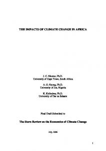
3 Results and discussion For a domain including all four of the study basins the hydrologic model produced complete estimates of the water budget using each GCM. These were then summarized for four periods: the base period 1961–1990, 2011–2040, 2041–2070, and 2071–2100. To illustrate the scatter among the projections and impacts using the 11 GCMs for one basin under the A2 scenario, the results for the latter two periods are plotted in Fig. 2. This shows that there is a majority of GCMs showing increased winter P, but this is quite variable among the models, while the T increases appear more consistent. In general the impact on flow of these climatic changes is that winter flows increase and late spring and early summer flows decrease, with greater disagreement among models during the transition between the two. Declining snow water equivalent (SWE) is clear, and is more severe later in the century as temperatures continue to rise.

316


Feather R at Oroville −2070 Years 2071−2100 Years 2041− Precip,mm

400 300 200 100

Temp,oC

0

20

10

Flow,m3s−1

0

30000

20000

10000

SWE,mm

0 200

cnrm csiro gfdl giss inmcm ipsl miroc mpi mri pcm hadcm3 obs

160 120 80 40 0

J

F

M

A

M

J

J

A

S

O

N

D

J

F

M

A

M

J

J

A

S

O

N

D

Fig. 2 For one basin, for the SRESA2 scenario, the average precipitation and temperature, streamflow at the outlet point, and basin average snow water equivalent averaged over two 30-year periods. The thicker line labeled obs represents the baseline average for 1961–1990

3.1 Precipitation and temperature changes To verify the observations above, and to use both emissions scenarios, Figs. 3 and 4 are shown. Note that the confidence thresholds highlighted in the Figures are comparable to the National Assessment Synthesis Team (2000) classification of “very likely or very probable” impacts as those with confidence >90%; the 67–90% category corresponds to “likely or probable” impacts. Since the changes in P were found to be remarkably consistent between basins, only the northern and southernmost basins are included in this section. Note that Fig. 3 shows the ensemble mean changes corresponding to the scatter of GCM traces in the top row of panels in Fig. 2. The figures show for each month the mean P of the 1961–1990 base period and the change to each of the three future periods. Not shown in the figures is annual average P,


317

which exhibits small (about 5%) but significant (with 67–90% confidence) increases under the B1 emissions scenario in 2011–2040 and comparable decreases for 2041–2070. For all other cases, no statistically significant change in annual P is evident, though a pattern exists of slight increases in the north declining to slight decreases in the south. On a monthly level, Fig. 3 generally shows an increase in December–February P. A significant decline in April–June P is projected, and grows in magnitude later in the century, and the increase in winter P persists. Figure 4 shows a similar pattern toward the south, though with sharper declines in April–June P than in the north, and smaller increases in winter P especially later in the twenty-first century. Overall, the increase in winter P and decrease in spring P shifts the centroid of the annual precipitation volume 2–6 days earlier by 2071–2100. While not shown, the T projections in the north and south are very close and are highly significant, even as early as 2011–2040. By the end of the twenty-first century, average annual T rises by 3.6–3.8°C for the A2 scenario, and 2.3–2.4°C for B1, with the greatest warming being in July with 3.0–3.1°C for the B1 scenario and 5.0–5.1°C for A2. While these changes are broad in scale, showing high consistency between the north and south, the differing characters of the basins produces different hydrologic responses. To assess the separation of the future climate under the two SRES scenarios, the same statistical test for equality of means is performed between the A2 and B1 scenarios for 2071–2100. While both scenarios show highly significant changes in T by the end of the century, it is also found that the T rises are smaller for B1 as compared to A2 with statistical confidence exceeding 90% (with the exception of March for basins 2 and 4, where confidence is 87–88% that they differ). Differences in P projected under the two scenarios

Basin 1 Precipitation Changes Precip,mm/d

8

6

4

2

A2_ΔP,mm/d

0

B1_ΔP,mm/d

Fig. 3 Mean monthly precipitation and projected changes under the A2 and B1 emission scenarios for Basin 1 (see Table 1 for basin description). The upper panel is the base period (1961–1990) mean monthly precipitation. The lower two panels show three bars for each month, indicating mean changes relative to the base period for 2011–2040 (left bar), 2041–2070 (center bar), and 2071–2100 (right bar). Shading indicates the statistical confidence of the change using a Mann– Whitney U test

2 1 0 −1

2 1 0 −1