The estimation of variance-covariance matrices in situations that involve the optimization of an ob- jective function (e.g. a log-likelihood function) is usually a ...
Unconstrained Parameterizations for Variance-Covariance Matrices Jose´ C. Pinheiro and Douglas M. Bates Department of Biostatistics Department of Statistics University of Wisconsin — Madison The estimation of variance-covariance matrices in situations that involve the optimization of an objective function (e.g. a log-likelihood function) is usually a difficult numerical problem, since the resulting estimates should be positive semi-definite matrices. We can either use constrained optimization, or employ a parameterization that enforces this condition. We describe here five different parameterizations for variance-covariance matrices that ensure positive definiteness, while leaving the estimation problem unconstrained. We compare the parameterizations based on their computational efficiency and statistical interpretability. The results described here are particularly useful in maximum likelihood and restricted maximum likelihood estimation in mixed effects models, but are also applicable to other areas of statistics. KEY WORDS: Unconstrained estimation, Variance-covariance components estimation, Cholesky factorization, matrix logarithm.
1.
I NTRODUCTION
The estimation of variance-covariance matrices through optimization of an objective function, such as a log-likelihood function, is usually a difficult numerical problem, since one must ensure that the resulting estimate is positive semi-definite. This kind of estimation problem occurs, for example, in the analysis of linear and nonlinear mixed-effects models, when one is interested in obtaining maximum likelihood, or restricted maximum likelihood, estimates of the random effects variance-covariance matrix (Lindstrom and Bates, 1988 and 1990). In these models, because the random effects are unobserved quantities, no sample variance-covariance matrix type of estimator, that would automatically be positive semi-definite, is available. Indirect estimation methods must be used. The estimation of a variancecovariance matrix through optimization of a log-likelihood function may occur even when a sample variance-covariance estimator is available, if, for example, one is interested in using maximum likelihood asymptotic results to assess the variability in the resulting estimates. Two approaches can be used to ensure positive semidefiniteness of a variance-covariance matrix estimate: constrained optimization, where the natural parameterization for the upper-triangular elements in the variance-covariance matrix is used and the estimates are constrained to be positive semidefinite matrices; and unconstrained optimization, where the upper-triangular elements in the variance-covariance matrix are reparameterized in such way that the resulting estimate must be positive semi-definite. The first approach, constrained optimization using the nonredundant entries of the matrix as parameters, would be very difficult. As Dennis, Jr. and Schnabel (1983) point out, attempts to solve a constrained optimization problem usually boil down to repeated unconstrained problems or to solving a nonlinear system of equations. The simplest cases are those where there are simple inequality constraints on the parameters and even in those cases constrained solutions can require several times as much
�
effort as an unconstrained solution. In addition, the statistical properties of constrained estimates, such as asymptotic properties, can be difficult to characterize. In this case, the constraints themselves are quite complicated to express. Verifying that a given symmetric matrix is positive semi-definite is essentially as difficult as employing one of the unconstrained parameterizations we will describe later. For these reasons, we recommend the use of unconstrained optimization with a parameterization that enforces the positive semi-definite constraint. An unconstrained estimation approach for variancecovariance matrices in a Bayesian context using matrix logarithms can be found in Leonard and Hsu (1993). Lindstrom and Bates (1988, 1990) describe the use of Cholesky factors for implementing unconstrained estimation of random effects variance-covariance matrices in linear and nonlinear mixed effects models using likelihood and restricted likelihood. Since a variance-covariance matrix is positive semi-definite, but not positive definite, only in the rather degenerate situation of linear combinations of the underlying random variables taking constant values, we will restrict ourselves here to positive definite variance-covariance matrices. In addition to enforcing the positive definiteness constraints, the choice of the parameterization can be influenced by computational efficiency and by the statistical interpretability of the individual elements. In general, we can use numerically or analytically determined second derivatives of the objective function to approximate standard errors and derive confidence intervals for the individual parameters. To assess the variability of the variances and covariances estimates, it is desirable that they can be expressed as simple functions of the unconstrained parameters. More detailed techniques, such as profiling the likelihood (Bates and Watts, 1988, chapter 6), also work best for functions of the variance-covariance matrix that are expressed in the original parameterization. We describe in Section 2 five different parameterizations for
U NCONSTRAINED PARAMETERIZATIONS
FOR
VARIANCE -C OVARIANCE M ATRICES
transforming the estimation of unstructured (general) variancecovariance matrices into an unconstrained problem. In Section 3 we compare the parameterizations with respect to their computational efficiency and statistical interpretability. Our conclusions and suggestions for further research are presented in Section 4.
2.
PARAMETERIZATIONS
�
Let denote a symmetric positive definite n � n variancecovariance matrix corresponding to a random vector = (X1 ; : : : ; Xn ). We do not assume any further structure for . Because is symmetric, only n(n +1)=2 parameters are needed to represent it. We will denote by any such minimal set of parameters to determine . The rationale behind all parameterizations considered in this section is to write
X
�
�
�
�
�=L L (2.1) where L = L (�) is an n � n matrix of full rank obtained from a n(n + 1)=2-dimensional vector of unconstrained parameters �. It is clear that any � defined from a full rank L as in (2.1) is
Another problem with the Cholesky parameterization is the lack of a straightforward relationship between and the elements of . This makes it hard to interpret the estimates of and to obtain confidence intervals for the variances and covariances in based on confidence p intervals for the elements of . One exception is j[ ]11 j = [ ]11 , so confidence intervals on [ ]11 can be obtained from confidence intervals on [ ]11 , where [ ]ij denotes the ij th element of the matrix . By appropriately permuting the columns and rows of we can in fact derive confidence intervals for all the variance terms based on confidence intervals for the elements of . The main advantage of this parameterization, apart from the fact that it ensures positive definiteness of the estimate of , is that it is computationally simple and stable. The Cholesky factorization of in (2.2) is
L
�
L
�
�
�
�
�
2 3 1 1 1 A=4 1 5 5 5 1 5 14
(2.2)
�
�
is positive definite, it may by factored as = Because T , where is an upper triangular matrix. Setting to be the upper triangular elements of gives the Cholesky parameterization of . Lindstrom and Bates (1988) use this parameterization to obtain derivatives of the log-likelihood of a linear mixed effects model for use in a Newton-Raphson algorithm. They reported that the use of this parameterization dramatically improved the convergence properties of the optimization algorithm, when compared to a constrained estimation approach. One problem with the Cholesky parameterization is that the Cholesky factor is not unique. In fact, if is a Cholesky factor of then so is any matrix obtained by multiplying a subset of the rows of by ?1. This has implications on parameter identification, since up to 2n different may represent the same . Numerical problems can arise in the optimization of an objective function when different optimal solutions are close together in the parameter space.
LL
L
�
�
�
L
L
L
�
�
L
�
�
A
A
�
� �
L
L
�
A
2 32 3 1 0 0 1 1 1 A = 4 1 2 0 54 0 2 2 5 1 2 3 0 0 3
By convention, the components of the upper triangular part of T are listed column-wise to give = (1; 1; 2; 1; 2; 3) .
�
2.2 Log-Cholesky Parameterization
L
L
If one requires the diagonal elements of in the Cholesky is unique. To avoid confactorization to be positive then strained estimation, one can use the logarithms of the diagonal elements of . We call this parameterization the log-Cholesky parameterization. It inherits the good computational properties of the Cholesky parameterization, but has the advantage of being uniquely defined. As in the Cholesky parameterization the parameters lack direct interpretation in terms of the original variances and covariances, except for L11 . The log-Cholesky parameterization of is
L
L
A
� = (0; 1; log(2); 1; 2; log(3))T : 2.3 Spherical Parameterization The purpose of this parameterization is to combine the computational efficiency of the Cholesky parameterization with direct interpretation of in terms of the variances and correlations in . Let i denote the ith column of in the Cholesky factorization of and i denote the spherical coordinates of the first i elements of i . That is
�
2.1 Cholesky Parameterization
�
� �
T
positive definite. Different choices of lead to different parameterizations of . We will consider here two classes of : one based on the Cholesky factorization (Thisted, 1988, x3�3) of and another based on the spectral decomposition of (Rao, 1973, x1c�3). The first three parameterizations presented below use the Cholesky factorization of , while the last two are based on its spectral decomposition. In some of the parameterizations there are particular components of the parameter vector that have meaningful statistical interpretations. These can include the eigenvalues of , which are important in considering when the matrix is ill-conditioned, the individual variances or standard deviations, and the correlations. The following variance-covariance matrix will be used throughout this section to illustrate the use of the various parameterizations.
2
�
L
�
L
L
l
[Li ]1 = [li ]1 cos ([li ]2 ) [Li ]2 = [li ]1 sin ([li ]2 ) cos ([li ]3 )
���
[Li ]i?1 = [li ]1 sin ([li ]2 ) � � � cos ([li ]i ) [Li ]i = [li ]1 sin ([li ]2 ) � � � sin ([li ]i )
l
l
It then follows that �ii = [ i ]1 and �1i = cos([ i ]2 ); i = 2; : : : ; n, where �ij denotes the correlation coefficient between Xi and Xj . The correlations between other variables can be expressed as linear combinations of products of sines and cosines of the elements in 1 ; : : : ; n , but the relationship is not as straightforward as those involving X1 . If confidence intervals are available for the elements of i ; i = 1; : : : ; n then we can
l
2
l
l
U NCONSTRAINED PARAMETERIZATIONS
VARIANCE -C OVARIANCE M ATRICES
FOR
also obtain confidence intervals for the variances and the correlations �1i . By appropriately permuting the rows and columns of , we can in fact obtain confidence intervals for all the variances and correlations of X1 ; : : : ; Xn . The exact same reasoning can be applied to derive profile traces and profile contours (Bates and Watts, 1988) for variances and correlations of X1 ; : : : ; Xn based on a likelihood function. To ensure uniqueness of the spherical parameterization we must have
The matrix logarithm of
Unconstrained estimation is obtained by defining
� as follows
�
2.4 Matrix Logarithm Parameterization This and the next parameterization are based on the spectral decomposition of . Because is positive definite, it has n positive eigenvalues . Letting U denote the orthogonal matrix of orthonormal eigenvectors of and = diag ( ), we can write
�
By setting
� � � � = U �U T
�
(2.3)
L = � = UT 1 2
�
(2.4)
1=2 denotes the diagonal matrix with [�1=2 ]ii = in p(2.1), where [�]ii , we get a factorization of based on the spectral decomposition. is defined as log ( ) = The matrix logarithm of log ( ) T , where log ( ) = diag [log ( )]. Note that and log ( ) share the same eigenvectors. The matrix log ( ) can take any value in the space of n � n symmetric matrices. Letting be equal to its upper triangular elements gives the matrix logarithm parameterization of . The matrix logarithm parameterization defines a one-to-one mapping between and and therefore does not have the identification problems of the Cholesky factorization. It does involve considerable calculations, as produces log ( ) whose eigenstructure must be determined before in (2.4) can be calculated. Similarly to the Cholesky and log-Cholesky parameterizations, the vector in the matrix logarithm parameterization does not have a straightforward interpretation in terms of the original variances and covariances in . We note that even though the matrix logarithm is based on the spectral decomposition of , there is not a straightforward relationship between and the eigenvalues-eigenvectors of
U
�
� � �
�U �
�
�
�
�
�
�
�
�
L
�
�
�
�
�
� = (?0:174; 0:392; 1:265; 0:104; 0:650; 2:492) : 2.5 Givens Parameterization
�
The eigenstructure of contains valuable information for determining whether some linear combination of X1 ; : : : ; Xn could be regarded as nearly constant. This is useful, for example, in model building for mixed-effects models, as near zero eigenvalues may indicate overparameterization (Pinheiro and Bates, 1995). The Givens parameterization uses the eigenvalues of directly in the definition of the parameter vector . The Givens parameterization is based on the spectral decomposition of given in (2.3) and the fact that the eigenvector matrix can be represented by n(n ? 1)=2 angles, used to generate a series of Givens rotation matrices (Thisted, 1988, x3�1�6�6) whose product reproduce as follows
U
� = (0; log(5)=2; log(14)=2; ?0:608; ?0:348; ?0:787)T : �
A is
T
�
�
The spherical parameterization has about the same computational efficiency as the Cholesky and log-Cholesky parameterizations, is uniquely defined, and allows direct interpretability of in terms of the variances and correlations in . The spherical parameterization of is
A
and therefore the matrix logarithm parameterization of
�
�i = log ([li ]1 ) ; i = 1; : : : ; n and �n+(i?2)(i?1)=2+(j?1) = ! [li ]j log � ? [l ] ; i = 2; : : : ; n; j = 2; : : : ; i i j
�
A is
2 3 ?0:174 0:392 0:104 log (A) = 4 0:392 1:265 0:650 5 0:104 0:650 2:492
�
[li ]1 > 0; i = 1; : : : ; n and [li ]j 2 (0; �) ; i = 2; : : : ; n; j = 2; : : : ; i
3
�
U U = G G � � � Gn n? = ; where 8 > > > cos(�i ); if j = k = m (i) 1
2
(
1) 2
1
> or j = k = m2 (i) > > > < sin(�i ); if j = m1 (i); k = m2 (i) Gi [j; k] = > ? sin(�i ); if j = m2(i); k = m1(i) > 1; if j = k 6= m1 (i) > > > > and j = k 6= m2 (i) > > : 0; otherwise and m1 (i) < m2 (i) are integers taking values in f1; : : : ; ng and satisfying i = m2 (i) ? m1 (i)+(m1 (i) ? 1) (n ? m1 (i)=2). To ensure uniqueness of the Givens parameterization we must have
�i 2 (0; �) ; i = 1: : : : ; n(n ? 1)=2.
The spectral decomposition (2.3) is unique up to a reorderand columns of and up ing of the diagonal elements of to switching of signs in each column of . Uniqueness can be achieved by forcing the eigenvalues to be sorted in ascending order. This can be attained, within an unconstrained estimation framework, by using a parameterization suggested by Jupp (1978) and defining the first n elements of as
�
U
U
�
�i = log (�i ? �i?1 ) ; i = 1; : : : ; n where �i denotes the ith eigenvalue of � is ascending order and with the convention that �0 = 0. The remaining elements of � in the Givens parameterization are defined by the relation
� � � �n+i = log � ?i � ; i = 1; : : : ; n(n ? 1)=2 i
The main advantage of this parameterization is that the first n elements of give information about the eigenvalues of directly. Another advantage of the Givens parameterization is that it can be easily modified to handle general (not necessarily positive definite) symmetric matrices. The only modification needed is to set �1 = �1 and
�
�i = � 1 +
�
i X j =2
exp (�i ) ; i = 2; : : : ; n
VARIANCE -C OVARIANCE M ATRICES
�
U
C OMPARING
THE
Structure I
L�
�
�
�
Structure I II III
Eigenvalues
f1; 1; : : : ; 1; 1g
Givens
Structure II 6.30
1.80
1.80
0.50
0.50
0.15
0.15
0.04
0.04
Structure III
Structure IV
6.30
6.30
1.80
1.80
0.50
0.50
0.15
0.15
0.04
0.04
Structure V
Structure VI
6.30
6.30
1.80
1.80
0.50
0.50
0.15
0.15
0.04
0.04 24
43
62
81
100
5
24
Dimension
PARAMETERIZATIONS
In this section we compare the parameterizations described in Section 2 in terms of their computational efficiency and the statistical interpretability of the individual parameters. The computational efficiency of the different parameterizations is assessed by simulation. First we analyze the average time needed to calculate ( ) from for each parameterization and for different eigenstructures and for varying sizes of . Then we compare the performance of the different parameterizations in computing the maximum likelihood estimate of the variancecovariance matrix in a linear mixed effects model (Laird and Ware, 1982). on the To investigate the effect of the eigenstructure of computational efficiency of the parameterizations, six different eigenvalue structures, described in Table 1, were considered in the simulation study presented below.
Matrix Log
6.30
5
3.
Spherical
Time (seconds)
� = (?0:275; 0:761; 2:598; ?0:265; ?0:562; ?0:072)T :
Log-Cholesky
Time (seconds)
A
Cholesky
Time (seconds)
�
� �
4
Time (seconds)
The main disadvantage of this parameterization is that it involves considerable computational effort in the calculation of from the parameter vector . Another problem with the Givens parameterization is that one cannot relate to the elements of in a straightforward manner, so inferences about variances and covariances require indirect methods. The eigenvector matrix in (2.3) can also be expressed as a product of a series of Householder reflection matrices (Thisted, 1988, x3�1�2) and these in turn can be derived from n(n ? 1)=2 parameters used to obtain the directions of the Householder reflections (Pinheiro, 1994). This Householder parameterization is essentially equivalent to the Givens parameterization in terms of statistical interpretability, but it is less efficient, since the derivation of the Householder reflection matrices involves even more computation than the Givens rotations. We have not considered it here. The Givens parameterization of is
Time (seconds)
FOR
Time (seconds)
U NCONSTRAINED PARAMETERIZATIONS
43
62
81
100
Dimension
Figure 1: Average user time to calculate L as a function of n, for the different parameterizations and eigenstructures of .
�
2. Generate n independent random variables X1 ; : : : ; Xn , such that Xi � N (log (�i ) ; 0:01), and form a diagonal matrix of random eigenvalues, , with [ ]ii = exp (Xi ). This ensures that the relative variability of the random eigenvalues is the same.
�
3. Obtain
�
� = U �U T .
L
To evaluate the average time needed to calculate , we generated, for each of the eigenvalue structures in Table 1, 25 random n � n matrices according to the above algorithm, with n varying from 6 to 100. For each we obtained and recorded the average time to calculate . The time quoted is the time the CPU spent evaluating the user’s program for the calculation. Because these user times were too small for accurate evaluation when using matrices of dimension less than 10, we used 5 evaluations of for each user time calculation. Figure 1 presents the average user time as a function of n for each of the parameterizations of and for each of the eigenvalue structures in Table 1. The computational performances of the parameterizations are essentially the same for all eigenvalue structures considered. The Cholesky, the log-Cholesky, and the spherical parameterizations have similar performances, considerably better than the other two parameterizations. The Cholesky and the logCholesky parameterizations have slightly better performances than the spherical parameterization, especially for n � 25. The matrix logarithm had the worst performance, followed by the Givens parameterization. These results are essentially reflecting the computational complexity of each parameterization, as described in Section 2. To compare the different parameterizations in an estimation context, we conducted a small simulation study using the linear mixed effects model
�
L
�
�
L
f1000; 1; 1; : : :; 1; 1g f1; 1; : : :; 1; 0:001g
9 8 > > = < ; 0 : 001 ; : : :; 0 : 001 IV 1000 ; : : :; 1000 {z }> > ; :| n{z=2 } | n=2 V f1000; 1; : : :; 1; 0:001g VI f10; 20; 30; : : :; (n ? 1) � 10; n � 10g Table 1: Different eigenvalue structures for n � n matrices � used
in the simulation study.
�
Random matrices of dimension n, for a given eigenvalue structure (�1 ; : : : ; �n ), were generated according to the following algorithm.
U
uni1. Select a random n-dimensional orthogonal matrix formly on the group of orthogonal matrices, using the algorithm proposed by Anderson, Olkin and Underhill (1987).
�
yi = X i ( + bi ) + �i; i = 1; : : : ; M
(3.1)
User Time to Convergence
o
o o o o o o o o o
40
o o o o
45
o o o o
20
135
o
o
o o o o
o o o o
Number of Iterations to Convergence
o
o o o o o
o o o
840 User Time (seconds)
o o o o
User Time (seconds)
o
5
User Time to Convergence 1200
o
o o
User Time (seconds)
VARIANCE -C OVARIANCE M ATRICES
Number of Iterations to Convergence 90
o
70
FOR
20
95
o
o
User Time (seconds)
U NCONSTRAINED PARAMETERIZATIONS
o
575
o o
o
70
o
50 400
10
10
o
o o
o
5.5
o
logCholesky
Spherical
Matrix log
Givens
Cholesky
logCholesky
Pameterization
Spherical
Matrix log
Givens
logCholesky
where the i are independent, identically distributed random effects with common N ( ; � 2 ) distribution and the i are independent and identically distributed error terms with common distribution Nni ( ; � 2 ), independent of the i , with ni representing the number of observations on the ith cluster. Lindstrom and Bates (1988) have shown that the log-likelihood in (3.1) can be profiled to produce a function of alone. In the simulation, we used matrices of dimensions 3 and 6. These were defined such that the nonzero elements of the ith column of the corresponding Cholesky factor were equal to the integers between 1 and i. For n = 3 we have = , as given in (2.2). For n = 3 we used M = 10, ni = 15; i = 1; : : : ; 10, �2 = 1, and = (10; 1; 2)T , while for n = 6 we used M = 50, ni = 25; i = 1; : : : 50, �2 = 1, and = (10; 1; 2; 3; 4; 5)T . In both cases, the elements of the first column of were set equal to 1 and the remaining elements were independently generated according to a U (1; 20) distribution. A total of 300 and 50 samples were generated respectively for n = 3 and n = 6, and the number of iterations and the user time to calculate the maximum likelihood estimate of for each parameterization recorded. Figures 2 and 3 present box-plots of the number of iterations and of the user times for the various parameterizations. The Cholesky, the log-Cholesky, the spherical, and the matrix logarithm parameterizations had similar performances for n = 3, considerably better than the Givens parameterization. For n = 6 the Cholesky and the matrix logarithm parameterizations gave the best performances, followed by the log-Cholesky and spherical parameterizations, all considerably better than the Givens parameterization. Because is relatively small in these examples, the numerical complexity of the different parameterizations did not play a major role in their performances. It is interesting to note that even though the matrix logarithm is the least efficient parameterization in terms of numerical complexity, it had the best performance in terms of number of iterations and user time to obtain the maximum likelihood estimate of , suggesting that this parameterization is most numerically stable. Another important aspect in which the parameterizations should be compared is their behavior as approaches singularity. All parameterizations described in Section 2 require to be positive definite, though the Givens parameterization can be modified to handle general symmetric matrices. It is usually an important statistical issue to test whether is of less than full rank, in which case the dimension of the parameter space can be
�
0 �
0 I
b
�
�
� A
X
�
�
�
�
�
�
Spherical
Matrix log
Givens
Cholesky
o
logCholesky
Pameterization
�
Cholesky
Pameterization
Figure 2: Box-plots of user time and number of iterations to convergence for 300 random samples of model (3.1) with of dimension 3.
b
o
35 o
275
5 Cholesky
o
o o
o
Spherical
Matrix log
Givens
Pameterization
Figure 3: Box-plots of user time and number of iterations to convergence for 50 random samples of model (3.1) with of dimension 6.
�
reduced. As approaches singularity its determinant goes to zero and so at least one of the diagonal elements of its Cholesky factor goes to zero too. The Cholesky parameterization would then become numerically unstable, since equivalent solutions would get closer together in the estimation space. At least one element of in the log-Cholesky parameterization would go to ?1 (the logarithm of the diagonal element of that goes to zero). In the spherical parameterization we would also have at least one element of going in absolute value to 1: if the first diagonal element of goes to zero, �1 ! ?1; otherwise at least one angle of the spherical coordinates of the column of whose diagonal element approaches 0 would either approach 0 or � , in which cases the corresponding element of would go respectively to ?1 or 1. implies that at least one of its eigenvalues Singularity of is zero. The Givens parameterization would then have at least the first element of going to ?1. To understand what happens with the matrix logarithm parameterization when approaches singularity we note that letting (�1 ; 1 ); : : : ; (�n ; n ) represent the eigenvalue-eigenvector pairs corresponding to P we can write = ni=1 �i i Ti . As �1 ! 0 all entries of log( ) corresponding to nonzero elements of 1 T1 would converge in absolute value to 1. Hence in the matrix logarithm parameterization we could have all elements of going either to ?1 of 1 as approached singularity. Finally we consider the statistical interpretability of the parameterizations of . The least interpretable parameterization is the matrix logarithm — none of its elements can be directly related to the individual variances, covariances, or eigenvalues of . The Cholesky and log-Cholesky parameterizations have the first component directly related to the variance of X1 , the first underlying random variable in . By permuting the order of the random variables in the definition of , one can derive measures of variability and confidence intervals for all the variances in , from corresponding quantities obtained for the parameters in the Cholesky or log-Cholesky parameterizations. The Givens parameterization is the only one considered here that uses the eigenvalues of directly in the definition of . It is a very useful parameterization for identifying ill-conditioning of . None of its parameters, though, can be directly related to the variances and covariances in . Finally, the spherical parameterization is the one that gives the largest number of interpretable parameters
�
�
L
� L
L
�
�
�
�
u
�
uu
�
uu �
�
�
�
�
�
�
�
�
�
�
u
�
U NCONSTRAINED PARAMETERIZATIONS
FOR
VARIANCE -C OVARIANCE M ATRICES
of all parameterizations considered here. Measures of variability and confidence intervals for all the variances in and the correlations with X1 can be obtained from the corresponding quantities calculated for . By permuting the order of the underlying random variables in the definition of , one can in fact derive measures of variability and confidence intervals for all the variances and correlations in .
�
�
4.
�
6
R EFERENCES Anderson, T. W., Olkin, I. and Underhill, L. G. (1987). Generation of random orthogonal matrices, SIAM J. on Scientific and Stat’l. Computing 8(4): 625–629.
�
Bates, D. M. and Watts, D. G. (1988). Nonlinear Regression Analysis and Its Applications, Wiley, New York.
C ONCLUSIONS
Dennis, Jr., J. E. and Schnabel, R. B. (1983). Numerical Methods for Unconstrained Optimization and Nonlinear Equations, Prentice-Hall, Englewood Cliffs, NJ.
The parameterizations described in Section 2 allow the estimation of variance-covariance matrices using unconstrained optimization. This has numerical and statistical advantages over constrained optimization, since the latter is usually a much harder numerical problem. Furthermore unconstrained estimates tend to have better inferential properties. Of the five parameterizations considered here, the spherical parameterization presents the best combination of performance and statistical interpretability of individual parameters. The Cholesky and log-Cholesky parameterizations have comparable performances, similar to the spherical parameterization, but lack direct parameter interpretability. The Givens parameterization is considerably less efficient than these parameterizations, but has the feature of being directly based on the eigenvalues of the variance-covariance matrix. This can be used, for example, to identify nonrandom linear combinations of the underlying random variables. The matrix logarithm parameterization is very inefficient as the dimension of the variance-covariance matrix increases, but seems to be most stable parameterization. It also lacks direct interpretability of its parameters. Different parameterizations can be used at different stages of the data analysis. The matrix logarithm parameterization seems to be the most efficient for the optimization step, at least for moderately large . The spherical parameterizations is probably the best one to derive measures of variability and confidence intervals for the elements of , while the Givens parameterization is the most convenient to investigate rank deficiency of . Only unstructured variance-covariance matrices were considered here but in many situations that involve the optimization of an objective function, structured matrices are used instead (Jennrich and Schluchter, 1986). It is therefore important to derive parameterizations for structured variance-covariance matrices that allow unconstrained estimation of the associated parameters. The asymptotic properties of the different parameterizations considered here have not yet been studied and certainly constitute an interesting research topic. It may be that some of the parameterization give faster rates of convergence to normality than others and this could be used as a criterion for choosing among them.
�
�
�
ACKNOWLEDGEMENTS This research was partially supported by the National Science Foundation through grant number DMS-9309101 and by the Coordenac¸a˜ o para Aperfeic¸oamento de Pessoal de N´ıvel Superior, Brazil. We are grateful to Bruce E. Ankenman for suggesting the Givens parameterization and to two anonymous referees for helpful comments and suggestions.
Jennrich, R. I. and Schluchter, M. D. (1986). Unbalanced repeated measures models with structural covariance matrices, Biometrics 42(4): 805–820. Jupp, D. L. B. (1978). Approximation to data by splines with free knots, SIAM Journal of Numerical Analysis 15(2): 328– 343. Laird, N. M. and Ware, J. H. (1982). Random-effects models for longitudinal data, Biometrics 38: 963–974. Leonard, T. and Hsu, J. S. J. (1993). Bayesian inference for a covariance matrix, Annals of Statistics 21: 1–25. Lindstrom, M. J. and Bates, D. M. (1988). Newton-Raphson and EM algorithms for linear mixed-effects models for repeated-measures data, Journal of the American Statistical Association 83: 1014–1022. Lindstrom, M. J. and Bates, D. M. (1990). Nonlinear mixed effects models for repeated measures data, Biometrics 46: 673–687. Pinheiro, J. C. (1994). Topics in Mixed Effects Models, PhD thesis, University of Wisconsin–Madison. Pinheiro, J. C. and Bates, D. M. (1995). Model building for nonlinear mixed-effects models, Technical Report 91, Department of Biostatistics, University of Wisconsin – Madison. Rao, C. R. (1973). Linear statistical inference and its applications, 2nd edn, Wiley, New York. Thisted, R. A. (1988). Elements of Statistical Computing, Chapman & Hall, London.