The computer used for the video processing mounts an. Intel Xeon E5-2609 2.5 Ghz 10Mb cache Ivy Bridge Pro- cessor, 16Gb DDR3 SDRAM and a PNY ...
UNCOOPERATIVE OBJECTS POSE, MOTION AND INERTIA TENSOR ESTIMATION VIA STEREOVISION M. Lavagna1 , V. Pesce1 , and R. Bevilacqua2 1
Politecnico di Milano, Aerospace Science and Technology Dept, Via La Masa 34, 20156 Milano, Italy 2 University of Florida, 32611 Gainesville, USA
ABSTRACT Autonomous close proximity operations are an arduous and attractive problem in space mission design. In particular, the estimation of pose, motion and inertia properties of an uncooperative object is a challenging task because of the lack of available a priori information. In addition, good computational performance is necessary for real applications. This paper develops a method to estimate the relative position, velocity, angular velocity, attitude and inertia properties of an uncooperative space object using only stereo-vision measurements. The classical Extended Kalman Filter (EKF) and an Iterated Extended Kalman Filter (IEKF) are used and compared for the estimation procedure. The relative simplicity and low computational cost of the proposed algorithm allow for an online implementation for real applications. The developed algorithm is validated by numerical simulations in MATLAB using different initial conditions and uncertainty levels. The goal of the simulations is to verify the accuracy and robustness of the proposed estimation algorithm. The obtained results show satisfactory convergence of the estimation errors for all the considered quantities. An analysis of the computational cost is addressed to confirm the possibility of an onboard application. The obtained results, in several simulations, outperform similar works present in literature. In addition, a video processing procedure is presented to reconstruct the geometrical properties of a body using cameras. This method has been experimentally validated at the ADAMUS (ADvanced Autonomous MUltiple Spacecraft) Lab at the University of Florida.
1.
INTRODUCTION
Over the past few decades, spacecraft autonomy has become a very important aspect in space mission design. In this paper, autonomous spacecraft proximity operations are discussed with particular attention to the estimation of position and orientation (pose), motion and inertia properties of an uncooperative object. The precise pose and motion estimation of an unknown object, such as a Resident Space Object (RSO) or an asteroid has many po-
tential applications. In fact, it allows autonomous inspection, monitoring and docking. However, dealing with an uncooperative space body is a challenging problem because of the lack of available information about the motion and the structure of the target. Relative navigation between non-cooperative satellites can become a powerful tool in missions involving objects that cannot provide effective cooperative information, such as faulty or disabled satellite, space debris, hostile spacecraft, asteroids and so on. In particular, the precise pose and motion estimation of an uncooperative object has possible applications in the space debris removal field. The pose and the inertia matrix estimation is the first step to implement a system to recover and remove elements harmful to operational and active satellites. Additionally, the obtained algorithm can be installed on autonomous spacecraft for close-proximity operations to asteroids or for rendezvous manoeuvres. This work focuses on the problem of how to estimate the relative state and the inertia matrix of an unknown, uncooperative space object using only stereoscopic measurements.
2.
DYNAMICAL MODEL
The accurate description of the relative motion is a key point in space systems involving more than one object. Correct modeling of relative translational and rotational motion is essential for autonomous missions. In literature, a large number of studies about point-mass models for relative spacecraft translational motion can be found. The most famous and used model is the one presented by Clohessy and Wiltshire [1]. Usually, these models are not sufficiently accurate when the faced problem deals with multiple cooperative spacecraft. For this reason, a different model is here considered. The location of a point in a three dimensional space must be specified with respect to a reference system. An appropriate description of the used coordinate systems is provided in this section. Two objects are considered: a leader L and a target T. In this work, the leader is the inspecting spacecraft and the target is the unknown, uncooperative object. The standard Earth-centred, inertial, Cartesian right-hand reference frame is indicated with the
letter I. L is the local-vertical, local-horizontal (LVLH) reference frame. It is fixed to the leader spacecraft’s centre of mass, the ˆ x unit vector directed from the spacecraft radially outward, ˆz normal to the leader orbital plane, and ˆ y completing the frame. Then with J , a Cartesian righthand body-fixed reference frame attached to the leader spacecraft’s centre of mass is denoted. Finally T , a Cartesian right-hand body-fixed reference frame centred on the target spacecraft’s centre of mass. It is also assumed that this frame is coincident with the principal axis of inertia. In this work, the frames J and L are assumed to be aligned. From now on, only the letter L is used to refer to both of them.
by a set of non-linear ordinary differential equations. In particular: x ¨ −2ϑ˙ L y− ˙ ϑ¨L y− ϑ˙ 2L x =
µ(rL + x) [(rL +
y¨+2ϑ˙ L x+ ˙ ϑ¨L x−ϑ˙ 2L y = − z¨ = −
x)2
+
y2
+
3 z2] 2
+
µy [(rL + µz
x)2
3
+ y2 + z2 ] 2
µ rL 2 (4) (5)
(6) 3 [(rL + x)2 + y 2 + z 2 ] 2 with rL being the norm of the position vector of the leader, µ is the Earth’s gravitational constant and ρL = [x, y, z]T . ϑ˙ L and ϑ¨L are the orbital angular velocity and acceleration of the leader and are equal to r µ ϑ˙ L = (1 + eL cos ϑL )2 (7) aL 3 (1 − eL 2 )3 −2r˙L ϑ˙ L (8) ϑ¨L = rL The rotational dynamics is described exploiting the Euler equation. Combining the Euler equations for both leader and target object, the following result is obtained: L dω T T IL = IL DI−1 T [NT − ωT | × IT ωT | ] dt L L
L
L
L
− IL ωL | × ωL | − [NL − ωL | × IL ωL | ] (9) Figure 1: Leader - Target Reference Frames The notation that is used in the formulation is now presented. The vector ρ0 is the vector connecting the leader center of mass with the target center of mass, expressed in the leader frame. Analogously, ρi can be defined as the position vector, in the leader frame, between the leader center of mass and a feature point Pi on the target. Consequently, ρ˙ 0 and ρ˙ i are the translational velocities of the target centre of mass and of a generic feature point, expressed in L. The relative angular velocity is expressed as ω. This vector is the difference of the angular velocities of the leader and target respectively, expressed in the leader frame: ω = ωT |L − ωL |L (1) The relative attitude is described using the rotation quaternion q = [q0 , q1 , q2 , q3 ]T where the first component is the scalar part and the other three are the vector one. The classical formulation for the dynamical model in a Kalman Filter dealing with non-linear equations is: x˙ = f (x) + w(t)
(2)
where x is the state vector, f (x) is a non-linear function describing the process and w is a random zero-mean white noise. In our case, the state vector is defined as: x=
[ρT0 ,
ρ˙ T0 ,
T
T
T T
ω , q , Pi ]
(3)
This is a 13 + 3N elements vector where N is the number of feature points. The relative dynamics is modelled considering the translational and the rotational motions decoupled. The relative translational dynamics is described
where IL and IT are the inertia matrices of the leader and target, ωL and ωT the corresponding angular velocities, D is the rotation matrix and NL and NT are the external torque that are assumed to be zero in this case. It is also possible to describe the relative attitude kinematics, using the quaternion kinematic equations of motion: q˙ =
1 T Qω| 2
(10)
with −q1 q0 Q(q) = q3 −q2
−q2 −q3 q0 q1
−q3 q2 −q1 q0
The motion of the feature points can be defined as: i i P˙ T |L = P˙ T |T + ω × PiT |L = ω × PiT |L
(11)
This is expressed in leader frame. However, the dynamics of the feature points is simpler if expressed in the target frame. In fact, due to the rigid body assumption, a feature point cannot change its relative position with respect to the target center of mass. This leads to: i P˙ T |T = 0
(12)
Considering that the center of mass dynamics is described by eqs. (5) to (7), the position of a single feature point can be described as follows: ρi = ρ0 + PiT |L
(13)
3.
OBSERVATION MODEL
respectively. The resulting difference is called disparity and it is defined as:
The purpose of this section is to describe the observation model that allows to obtain information from the collected stereoscopic images. Suppose to have two cameras in a stereo configuration mounted on the leader spacecraft L. The center of projection of the right camera is assumed to coincide with the centre of mass of the leader. It is also the origin of the Cartesian right-hand camera frame [X, Y, Z]. The left camera is separated by a baseline b from the right camera. Using a pinhole camera model and exploiting the perspective projection model, a point in a 3D frame is described in the 2D image plane. With this method all the selected and tracked feature points are expressed in the 2D camera plane. For the line-of-sight ρi between a generic feature point and the leader centre of mass, assuming to have a focal length equal to 1, the following expressions are derived:
di = uL − uR
(20)
The disparity allows to reconstruct information about the depth. The human brain does something similar, interpreting the difference in retinal position. In stereo vision applications, this can be performed exploiting the so called triangulation. A set of feature points is chosen and it is assumed that they are always in the view of the cameras. Therefore, according to our assumptions, the initial set of points is always traceable. At each time step, the discrete measurement vector provided by the cameras is: Zi = [wRi , wLi , w˙ Ri , w˙ Li , di ]
(21)
Therefore, the observation equation is: Zi = h(x) + v(t)
(22)
with v random zero-mean white noise.
For the right camera uR (i) =
xi yi
vR (i) =
zi yi
(14)
and for the left camera
uL (i) =
xi − b yi
vL (i) =
zi yi
(15)
where ρi = [xi , yi , zi ] is expressed in the camera frame. We can also define wR = [uR vR ] and wL = [uL vL ]. Further information can be recovered from the acquired images, exploiting the optical flow. A formulation of the relation between the 3D motion and the optical flow is derived in [2]. This relationship is expressed by the following equations: � �� � 1 ρ˙ 0 w˙ R i = A(wR i ) B(wR i ) (16) ω yi and
INERTIA RATIOS ESTIMATION
For the presented model, an a priori knowledge of the target inertia matrix is necessary. This is not a realistic assumption since we are dealing with a completely unknown and uncooperative space object. To overcome this contradiction, an estimation of the basic inertial properties is necessary. A torque free motion is assumed. In this condition, the inertia matrix is not fully observable. In fact, only two of three degrees of freedom are observable. Thus, two parameters are sufficient to represent the inertia matrix. With a parametrized inertia matrix, the motion can be propagated in the correct way. However, no geometrical or mass properties can be recovered. A proper parametrization of the inertia matrix is necessary. The selected formulation is the one proposed by Tweddle [3]. In particular: � � � � Iy Ix k2 = ln (23) k1 = ln Iy Iz
�
w˙ L i
�� � 1 ρ˙ 0 = A(wL i ) B(wL i ) ω yi
4.
with
� A=
and
� B=
1 0
−w1 w2 −1 − w2 2
0 w1 1 w2
(17)
�
1 + w1 2 w1 w2
(18) −w2 w1
� (19)
where w1 and w2 are the first and the second component of the vector w. It is important to underline that, in reality, cameras collect images at a given sampling frequency. Using two subsequent frames, the optical flow can be estimated and the image velocity computed. However, in the presented observation model, it is assumed that the information about the image velocity is recovered at each time step. Another problem is to determine the different location of the same point in the left and right image plane
This formulation relies on the minimum number of parameters, equal to the number of degrees of freedom. k1 and k2 do not have any additional constraints. The inertia ratios have to be greater than zero and they can be each value up to infinite. This is a consistent parametrization because the natural logarithm has the same validity domain. Using this parametrization, the target inertia matrix can be expressed as: Ix Iy
IT = 0 0
0 1 0
0 ek1 0 = 0 Iz 0 Iy
0 0 1 0 0 e−k2
(24)
At this point, these two parameters must be estimated by the filter. Therefore, a new augmented state can be defined as: x = [ρT0 , ρ˙ T0 , ω T , qT , Pi T , k1 , k2 ]T
(25)
Also the dynamical model is different. In fact, the parametrized inertia matrix will substitute the previous value of the target inertia matrix in the rotational dynamics expression. Additionally, two equations for k1 and k2 are considered. ∂k1 =0 (26) ∂t ∂k2 =0 (27) ∂t Equation (26) and (27) are valid under the assumption of rigid body motion and without considering any mass variation. In order to improve the convergence of the filter a pseudo measurement constraint can be added. With this equality constraint, the value of the inertia matrix can be forced to converge to the correct value. In particular: 0 = ω˙ T + IT −1 (ωT × IT ωT )
(28)
This is the new pseudo measurement. It is the classical Euler equation for the rotational dynamics of the target. A fundamental aspect to take into account is that in the pseudo measurement equation, the target angular acceleration is present. Information about this quantity have to be recovered from the actual measurement. However, with knowledge of ωL , ω˙ L and ω, there is not an analytical expression independent on IT to compute ω˙ T . This implies that the angular acceleration of the target has to be measured. With the knowledge of the optical flow, the value of ω at each time step can be recovered. Then, a numerical differentiation can be performed to find the relative angular acceleration.
5.
NUMERICAL SIMULATIONS
In this section, an evaluation of the performance and robustness of the filter is presented. Monte-Carlo simulations are performed for different values of the initial error covariance and initial relative position. Each simulation is performed considering a satellite and an object in low Earth orbit. In particular, the leader orbit is known. It is assumed that the orbit of the leader has eccentricity eL = 0.05, semi-major axis aL = 7170 km, inclination iL = 15 deg, argument of the perigee ω = 340 deg and right ascension of ascending node Ω = 0 deg. According to our parametrization, the leader inertia is " # 0.83 0 0 0 1 0 IL = kg m2 (29) 0 0 1.083 In addition, two parallel cameras, in a stereo configuration and pointing in the same direction are mounted on the leader spacecraft. The baseline between the cameras is assumed equal to 1 m. Moreover, only five feature points are supposed to be measured. This is an extreme case, in fact, more than five points are usually visible and detectable. However, this condition may occur when the object is not properly illuminated or if it is too bright. Additionally, considering only a small number of points, the robustness and convergence of the filter are
tested also with poor available measurements. The detected features are assumed to be spread over the body of the target with a distance from the centre of mass in the order of 1.5 m. This can be varied according to the dimension of the target object. After defining the initial condition for the leader orbit, the state has to be initialized. The initial state vector is: x0 = [ρ0 , ρ˙ 0 , ω, q0 , PT i , k1 , k2 ]
(30)
This vector will be defined for each simulation. At this point, the filter parameters have to be selected. In particular, the covariance matrices Q, R, P have to be chosen. R represents the measurement noise and it can be determined whenever the sensor accuracy is given. In the following simulations, the measurements noise of the and of the process is modelled as a zero-mean Gaussian with standard deviation of 10−5 . Q, the process covariance matrix, has to be selected to ensure the convergence of the filter. Finally, the initial value of P, the error covariance matrix, represents the uncertainties in the initial estimation of the state. For each time step, the quaternion is normalized. According to the IEKF formulation, after the initial condition initialization, the predicted value of the state has to be computed using the dynamical model. The function ode45 is used in MATLAB to integrate the set of dynamical equations for each time step. Then, a centred difference method is used to compute the Jacobian of the process model. With this value, the transition matrix is computed and the new error covariance is predicted. At this point, a while cycle is used to implement the iterative procedure of the Iterated Extended Kalman Filter. A tolerance equal to 0.01 and a maximum number of iterations equal to 10 is used. For the observation model, the equations are solved and linearised with the same approximate method. Finally, the filter innovation, innovation covariance and gain are iteratively computed and state and covariance are updated. In our simulations, a time step of 1 second is used and the total time of the simulation is 100 seconds. The computed errors are defined as: q eρ = (ρx − ρx )2 + (ρy − ρy )2 + (ρz − ρz )2 (31) with eρ being the error of the estimation of the centre of mass. In this notation, ρ denotes the estimated value of ρ. In the same way the relative translational velocity error can be defined: q eρ˙ = (ρ˙ x − ρ˙ x )2 + (ρ˙ y − ρ˙ y )2 + (ρ˙ z − ρ˙ z )2 (32) And the relative angular velocity error: q eω = (ωx − ω x )2 + (ωy − ω y )2 + (ωz − ω z )2 (33) For k1 and k2 the error is simply: p p ek1 = (k1 − k 1 )2 ek2 = (k2 − k 2 )2
(34)
The attitude error is defined in a different way. Recalling the definition of the inverse of a quaternion: q−1 =
q∗ ||q||2
(35)
where q∗ is the conjugate of q, the error quaternion is equal to: qe = q ⊗ q−1 (36)
eθ = 2 cos−1 (qe0 )
1.6
1.4
error [m]
The symbol ⊗ is defined as the product of two quaternions. Finally, the attitude estimation error can be defined as:
ρ 1.8
IEKF
1.2
1
(37)
0.8
where in out notation, qe0 is the scalar part of the error quaternion. In the following examples, the performance of the filter is analysed.
0.6
0.4 0
10
20
30
40
50
60
70
80
90
100
Time [sec]
Figure 2: Relative Position Error- Case A 5.1.
Case A - with pseudo-measurement constraint ρ˙
10 1
IEKF
In the first case scenario, the filter is tested with the following initial conditions:
• ρ˙ 0 = [0.01, −0.0225, −0.01] m/s
error [m/s]
• ρ0 = [10, 60, 10] m
10 0
• ω0 = [−0.1, −0.1, 0.034] deg/s
10 -1
10 -2
10 -3
• q0 = [0, 0, 0, 1]
10 -4
0
10
20
30
40
50
60
70
80
90
100
Time [sec]
ω 10 1 IEKF
10 0
error [deg/s]
These values approximate the uncertainties in a real application. For this case, 100 simulations are considered. The mean relative errors after 10 seconds are evaluated according to eqs. (31) to (33) and (37). In this work, both EKF and IEKF are used. However, only the results corresponding to the IEKF are here reported. In fact, it results to perform better and to be more robust with respect to the simple Extended Kalman Filter. The presented results show robust convergence in all the analysed simulations. Very good results are obtained for the relative angular and translational velocity in fig. 3 and fig. 4. This is probably connected to the fact that the optical flow equation is exploited. The relative attitude is always difficult to estimate in a proper way and with good convergence. fig. 5 shows poor convergence of the relative angle error. The error tends to remain close to the initial value. The two inertia ratios have good convergence thanks to the imposed equality constraint, as reported in fig. 6 and fig. 7. In table 1, the results are summarized.
Figure 3: Relative Translational Velocity Error - Case A
10 -1
10 -2
10 -3
10 -4
0
10
20
30
40
50
60
70
80
90
100
Time [sec]
Figure 4: Relative Angular Velocity Error - Case A θ 1.5 IEKF
1
error [deg]
The components of the covariance matrix are chosen to represent a realistic situation. In particular, P is composed by: σρ 2 = [1, 1, 1] m2 ; σρ˙ 2 = [1, 1, 1] m2 /s2 ; σω 2 = [1, 1, 1] deg 2 /s2 ; σq 2 = [1, 1, 1, 1] · 10−5 ; σP 2 = [1, 1, 1] m2 ; σI 2 = [1, 1].
0.5
5.2.
Case B - without pseudo-measurement constraint
0 0
10
20
30
40
50
60
70
80
90
100
Time [sec]
In this case, the equality constraint is removed. Therefore the filter performance is evaluated with no precise
Figure 5: Relative Attitude Error - Case A
Table 1: State Errors - Case A Percentiles
ρ [m]
ρ˙ [m/s]
ω [deg/s]
θ [deg]
k1 [−]
k2 [−]
50 70 90 100
0.51 0.64 0.73 0.90
0.0062 0.0067 0.0073 0.011
0.0035 0.0036 0.0039 0.0043
0.49 0.61 0.77 0.87
0.067 0.13 0.24 0.53
0.037 0.051 0.23 0.23
k1
0.6
IEKF
rotational dynamics does not affect the translation. The angular velocity and attitude errors trends are comparable to the Case A outputs. The small values for the angular velocity are the reason why for these similarities. From the presented results, the inertia ratios errors seem to converge to zero. However, this is only due to the fact that the initial covariance is small. In fact, looking at the trend of the error in fig. 8 and fig. 9, it is clear how the error tends to be constant. This means that the estimated inertia ratio remains constant and does not converge.
0.5
k1 0.4
IEKF
error [-]
0.48 0.46
0.3
0.44 0.42
error [-]
0.2
0.1
0.4 0.38 0.36
0 0
10
20
30
40
50
60
70
80
90
0.34
100
Time [sec]
0.32 0.3
Figure 6: k1 Inertia Ratio Error - Case A
0.28 0
10
20
30
40
50
60
70
80
90
100
Time [sec]
knowledge about the inertia properties. The Case A initial conditions are applied :
Figure 8: Inertia Ratio Error - Case B
• ρ0 = [10, 60, 10] m
k2
0.9
IEKF
0.85
• ρ˙ 0 = [0.01, −0.0225, −0.01] m/s
0.8
• ω0 = [−0.1, −0.1, 0.034] deg/s error [-]
0.75
• q0 = [0, 0, 0, 1]
0.7 0.65 0.6
For the covariance matrix, a smaller value is assumed for the inertia ratios: σρ 2 = [1, 1, 1] m2 σρ˙ 2 = [1, 1, 1] m2 /s2 σω 2 = [1, 1, 1] deg 2 /s2 σq 2 = −5 2 2 [1, 1, 1, 1] · 10 σP = [1, 1, 1] m σI 2 = [1, 1]/2. The filter keeps being robust under these new conditions too, and almost always converges. The position and translational velocity error trends do not change. Actually the
0.55 0.5 0
10
20
30
40
50
60
70
80
90
100
Time [sec]
Figure 9: Inertia Ratio Error - Case B In table 2, the error results are summarized. Table 2: State Errors - Case B
k2
2
IEKF
1.8 1.6 1.4
error [-]
1.2
Percentiles
ρ [m]
ρ˙ [m/s]
ω [deg/s]
θ [deg]
k1 [−]
k2 [−]
50 70 90 100
0.51 0.6 0.77 0.96
0.0081 0.009 0.011 0.013
0.0058 0.0059 0.0063 0.0069
0.59 0.74 0.88 1.2
0.33 0.6 1.4 3.2
0.35 0.55 1.6 2.6
1 0.8 0.6 0.4
5.3.
0.2 0 0
10
20
30
40
50
60
70
80
90
Case C - without constraint, high angular velocity
100
Time [sec]
Figure 7: k2 Inertia Ratio Error - Case A
So far, only small values for the relative angular velocity have been considered. In this simulation, the perfor-
mance of the filter without equality constraint is evaluated in a case with larger initial relative angular velocity. In particular:
k2
0.35
IEKF
0.3
0.25
error [-]
• ρ0 = [10, 60, 10] m • ρ˙ 0 = [0.01, −0.0225, −0.01] m/s
0.2
0.15
0.1
• ω0 = [−1, −1, 0.934] deg/s 0.05
• q0 = [0, 0, 0, 1]
0 0
10
20
30
40
50
60
70
80
90
100
Time [sec]
The value of ω0 is obtained increasing the value of ωT . The covariance matrix is, as before: σρ 2 = [1, 1, 1] m2 σρ˙ 2 = [1, 1, 1] m2 /s2 σω 2 = [1, 1, 1] deg 2 /s2 σq 2 = [1, 1, 1, 1] · 10−5 σP 2 = [1, 1, 1] m2 σI 2 = [1, 1]/2 Table 3: State Errors - Case C Percentiles
ρ [m]
ρ˙ [m/s]
ω [deg/s]
θ [deg]
k1 [−]
k2 [−]
50 70 90 100
0.53 0.64 0.76 0.94
0.01 0.013 0.017 0.02
0.012 0.013 0.014 0.016
1.8 2 2.2 2.5
0.035 0.043 0.069 0.15
0.021 0.024 0.032 0.043
Table 3 shows how the estimation of the relative position and translational velocities is slightly affected by the change in the angular velocity. The relative angular velocity and primarily the relative attitude are badly affected by this change. In fact, in this case, the error in the estimation of the inertia matrix strongly affects the dynamical model propagation. Therefore, the incorrect inertia ratios lead to a decay in the estimation performance for angular velocity and attitude. However, using a larger value for the target angular velocity implies better results in the inertia ratios estimation also without the equality constraint imposed with the pseudo measurement. Figure 10 and fig. 11 show the converging trend of the inertia ratios: k1
1
IEKF
0.9 0.8 0.7
error [-]
0.6 0.5 0.4 0.3 0.2 0.1 0 0
10
20
30
40
50
60
70
80
90
100
Time [sec]
Figure 10: Inertia Ratio Error - Case C This is justified by the fact that, with a larger angular velocity, the filtering process better performs in the estimation of the inertia components. Hence, the dynamical model and the measurement equations of the angular
Figure 11: Inertia Ratio Error- Case C
velocity, force the inertia ratios to converge to a ’consistent’ and exact value. This estimation can be obtained, in torque free motion conditions, only parametrizing the inertia matrix in a proper way.
6.
INERTIA RECONSTRUCTION
In the previous section, the estimation process of the inertia ratios has been shown. However, the inertia parameters, with small relative angular velocity, are correctly recovered only if information about the angular acceleration of the target is provided. This implies to numerically derive the available measures of the angular velocity. Numerical derivatives of a quantity that is usually noisy, can introduce instabilities and produce inaccurate results. In this section, a method to recover all the inertia components is described, without relying on any numerical method. A video and image process to recover mass properties is presented. This method is not computationally efficient and, in our application, relies on free and not optimized video/image processing software. The main idea is to collect a video or images of the observed body. From this set of images, a point cloud can be constructed according to video processing algorithms. Once a point cloud is available, a triangulate mesh can be built. The mesh gives us information about the geometry of the object. At this point, an assumption has to be done. In fact, knowing the geometry, the unknown density properties of the object do not allow a complete reconstruction of the mass properties of the body. However, generalizing the problem, the density can be assumed constant. This procedure has been experimentally validate at the University of Florida to demonstrate the validity of this method also with complex geometries. A very simple experimental setup is used. The video of a 3-DOF simulator (fig. 12) are collected using a Sony HandyCam HDR-CX110. The obtained images are imported with VisualSFM [4] and the point cloud is extracted. Then, with MeshLab [5] a mesh is created. This mesh is exported to MATLAB (fig. 13) and the mass properties are recovered. The computer used for the video processing mounts an Intel Xeon E5-2609 2.5 Ghz 10Mb cache Ivy Bridge Processor, 16Gb DDR3 SDRAM and a PNY Quadro K620
2Gb Video Card. The obtained results show how the volume of the object can be reconstructed with this procedure. In particular, the resulting errors of the component of the inertia matrix are always lower than 20% with respect to the reference value. This is obtained using a CAD model of the 3-DOF simulator, imposing the same constant density.
processing procedure. In fact, the geometrical properties of a body can be reconstructed collecting multiple frames in time; the mass properties of the observed object can be then reconstructed under a uniform density distribution assumption. The step further in the research asks for the experimental campaign to validate the promising obtained numerical results and to tune the algorithms.
REFERENCES
Figure 12: 3-DOF Simulator
Figure 13: MATLAB mesh
7.
CONCLUSION
This work proposes a new algorithm for estimating the pose, motion and inertia properties of an unknown, uncooperative space object. The presented results show how the algorithm, exploiting the equality constraint, allows for a precise estimation of the complete relative state and the inertia components. Moreover a quick convergence and a satisfactory accuracy are guaranteed. Several simulations are presented to demonstrate the robustness of the algorithm with different covariance matrix values and initial conditions. Moreover, it has been shown how the inertia components, in the filtering process, can converge without the equality constraint but only with a sufficiently high value for the target angular velocity. In most of the cases, the presented algorithm shows better results with respect to similar works. A novel approach to estimate the inertia components with very limited computational burden is proposed. In addition, it has been shown how the inertia properties can be reconstructed with a video
[1] W. Clohessy, Wiltshire, ”terminal guidance system for satellite rendezvous”, 1960 [2] D. J. Heeger and A. D. Jepson, ”Subspace methods for recovering rigid motion: algorithm and implementation”, International Journal of Computer Vision, vol. 7, no. 2, pp.95-117, 1992 [3] B. E. Tweddle, ”Computer vision-based localization and mapping of an unknown, uncooperative and spinning target for spacecraft proximity operations”, PhD, Massachussets Institute of Technology, Cambridge, MA, 2013 [4] C. Wu, VisualSFM: A visual structure from motion system http://homes. cs. washington. edu/˜ ccwu/vsfm, vol.9, 2011 [5] P. Cignoni, M. Callieri, M. Corsini, M. Dellepiane, F. Ganovelli and G. Ranzuglia, Meshlab: an open-source mesh processing tool, Eurographics Italian Chapter Conference, pp.129-136, 2008 [6] S. Segal and Pini Gufil ”Stereovision-Based Estimation of Relative Dynamics Between Noncooperative Satellites: Theory and Experiments”,Control Systems Technology, IEEE Transactions, vol.22, no.2, pp 568584, 2014