Understanding Advanced Bus-Interface ... - Texas Instruments

Understanding Advanced Bus-Interface Products

SCAA029 May 1996

1

IMPORTANT NOTICE Texas Instruments (TI) reserves the right to make changes to its products or to discontinue any semiconductor product or service without notice, and advises its customers to obtain the latest version of relevant information to verify, before placing orders, that the information being relied on is current. TI warrants performance of its semiconductor products and related software to the specifications applicable at the time of sale in accordance with TI’s standard warranty. Testing and other quality control techniques are utilized to the extent TI deems necessary to support this warranty. Specific testing of all parameters of each device is not necessarily performed, except those mandated by government requirements. Certain applications using semiconductor products may involve potential risks of death, personal injury, or severe property or environmental damage (“Critical Applications”). TI SEMICONDUCTOR PRODUCTS ARE NOT DESIGNED, INTENDED, AUTHORIZED, OR WARRANTED TO BE SUITABLE FOR USE IN LIFE-SUPPORT APPLICATIONS, DEVICES OR SYSTEMS OR OTHER CRITICAL APPLICATIONS. Inclusion of TI products in such applications is understood to be fully at the risk of the customer. Use of TI products in such applications requires the written approval of an appropriate TI officer. Questions concerning potential risk applications should be directed to TI through a local SC sales office. In order to minimize risks associated with the customer’s applications, adequate design and operating safeguards should be provided by the customer to minimize inherent or procedural hazards. TI assumes no liability for applications assistance, customer product design, software performance, or infringement of patents or services described herein. Nor does TI warrant or represent that any license, either express or implied, is granted under any patent right, copyright, mask work right, or other intellectual property right of TI covering or relating to any combination, machine, or process in which such semiconductor products or services might be or are used.

Copyright  1996, Texas Instruments Incorporated

2

Contents Title

Page

Introduction . . . . . . . . . . . . . . . . . . . . . . . . . . . . . . . . . . . . . . . . . . . . . . . . . . . . . . . . . . . . . . . . . . . . . . . . . . . . . . . . . . . . . . . 1 Device Family Overview . . . . . . . . . . . . . . . . . . . . . . . . . . . . . . . . . . . . . . . . . . . . . . . . . . . . . . . . . . . . . . . . . . . . . . . . . . . . . ABT Family . . . . . . . . . . . . . . . . . . . . . . . . . . . . . . . . . . . . . . . . . . . . . . . . . . . . . . . . . . . . . . . . . . . . . . . . . . . . . . . . . . . ABTE Family . . . . . . . . . . . . . . . . . . . . . . . . . . . . . . . . . . . . . . . . . . . . . . . . . . . . . . . . . . . . . . . . . . . . . . . . . . . . . . . . . . ALVC Family . . . . . . . . . . . . . . . . . . . . . . . . . . . . . . . . . . . . . . . . . . . . . . . . . . . . . . . . . . . . . . . . . . . . . . . . . . . . . . . . . . CBT Family . . . . . . . . . . . . . . . . . . . . . . . . . . . . . . . . . . . . . . . . . . . . . . . . . . . . . . . . . . . . . . . . . . . . . . . . . . . . . . . . . . . FB Family . . . . . . . . . . . . . . . . . . . . . . . . . . . . . . . . . . . . . . . . . . . . . . . . . . . . . . . . . . . . . . . . . . . . . . . . . . . . . . . . . . . . . GTL Family . . . . . . . . . . . . . . . . . . . . . . . . . . . . . . . . . . . . . . . . . . . . . . . . . . . . . . . . . . . . . . . . . . . . . . . . . . . . . . . . . . . LV Family . . . . . . . . . . . . . . . . . . . . . . . . . . . . . . . . . . . . . . . . . . . . . . . . . . . . . . . . . . . . . . . . . . . . . . . . . . . . . . . . . . . . . LVC Family . . . . . . . . . . . . . . . . . . . . . . . . . . . . . . . . . . . . . . . . . . . . . . . . . . . . . . . . . . . . . . . . . . . . . . . . . . . . . . . . . . . LVT Family . . . . . . . . . . . . . . . . . . . . . . . . . . . . . . . . . . . . . . . . . . . . . . . . . . . . . . . . . . . . . . . . . . . . . . . . . . . . . . . . . . . LVTZ Family . . . . . . . . . . . . . . . . . . . . . . . . . . . . . . . . . . . . . . . . . . . . . . . . . . . . . . . . . . . . . . . . . . . . . . . . . . . . . . . . . .

1 1 1 1 1 2 2 2 2 2 2

Detailed Comparison . . . . . . . . . . . . . . . . . . . . . . . . . . . . . . . . . . . . . . . . . . . . . . . . . . . . . . . . . . . . . . . . . . . . . . . . . . . . . . . . 3 Input and Output Characteristics . . . . . . . . . . . . . . . . . . . . . . . . . . . . . . . . . . . . . . . . . . . . . . . . . . . . . . . . . . . . . . . . . . . . . CMOS and BiCMOS Input Characteristics . . . . . . . . . . . . . . . . . . . . . . . . . . . . . . . . . . . . . . . . . . . . . . . . . . . . . . . . . . . BiCMOS Output Characteristics (ABT and LVT) . . . . . . . . . . . . . . . . . . . . . . . . . . . . . . . . . . . . . . . . . . . . . . . . . . . . . . CMOS Output Characteristics (ALVC, LVC, and LV) . . . . . . . . . . . . . . . . . . . . . . . . . . . . . . . . . . . . . . . . . . . . . . . . . .

4 4 6 8

Incident-Wave Switching . . . . . . . . . . . . . . . . . . . . . . . . . . . . . . . . . . . . . . . . . . . . . . . . . . . . . . . . . . . . . . . . . . . . . . . . . . . . 9 GTL Input/Output Structure . . . . . . . . . . . . . . . . . . . . . . . . . . . . . . . . . . . . . . . . . . . . . . . . . . . . . . . . . . . . . . . . . . . . . . . . 10 Power Consumption . . . . . . . . . . . . . . . . . . . . . . . . . . . . . . . . . . . . . . . . . . . . . . . . . . . . . . . . . . . . . . . . . . . . . . . . . . . . . . . 13 Power Calculation . . . . . . . . . . . . . . . . . . . . . . . . . . . . . . . . . . . . . . . . . . . . . . . . . . . . . . . . . . . . . . . . . . . . . . . . . . . . . 17 Package Power Dissipation . . . . . . . . . . . . . . . . . . . . . . . . . . . . . . . . . . . . . . . . . . . . . . . . . . . . . . . . . . . . . . . . . . . . . . . . . . 18 Advanced Packaging . . . . . . . . . . . . . . . . . . . . . . . . . . . . . . . . . . . . . . . . . . . . . . . . . . . . . . . . . . . . . . . . . . . . . . . . . . . . . . . 20 Output Capacitance . . . . . . . . . . . . . . . . . . . . . . . . . . . . . . . . . . . . . . . . . . . . . . . . . . . . . . . . . . . . . . . . . . . . . . . . . . . . . . . . 22 ac Performance . . . . . . . . . . . . . . . . . . . . . . . . . . . . . . . . . . . . . . . . . . . . . . . . . . . . . . . . . . . . . . . . . . . . . . . . . . . . . . . . . . . 23 Simultaneous-Switching Phenomenon . . . . . . . . . . . . . . . . . . . . . . . . . . . . . . . . . . . . . . . . . . . . . . . . . . . . . . . . . . . . . . 23 Simultaneous-Switching Solutions . . . . . . . . . . . . . . . . . . . . . . . . . . . . . . . . . . . . . . . . . . . . . . . . . . . . . . . . . . . . . . . . 24 Slew Rate . . . . . . . . . . . . . . . . . . . . . . . . . . . . . . . . . . . . . . . . . . . . . . . . . . . . . . . . . . . . . . . . . . . . . . . . . . . . . . . . . . . . . . . . . 27 Effects of Simultaneous Switching and Capacitive Loading on Propagation Delay . . . . . . . . . . . . . . . . . . . . . . . . . . . . 31 Skew . . . . . . . . . . . . . . . . . . . . . . . . . . . . . . . . . . . . . . . . . . . . . . . . . . . . . . . . . . . . . . . . . . . . . . . . . . . . . . . . . . . . . . . . . . . . 35 Bus-Hold Circuit . . . . . . . . . . . . . . . . . . . . . . . . . . . . . . . . . . . . . . . . . . . . . . . . . . . . . . . . . . . . . . . . . . . . . . . . . . . . . . . . . . 36 Partial Power Down . . . . . . . . . . . . . . . . . . . . . . . . . . . . . . . . . . . . . . . . . . . . . . . . . . . . . . . . . . . . . . . . . . . . . . . . . . . . . . . . 37 Power-Up or Power-Down High Impedance . . . . . . . . . . . . . . . . . . . . . . . . . . . . . . . . . . . . . . . . . . . . . . . . . . . . . . . . . . . . 38 Additional Design Considerations for GTL and BTL/FB . . . . . . . . . . . . . . . . . . . . . . . . . . . . . . . . . . . . . . . . . . . . . . . . . 39 GTL . . . . . . . . . . . . . . . . . . . . . . . . . . . . . . . . . . . . . . . . . . . . . . . . . . . . . . . . . . . . . . . . . . . . . . . . . . . . . . . . . . . . . . . . 39 BTL/FB . . . . . . . . . . . . . . . . . . . . . . . . . . . . . . . . . . . . . . . . . . . . . . . . . . . . . . . . . . . . . . . . . . . . . . . . . . . . . . . . . . . . . 39

OEC, UBT, Widebus, and Widebus+ are trademarks of Texas Instruments Incorporated.

iii

Contents (continued) Title

Page

Conclusion . . . . . . . . . . . . . . . . . . . . . . . . . . . . . . . . . . . . . . . . . . . . . . . . . . . . . . . . . . . . . . . . . . . . . . . . . . . . . . . . . . . . . . . 40 Acknowledgment . . . . . . . . . . . . . . . . . . . . . . . . . . . . . . . . . . . . . . . . . . . . . . . . . . . . . . . . . . . . . . . . . . . . . . . . . . . . . . . . . . 41 References . . . . . . . . . . . . . . . . . . . . . . . . . . . . . . . . . . . . . . . . . . . . . . . . . . . . . . . . . . . . . . . . . . . . . . . . . . . . . . . . . . . . . . . . 41

List of Illustrations Figure

iv

Title

Page

1

Switching Standards With Guaranteed Thresholds . . . . . . . . . . . . . . . . . . . . . . . . . . . . . . . . . . . . . . . . . . . . . . . . . . . 4

2

Typical Input Cell for 5-V Families . . . . . . . . . . . . . . . . . . . . . . . . . . . . . . . . . . . . . . . . . . . . . . . . . . . . . . . . . . . . . . 5

3

Typical Input Cell for 3.3-V Families . . . . . . . . . . . . . . . . . . . . . . . . . . . . . . . . . . . . . . . . . . . . . . . . . . . . . . . . . . . . . 5

4

Supply Current vs Input Voltage (ABT – One Input) . . . . . . . . . . . . . . . . . . . . . . . . . . . . . . . . . . . . . . . . . . . . . . . . . 5

5

Input Characteristic Impedance of 3.3-V and 5-V Families . . . . . . . . . . . . . . . . . . . . . . . . . . . . . . . . . . . . . . . . . . . . 6

6

Typical Output Cell for 5-V Families . . . . . . . . . . . . . . . . . . . . . . . . . . . . . . . . . . . . . . . . . . . . . . . . . . . . . . . . . . . . . 7

7

Typical Output Cell for 3.3-V Families . . . . . . . . . . . . . . . . . . . . . . . . . . . . . . . . . . . . . . . . . . . . . . . . . . . . . . . . . . . . 7

8

Output-Low Characteristic Impedance of 3.3-V and 5-V Families . . . . . . . . . . . . . . . . . . . . . . . . . . . . . . . . . . . . . . 8

9

Output-High Characteristic Impedance of 3.3-V and 5-V Families . . . . . . . . . . . . . . . . . . . . . . . . . . . . . . . . . . . . . . 9

10

Reflected-Wave Switching . . . . . . . . . . . . . . . . . . . . . . . . . . . . . . . . . . . . . . . . . . . . . . . . . . . . . . . . . . . . . . . . . . . . 10

11

Typical GTL and BTL/FB Input and Output Cells . . . . . . . . . . . . . . . . . . . . . . . . . . . . . . . . . . . . . . . . . . . . . . . . . . 11

12

GTL and BTL/FB Input and Output Characteristic Impedance . . . . . . . . . . . . . . . . . . . . . . . . . . . . . . . . . . . . . . . . 12

13

Power Consumption With Single-Output Switching . . . . . . . . . . . . . . . . . . . . . . . . . . . . . . . . . . . . . . . . . . . . . . . . . 14

14

Power Consumption With All-Outputs Switching . . . . . . . . . . . . . . . . . . . . . . . . . . . . . . . . . . . . . . . . . . . . . . . . . . 15

15

FB1650 and GTL16612 Power Consumption With Single- and All-Outputs Switching . . . . . . . . . . . . . . . . . . . . . 16

16

Functional Frequency Using Standard Load Specified in Data Sheets . . . . . . . . . . . . . . . . . . . . . . . . . . . . . . . . . . . 16

17

Advanced Packages . . . . . . . . . . . . . . . . . . . . . . . . . . . . . . . . . . . . . . . . . . . . . . . . . . . . . . . . . . . . . . . . . . . . . . . . . . 19

18

Distributed Pinout of ’ABT16244A . . . . . . . . . . . . . . . . . . . . . . . . . . . . . . . . . . . . . . . . . . . . . . . . . . . . . . . . . . . . . 21

19

Cross-Section of Thermally Enhanced EIAJ 100-Pin TQFP . . . . . . . . . . . . . . . . . . . . . . . . . . . . . . . . . . . . . . . . . . 21

20

Capacitance Variation Between Families . . . . . . . . . . . . . . . . . . . . . . . . . . . . . . . . . . . . . . . . . . . . . . . . . . . . . . . . . 22

21

Simultaneous-Switching Output Model . . . . . . . . . . . . . . . . . . . . . . . . . . . . . . . . . . . . . . . . . . . . . . . . . . . . . . . . . . 23

22

Simultaneous-Switching-Noise Waveform . . . . . . . . . . . . . . . . . . . . . . . . . . . . . . . . . . . . . . . . . . . . . . . . . . . . . . . . 23

23

dc Noise Margin . . . . . . . . . . . . . . . . . . . . . . . . . . . . . . . . . . . . . . . . . . . . . . . . . . . . . . . . . . . . . . . . . . . . . . . . . . . . 24

24

Typical Output Low-Voltage Peak (VOLP) on 3.3-V and 5-V Families . . . . . . . . . . . . . . . . . . . . . . . . . . . . . . . . . . 25

25

Typical Output High-Voltage Valley (VOHV) on 3.3-V and 5-V Families . . . . . . . . . . . . . . . . . . . . . . . . . . . . . . . . 25

26

Typical Output Peak (VOLP) and Valley (VOHV) on GTL and BTL . . . . . . . . . . . . . . . . . . . . . . . . . . . . . . . . . . . . 26

27

Typical Output Rise and Fall Time Measured Between Specified Levels or Voltages . . . . . . . . . . . . . . . . . . . . . . . 27

28

Typical Output Rise and Fall Time Measured Between Specified Levels or Voltages . . . . . . . . . . . . . . . . . . . . . . . 28

29

Typical Output Rise Time as the Number of Outputs Switching Increases . . . . . . . . . . . . . . . . . . . . . . . . . . . . . . . 29

30

Typical Output Fall Time as the Number of Outputs Switching Increases . . . . . . . . . . . . . . . . . . . . . . . . . . . . . . . . 30

31

Typical Propagation Delay vs Number of Outputs Switching (Standard Load) . . . . . . . . . . . . . . . . . . . . . . . . . . . . 32

32

Typical tPHL vs Capacitive Load . . . . . . . . . . . . . . . . . . . . . . . . . . . . . . . . . . . . . . . . . . . . . . . . . . . . . . . . . . . . . . . 33

33

Typical tPLH vs Capacitive Load . . . . . . . . . . . . . . . . . . . . . . . . . . . . . . . . . . . . . . . . . . . . . . . . . . . . . . . . . . . . . . . 34

List of Illustrations (continued) Figure

Title

Page

34

Skew = |tPLH3 – tPLH4| . . . . . . . . . . . . . . . . . . . . . . . . . . . . . . . . . . . . . . . . . . . . . . . . . . . . . . . . . . . . . . . . . . . . . . . 35

35

Typical Skew Between Outputs . . . . . . . . . . . . . . . . . . . . . . . . . . . . . . . . . . . . . . . . . . . . . . . . . . . . . . . . . . . . . . . . . 35

36

Typical Bus-Hold Cell . . . . . . . . . . . . . . . . . . . . . . . . . . . . . . . . . . . . . . . . . . . . . . . . . . . . . . . . . . . . . . . . . . . . . . . . 36

37

Simplified Input Structures for CMOS and ABT Devices . . . . . . . . . . . . . . . . . . . . . . . . . . . . . . . . . . . . . . . . . . . . 37

38

Example of Partial-System Power Down . . . . . . . . . . . . . . . . . . . . . . . . . . . . . . . . . . . . . . . . . . . . . . . . . . . . . . . . . 37

39

Power-Up and Power-Down High Impedance Up to 2.1 V (ABT, FB) and 1.5 V (LVTZ) . . . . . . . . . . . . . . . . . . . 38

40

Power-Up High Impedance With Active-Low Control Pin . . . . . . . . . . . . . . . . . . . . . . . . . . . . . . . . . . . . . . . . . . . 38

41

Proposed Circuit to Generate VREF . . . . . . . . . . . . . . . . . . . . . . . . . . . . . . . . . . . . . . . . . . . . . . . . . . . . . . . . . . . . . 39

Tables Table 1

Title

Page

Input Transition Rise or Fall Rate as Specified in Data Sheets . . . . . . . . . . . . . . . . . . . . . . . . . . . . . . . . . . . . . . . . . . 6

2

ΘJA for Different Packages . . . . . . . . . . . . . . . . . . . . . . . . . . . . . . . . . . . . . . . . . . . . . . . . . . . . . . . . . . . . . . . . . . . . 20

3

List of Devices With Bus Hold . . . . . . . . . . . . . . . . . . . . . . . . . . . . . . . . . . . . . . . . . . . . . . . . . . . . . . . . . . . . . . . . . 36

4

Data-Sheet Specification for Bus Hold . . . . . . . . . . . . . . . . . . . . . . . . . . . . . . . . . . . . . . . . . . . . . . . . . . . . . . . . . . . 36

5

Summary of the Various Features and Characteristics of the Device Families . . . . . . . . . . . . . . . . . . . . . . . . . . . . . 40

v

vi

Introduction The purpose of this application report is to assist the designers of high- or low-performance digital logic systems in using the Advanced System Logic (ASL) families: LV, LVC, LVT, ALVC, ABT, ABTE, ALB, GTL, FB, and CBT. A family introduction, followed by a detailed comparison of the electrical characteristics, is provided to help designers understand the differences between these products. In addition, typical data is provided to give the hardware designer a better understanding of how these families operate under various conditions.

Device Family Overview ABT Family The ABT family is Texas Instruments (TI) second-generation family of BiCMOS bus-interface products. It is manufactured using the latest 0.8-µ BiCMOS process, and provides high drive up to 64 mA and propagation delays below the 5-ns range, while maintaining very low power consumption. ABT products are well suited for live-insertion applications with an Ioff specification of 0.1 mA. To reduce transmission-line effects, the ABT family has series-damping resistor options. Furthermore, there are special ABT parts that provide extremely high-current drive (180 mA) to transmit down to 25-Ω transmission lines. Advanced bus functions, such as universal bus transceivers (UBT ), perform a wide variety of bus-interface functions. Multiplexing options for memory interleaving and bus upsizing or downsizing also are provided. ABT devices are available in octal, Widebus, or Widebus+. Widebus and Widebus+ packages feature higher performance with reduced noise and flow-through pinout for easier board layout. In addition, Widebus+ devices have bus-hold circuitry on the inputs to eliminate the need for external pullup resistors for floating inputs. ABTE Family ABTE provides wider noise margins and is backward-compatible with existing TTL logic. ABTE devices support the VME64-ETL specification, with tight tolerances on skew and transition times. ABTE is manufactured using the latest 0.8-µ BiCMOS process and provides high drive up to 90 mA. Other features include a bias pin and internal pullup resistors on control pins for maximum live-insertion protection. Bus-hold circuitry eliminates external pullup resistors on the inputs and series-damping resistors on the outputs damp reflections. ALVC Family The highest performance 3.3-V bus-interface family is the ALVC family. These specially designed 3-V products are processed in 0.6-µ CMOS technology, giving typical propagation delays of less than 3 ns, along with current drive of 24 mA and static power consumption of 40 µA for bus-interface functions. ALVC devices have bus-hold cells on inputs to eliminate the need for external pullup resistors for floating inputs. The family also includes innovative functions for memory interleaving, multiplexing, and interfacing to synchronous DRAMs. The ALVC family is available in the Widebus footprint with advanced packaging, such as shrink small-outline package (SSOP) and thin shrink small-outline package (TSSOP). CBT Family In today’s computing market, power and speed are two of the main concerns. CBT addresses both of these issues in bus-interface applications. CBT enables a bus-interface device to function as a very fast bus switch, effectively isolating buses when the switch is open, and causing very little propagation delay when the switch is closed. These devices function as high-speed bus interfaces between computer-system components such as the central processing unit (CPU) and memory. CBT devices also can be used as 5-V to 3.3-V translators, allowing designers to mix 5-V or 3.3-V components in the same system. CBT devices are available in advanced packaging, such as SSOP and TSSOP for reduced board area.

1

FB Family The Futurebus (FB)-series devices are used for high-speed bus applications and are fully compatible with the IEEE 1194.1-1991 (BTL) standard. These transceivers are available in 7-, 8-, 9-, and 18-bit versions with TTL and BTL translation in less than 5-ns performance. Other features include drive up to 100 mA and bias pins for live-insertion applications. GTL Family GTL technology is a new reduced-voltage switching standard that provides high-speed, point-to-point communications, with low power dissipation. TI offers GTL / TTL translators to interface with the TTL-based subsystems. Designers use the GTL-switching standards for speed-sensitive subsystems, and use the translators to interface with the rest of the system. GTL devices feature innovative circuitry, such as bus hold on the TTL inputs, to eliminate the need for external pullup resistors for floating inputs, which reduces power, cost, and board-layout time. Output edge-rate control (OEC) is offered on the outputs to reduce electromagnetic interference (EMI) caused by the high frequencies of GTL. Industry-leading packaging, such as SSOP and TSSOP, is available for higher performance and reduced board space. LV Family TI’s LV CMOS technology products are specially-designed parts for 3-V power supply use with the same 5-V performance characteristics of HCMOS logic. The LV family is a 2-µ CMOS process that provides up to 8 mA of drive, and propagation delays of 18 ns maximum, while having a static power consumption of only 20 µA for both bus-interface and gate functions.The LV family is available in the octal footprint with advanced packaging, such as small-outline integrated circuit (SOIC), SSOP, and TSSOP. LVC Family TI’s LVC logic products are specially designed parts for 3-V power supply use, with about the same performance as the 5-V 74F family. The LVC family is a high-performance version with 0.8-µ CMOS process technology, 24-mA current drive, and 6.5-ns maximum propagation delays for driver operations. The LVC family includes both bus-interface and gate functions, with 50 different functions planned.The LVC family is available in the octal and Widebus footprints with advanced packaging, such as SOIC, SSOP, and TSSOP. Many LVC devices are available with 5-V tolerant inputs and outputs. LVT Family The specially designed 3-V LVT family uses the latest 0.8-µ BiCMOS process technology for bus-interface functions. Like its 5-V ABT counterpart, LVT provides up to 64 mA of drive, 4-ns propagation delays, and in addition, consumes less than 100 µA of standby power. The bus-hold feature eliminates external pullup resistors and I/Os that can handle up to 7 V, which allows them to act as 5-V/3-V translators.The LVT family is available in octal and Widebus footprints with advanced packaging, such as SOIC, SSOP, and TSSOP. LVTZ Family The LVTZ family offers all of the features found in TI’s standard LVT family. In addition, LVTZ incorporates circuitry to protect the devices in live-insertion applications. The device goes to the high-impedance state during power up and power down, which is called power-up 3-state (PU3S). The LVTZ family is available in the octal footprint with advanced packaging, such as SOIC, SSOP, and TSSOP.

2

Detailed Comparison The major subject areas covered in this application report are:

• • • • • • • • • • • • •

Input characteristics Maximum input slew rate Output characteristics (drive capability) 5-V tolerant inputs/outputs Power consideration Package power dissipation Output capacitance ac characteristics Advanced packaging Bus hold Partial power down and live-insertion capability Power-up and power-down high impedance Additional design considerations for GTL and BTL/FB

The characterization information provided is typical data and is not intended to be used as minimum or maximum specifications, unless noted as such. All devices used in this application report are of the Widebus families, except for LV, which uses octal devices instead (Widebus packages are not available). For more information on TI logic products, please contact your local TI field sales office or an authorized distributor, or call Texas Instruments at 1-800-336-5236. This application report provides engineers with the information necessary for a better understanding of TI advanced logic products. These products vary from low speed; low drive to high speed; and high drive with multiple power grades, depending on the technology, as well as the power supply. This report discusses in more detail the characteristics of these families, including:

• • • • • • •

I/O structure and impedance Maximum input slew rate that is tolerated before the device begins to oscillate Ability of I/Os to retain data when powered down (selected families only) Ability of output to remain in high-impedance state when VCC is ramping up or down Ability of 3.3-V inputs and outputs to withstand and drive 5-V signals Live-insertion capability (selected families) ac characteristics, such as power consumption, noise immunity, capacitive loading, speed, ground bounce, rise and fall time, skew, and packaging

Each family performs uniquely, depending on the design application. Understanding these characteristics will help designers choose the right family for the best design. This comparison reveals that TI provides a compelling solution in both point-to-point and backplane environments. Several devices from each family were used to study the various performance levels. Characterization boards with standard loads (as specified in data sheets) were used in most cases to perform the laboratory work supporting this application report. A 10-MHz input frequency was used, unless otherwise noted. A resistive termination to both VCC and GND was used, except for FB and GTL, which require a resistive load to VCC only. Figure 1 illustrates all switching standards that are used in this application report.

3

5V

VCC

4.44 V

VOH

3.5 V

VIH

2.5 V

VT

5V

2.4 V 2V

1.5 V

VIL

1.5 V

VCC

VOH

5V

2.4 V

VOH

VT

1.6 V 1.5 V 1.4 V

0.8 V

VIL

VOL

0.4 V

VOL

0.4 V

0V

GND

0V

GND

0V

5-V TTL, ABT

3.3 V

VCC

2.4 V

VOH

2V

VIH

0.5 V

5-V CMOS Rail-to-Rail 5 V

VCC

VIH VT VIL

1.5 V

VIH VT

2.1 V

VOH

1.62 V 1.55 V 1.47 V

VIH VT VIL VOL

0.8 V

VIL

VOL

0.4 V

VOL

1.2 V 0.86 V 0.8 V 0.75 V 0.4 V

GND

0V

GND

0V

ETL (ABTE) Larger Noise Margins

LVTTL, LVT, LVC, ALVC, LV

1.1 V 1V

BTL/FB+

VOH VIH VT VIL VOL GND GTL

Figure 1. Switching Standards With Guaranteed Thresholds

Input and Output Characteristics In recent years, CMOS and BiCMOS logic families have further strengthened their position in the semiconductor market. New designs have adopted both technologies in almost every system that exists, whether it is a PC, a workstation, or a digital switch. However, when designing with such technologies, one must understand the characteristics of these families and the way inputs and outputs behave in systems. It is very important for the designer to follow all rules and restrictions that the manufacturer stipulates, as well as designing within the data sheet specifications. Since data sheets do not cover the input and output behavior in detail, this section explains the input and output characteristics of CMOS, BiCMOS, GTL, and BTL/FB families. Understanding the behavior of these inputs and outputs results in more robust designs and fewer reliability concerns. CMOS and BiCMOS Input Characteristics Both advanced CMOS (ALVC, LVC, and LV) and BiCMOS (ABT, LVT, GTL A port and FB A port) families have a CMOS input structure. The input is an inverter consisting of a p-channel to VCC and an n-channel to GND, as shown in Figures 2 and 3. When a low level is applied to the input, the p-channel transistor is ON and the n-channel is OFF, resulting in the current flowing from VCC and pulling the node to a high state. When a high level is applied, the n-channel transistor is ON and the p-channel is OFF and the current flows to GND, pulling the node low. In both cases, no current flows from VCC to GND. However, when switching from one state to another, the input crosses the threshold region, causing the n-channel and the p-channel to be turned on simultaneously, generating a current path between VCC and GND. This current surge can be damaging, depending on the length of time that the input is in the threshold region (0.8 V to 2 V). The supply current (ICC) can rise up to several milliamperes (mA) per input, peaking at approximately 1.5-V VIN (see Figure 4). However, this is not a problem when switching states at the data-sheet-specified input transition time (see Table 1).

4

VCC

ABT Input D1 Q1

VCC

CBT Input

Qp

Qp

OE

VIN

Qn

Qn

A ABT INPUT STAGE

B

CBT INPUT STAGE

Figure 2. Typical Input Cell for 5-V Families

VCC

LV Input VCC

LVC/LVT/ALVC Input

Qp

Qp

VIN

VIN Qn

Qn

5-V-TOLERANT INPUT STAGE (LVC/LVT/ALVC)

NON-5-V-TOLERANT INPUT STAGE (LV)

Figure 3. Typical Input Cell for 3.3-V Families

Supply Current vs Input Voltage 10 TA = 25°C, VCC = 5 V, One bit is driven from 0 V to 6 V

I CC – Supply Current – mA

9 8 7 6 5 4 3 2 1 0 0

0.5 1

1.5 2 2.5 3

3.5 4 4.5 5 5.5

6

VIN – Input Voltage – V

Figure 4. Supply Current vs Input Voltage (ABT – One Input)

5

Table 1. Input Transition Rise or Fall Rate as Specified in Data Sheets

recommended operating conditions MIN

MAX

ABT octals, FB (A port) ∆t /∆v

Input transition rise or fall rate†

UNIT

5

ABT Widebus, Widebus+

10

LVT, LVC, ALVC, GTL (A port)

10

LV

ns/V

100

† Unless otherwise noted in data sheets

Figure 5 shows the input characteristic impedance of both 3.3-V and 5-V families. One can see the effect of the clamping diodes when the input is below ground (all families) and above VCC for LV only. 3.3-V Families

5-V Families

90

50 I IN – mA

30

TA = 25°C, VCC = 3 V, VIH = 3 V, VIL = 0 V

70 50 I IN – mA

70

90

10 –10 –30 –50 –70 –90 –1 –0.5 0

10 –10 –30

LV LVC LVT

LVT2‡ ALVC

30


–50

ABT ABT2‡

–70

ABTE

GTL FB CBT

–90 0.5 1

1.5

2

2.5

3

3.5

4


–1 –0.5 0 0.5 1 1.5 2 2.5 3 3.5

4 4.5 5 5.5

6


‡ Octal, Widebus, and Widebus+ devices with series damping resistor on the output (25 Ω typical)

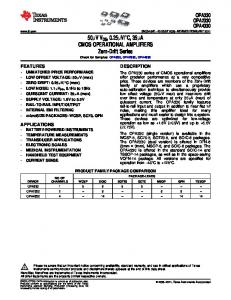
Figure 5. Input Characteristics Impedance of 3.3-V and 5-V Families BiCMOS Output Characteristics (ABT and LVT) Figure 6 is a simplified schematic of an ABT output stage. Data is transmitted to the gate of M1, which acts as a simple current switch. When M1 is turned on, current flows through R1 and M1 to the base of Q4, turning it on and driving the output low. At the same time, the base of Q2 is pulled low, turning off the upper output. For a low-to-high transition, the gate of M1 must be driven low, turning M1 off. Current through R1 will charge the base of Q2, pulling it high and turning on the Darlington pair, consisting of Q2 and Q3. Meanwhile, with its supply of base drive cut off, Q4 turns off, and the output switches from low to high. R2 is used to limit output current in the high state, and D1 is a blocking diode used to prevent reverse current flow in specific power-down applications. LVT I/Os have characteristics similar to ABT, with added CMOS pullup and pulldown for rail-to-rail switching.

6

VCC

ABT Output

D1 R1

R2

Q3 M1

VOUT Q4

ABT OUTPUT STAGE

Figure 6. Typical Output Cell for 5-V Families Figure 7 shows a simplified LVT output and illustrates the mixed-mode capability designed into the output stage. This combination of a high-drive TTL stage, along with the rail-to-rail CMOS switching, gives the LVT series exceptional application flexibility. These parts have the same drive characteristics as 5-V ABT devices and provide the dc drive needed for existing 5-V backplanes. Thus, using LVT is a simple way to reduce system power via the migration to 3.3-V operation. Not only can LVT devices operate as 3-V- to 5-V-level translators by supporting 5-V input or I/O voltages (VCC = 2.7 V to 3.6 V), but also the inputs can withstand 5.5 V, even when VCC = 0 V. This allows for the devices to be used under partial system power-down and live-insertion applications. VCC LVT Output D1 R2 LVC Output

VCC ALVC/LV Output

VCC

Q3 VOUT

VCC VOUT

Q4

5-V-TOLERANT OUTPUT STAGE (LVT/LVC)

VOUT

NON-5-V-TOLERANT OUTPUT STAGE (ALVC/LV)

Figure 7. Typical Output Cell for 3.3-V Families

7

CMOS Output Characteristics (ALVC, LVC, and LV) Figure 7 also shows a simplified LV, LVC, and ALVC output stage. LV and ALVC are pure 3.3-V families. They cannot be used to translate between 5-V and 3.3-V environments. ALVC is currently the fastest CMOS logic available. It is used primarily for high-speed memory and point-to-point applications with medium drive capability (±24 mA). LV is designed for low-speed, low-drive (±8–6 mA) applications. It is similar to HC and HCT. LVC, on the other hand, is used for on-board and memory applications that require medium performance and medium drive logic, as well as translation between 5-V and 3.3-V signals. These parts have the same drive characteristics as ALVC devices. Not only can LVC devices operate as 3-V- to 5-V-level translators by supporting 5.5-V input or I/O voltages (VCC = 3 V to 3.6 V), but the inputs can withstand 5.5 V, even when VCC = 0 V. This permits the devices to be used under partial system power-down and live-insertion applications. The IOH/VOH and IOL/VOL curves for the above familes are shown in Figures 8 and 9. With their specified IOL and IOH, some of these families will accommodate many standard bus specifications. However, these devices are capable of driving well beyond these limits. This is important when considering switching a low-impedance backplane on the incident wave. CBT, on the other hand, has no drive capability; its output impedance is purely resistive (V = I*R) as shown in Figures 2, 8, and 9. 3.3-V Families 4 TA = 25°C, VCC = 3.3 V, VIH = 3 V, VIL = 0 V

3.6 3.2

VOL – V

2.8

LV

2.4 2 1.6 LVC

1.2

ALVC

LVT2 0.8 LVT

0.4 0 0

10

20

30

40

50

60

70

80

90

100

IOL – mA

5-V Families 4 TA = 25°C, VCC = 5 V, VIH = 3 V, VIL = 0 V

3.6 3.2

VOL – V

2.8 2.4 2 1.6

ABT2

1.2 0.8

ABT

0.4 ABTE 0 0

10

20

30

40

50

60

70

80

90

100

IOL – mA

Figure 8. Output-Low Characteristic Impedance of 3.3-V and 5-V Families

8

3.3-V Families 3.2 2.8 2.4

TA = 25°C, VCC = 3.3 V, VIH = 3 V, VIL = 0 V

VOH – V

2 LVT2 1.6 LVC

LVT 1.2

LV

0.8

ALVC

0.4 0 –100

–90

–80

–70

–60

–50

–40

–30

–20

–10

0

–30

–20

–10

0

IOH – mA

5-V Families 4 3.6 3.2


ABTE

VOH – V

2.8 ABT

2.4 2 1.6 1.2

ABT2

0.8 0.4 0 –100

–90

–80

–70

–60

–50

–40

IOH – mA

Figure 9. Output-High Characteristic Impedance of 3.3-V and 5-V Families

Incident-Wave Switching Incident-wave switching ensures that, for a given transition (either high-to-low or low-to-high), the output reaches a valid VIH or VIL level on the initial wave front (i.e., does not require reflections). Figure 10 shows potential problems a designer might encounter when a device does not switch on the incident wave. A shelf below VIL(max), signal A, causes the propagation delay to slow by the amount of time it takes for the signal to reach the receiver and reflect back. Signal B shows the case where there is a shelf in the threshold region. When this happens, the input to the receiver is uncertain and could cause several problems associated with slow input edges, depending on the length of time the shelf remains in this region. Signal C will not cause a problem because the shelf does not occur until the necessary VIH level has been attained.

9

V

VIH(min) VIL(max)

A

B

C

Figure 10. Reflected-Wave Switching Using typical VOH and VOL values, along with data points from the curves, one can calculate the typical impedance the device can drive. For example, an ABT device can typically drive a line (from either end) in the 25-Ω range on the incident wave. However, if the same line is driven from the middle, the effective impedance seen by the driver is half its original value (12.5 Ω), which requires more current to switch it on the incident wave. For a low-to-high transition, (IOH = 85 mA @ VOH = 2.4 V): Z LH

+V

OH

*

(min) V OL(typ) I OH

+ 2.4 85V *mA0.3 V + 25 W

(1)

For a high-to-low transition, (IOL= 135 mA @ VOL= 0.5 V): Z HL

+V

OH

(typ)

*V I OL

OL

(max)

V * 0.5 V + 22 W + 3.5 135 mA

(2)

GTL and BTL Input/Output Structure BTL and GTL buffers are designed with minimal output capacitance (5-pF max), compared to a TTL output buffer (8-pF to 15-pF typ). A TTL or a CMOS output capacitance, coupled with the capacitance of the connectors, the traces, and the vias, reduces the characteristic impedance of the backplane. For a high-frequency environment, this phenomenon makes it difficult for the TTL or CMOS driver to switch the signal on the incident wave. A TTL or CMOS device needs a higher drive current than is presently available to be able to switch the signal under these conditions. However, increasing the output drive clearly increases the output capacitance. This scenario again reduces the characteristic impedance even more. That is why a lower-signal-swing family with reduced output capacitance, like BTL or GTL, is recommended when designing high-speed backplanes. The GTL input receiver is a differential comparator with one side connected to the reference voltage (VREF), which is provided externally (0.8-V typ). The threshold is designed with a precise window for maximum noise immunity (VIH = VREF + 50 mV and VIL = VREF – 50 mV). The output driver is an open-drain n-channel device that, when turned off, is pulled up to the output supply voltage (VTT = 1.2-V typ), and when turned on, the device can sink up to 40 mA of current (IOL) at a maximum output voltage (VOL) of 0.4 V. The output is designed for a doubly-terminated 50-Ω transmission line (25-Ω total load). The I/Os are designed to work independently of the device’s VCC. They can communicate with devices designed for 5-V, 3.3-V, or even 2.5-V VCC. The TTL input is a 5-V-tolerant, 3.3-V CMOS inverter (can interface with 5-V TTL signals). Bus hold is also provided on the TTL port to eliminate the need for external resistors when the I/Os are unused or floating. The TTL output is a bipolar output. It is similar to the LVT output structure. The family requires two power supplies to function: a 5-V supply [VCC(5)] for the GTL I/Os and 3.3-V supply [VCC(3.3)] for the LVTTL I/Os. The 5-V supply is used only on the GTL16612 and GTL16616. The maximum frequency at which the current family operates is 95 MHz (GTL16612 and GTL16616). Future functions such as GTL16622 and GTL16922, will be available as samples in early 1996 and will be released at the end of the year. They run as high as 200 MHz in both directions (GTL-to-TTL or TTL-to-GTL) and have a single 3.3-V power supply. GTL16922 has 5-V-tolerant TTL I/Os. Figure 11 shows a typical GTL input and output circuit and Figure 12 shows their characteristic impedance. Since GTL has an open-drain output, only the IOL/VOL curve is displayed.

10

GTL Input

GTL Output

VCC

VCC

BIAS Voltage

VREF

BIAS Voltage

VIN

VOUT

GTL B-PORT INPUT AND OUTPUT STAGE BTL/FB Input

VCC

BTL/FB Output

VCC VOUT

VIN

VREF

BTL/FB B-PORT INPUT AND OUTPUT STAGE

Figure 11. Typical GTL and BTL/FB Input and Output Cells

11

Input Characteristic Impedance 10 BTL/FB –10

I IN – mA

GTL –30

–50 TA = 25°C, VCC = 5 V, VIH = 3 V, VIL = 0 V

–70

–90 –1

0

1

2

3

4

5

6


Output Characteristic Impedance TA = 25°C, VCC = 5 V, VIH = 3 V, VIL = 0 V

2.8 2.4

VOL – V

2 1.6

1.47-V VIL (GTL/FB)

1.2

BTL/FB 0.85-V VIL (GTL)

0.8 GTL 0.4 0 0

25

50

75

100 125 150 175 200 225 250 275 300 IOL – mA

Figure 12. GTL and BTL/FB Input and Output Characteristic Impedance The BTL input receiver is a differential amplifier, with one side connected to an internal reference voltage. The threshold is designed with a narrow window (VIH = 1.62 V and VIL = 1.47 V). Unlike GTL, BTL requires a separate supply voltage for the threshold circuit. It eliminates any noise generated by the switching outputs. The output driver is an open-collector output with a termination resistor selected to match the bus impedance. When the device is turned off, the output is pulled up to output supply voltage (VTT = 2.1-V typ). The I/Os work independently of the device’s VCC; they communicate with devices designed for 5-V or 3.3-V VCC. The TTL input is a 5-V CMOS inverter and the output is a bipolar output similar to the ABT output structure. BTL requires three power supplies: the main power supply (VCC), the bias generator supply (BG VCC), and the bias supply voltage (BIAS VCC) that establishes a voltage between 1.62 V and 2.1 V on the BTL outputs when VCC is not connected. The recommended frequency at which the family runs is in the 30-MHz to 75-MHz range, depending on the application as well as the board layout. Figure 11 shows a typical BTL input and output circuit and Figure 12 shows their characteristic impedance. Since BTL has an open-collector output, only the IOL/VOL curve is displayed.

12

Power Consumption Several factors influence the power consumption of a device: frequency of operation, number of outputs switching, load capacitance, number of TTL-level inputs, junction temperature, ambient temperature, and thermal resistance of the device. The maximum operating frequency is limited by the thermal characteristics of the package. TI provides package power-dissipation information in data sheets under “absolute maximum ratings”. These numbers are calculated using a junction temperature of 150°C and a board trace length of 750 mils (no airflow). Refer to the Package Thermal Considerations application report in the ABT data book for the relationship between junction temperature and reliability. Traces, power planes, connectors, and cooling fans play an important role in improving the heat dissipation. Figures 13 through 15 show the typical power consumption with single- or all-outputs switching. Figure 16 also shows the maximum frequency at which a family can operate and still meet the VOH and VOL specifications. No frequency beyond the maximum number is acceptable. Note that all registered devices were tested based on the clock frequency, and the nonregistered devices were tested based on the input frequency.

13

Single-Output Switching Power Consumption 3.3-V Families 30 TA = 25°C, VCC = 3.3 V, VIH = 3 V, VIL = 0 V, No load


25

ALVC

20

LVC

LVT

15

LVT2 10

5 LV 0 0

10

20

30

40

50

60

70

80

90

100

Frequency – MHz

Single-Output Switching Power Consumption 5-V Families 80 TA = 25°C, VCC = 5 V, VIH = 5 V, VIL = 0 V, No load


70 60

ABT2

ABT

50 40

ABTE

30 20 10 CBT 0 0

10

20

30

40

50

60

70

Frequency – MHz

Figure 13. Power Consumption With Single-Output Switching

14

80

90

100

All-Outputs Switching Power Consumption 3.3-V Families 250 TA = 25°C, VCC = 3.3 V, VIH = 3 V, VIL = 0 V, No load

225


200 175

LVT2

LVT

LVC

150

ALVC

125 100

LV

75 50 25 0 0

10

20

40

50 60 Frequency – MHz

70

80

90

100

All-Outputs Switching Power Consumption 5-V Families

325

ABT

TA = 25°C, VCC = 5 V, VIH = 5 V, VIL = 0 V, No load

300 275 I CC – Supply Current – mA

30

250

ABT2

225 200 175 150 125

ABTE

100 75 50 25 CBT

0 0

10

20

30

40

50 60 Frequency – MHz

70

80

90

100

Figure 14. Power Consumption With All-Outputs Switching

15

All-Outputs Switching 325



300 275 I CC – Supply Current – mA


Single-Output Switching 150 140 130 120 110 100 90 80 70 60 50 40 30 20 10 0

GTL FB

250 225 200 175

FB

150 125 100

GTL

75 50 25 0

0

0

10 20 30 40 50 60 70 80 90 100

10 20 30 40 50 60 70 80 90 100 Frequency – MHz

Frequency – MHz

Figure 15. FB1650 and GTL16612 Power Consumption With Single- and All-Outputs Switching

5-V and 3.3-V Families 300

Frequency – MHz

250 200

TA = 25°C, VCC = 5 V (5-V families), VCC = 3.3 V (3.3-V families), VIH = 3 V, VIL = 0 V, Standard load

150 100 50 0 LV

LVC

LVT

LVT2

ALVC

ÍÍÍ ÂÂÂ ÍÍÍ ÂÂÂ ÍÍÍ ÂÂÂ ÈÈÈ ÎÎÎÁÁÍÍÍ ÂÂÂ ÍÍÍ ÂÂÂ ÈÈÈ ÎÎÎ ÁÁ ÂÂÂ ÈÈÈ ÎÎÎ ÁÁÍÍÍ ÍÍÍ ÂÂÂ ÈÈÈ ÎÎÎ ÁÁ ÍÍÍ ÂÂÂ ÈÈÈ ÎÎÎ ÁÁ ÂÂÂ ÈÈÈ ÎÎÎÁÁÍÍÍ ABT

ABT2

ABTE

GTL

FB

CBT†

† Data is based on the input signal characteristics: VIL = 0 V, VIH = 3 V, tr/tf = 2 ns.

Figure 16. Functional Frequency Using Standard Load Specified in Data Sheets

16

Power Calculation When calculating the total power consumption of a circuit, both the static and the dynamic currents must be taken into account. Both bipolar and BiCMOS devices have varying static-current levels, depending on the state of the output (ICCL, ICCH, or ICCZ), while a CMOS device has a single value for ICC. These values are given in the individual data sheets. All inputs or I/Os (except GTL or BTL I/Os), when driven at TTL levels, consume additional current because they may not be driven all the way to VCC or GND; therefore, the input transistors are not completely turned off. This value is known as ∆ICC and is provided in the data sheet. Dynamic power consumption results from charging and discharging both internal parasitic capacitances and external load capacitance. The parameter for CMOS devices that accounts for the parasitic capacitances is known as Cpd. It is obtained using equation 2 and is found in the data sheet. C pd

+ I V(dynamic) *C f CC

CC

(3)

L

i

Where: fi VCC CL ICC

= = = =

Input frequency (Hz) Supply voltage (V) Load capacitance (F) Measured value of current into the device (A)

Although a Cpd value is not provided for ABT and LVT, the ICC-versus-frequency curves display essentially the same information (see Figures 13 through 15). The slope of the curve provides a value in the form of mA /(MHz × bit) that, when multiplied by the number of outputs switching and the desired frequency, provides the dynamic power dissipated by the device without the load current. Equations 4 through 7 are used to calculate total power for CMOS or BiCMOS devices: PT

+P

S(tatic)

)P

(4)

D(ynamic)

CMOS CMOS-level inputs PS PD

+V + ǒC

CC

pd

I CC fi

)C

L

fo

Ǔ

(5)

V CC2

N sw

(6)

TTL-level inputs PS PD

+ [I ) (N + ǒC f ) C TTL

CC

pd

i

L

DICC

DC d)]

fo

V CC2

Ǔ

(7)

N sw

(8)

17

BiCMOS

ƪǒ

Note: ∆ICC = 0 for bipolar devices. PS

+V

PD

+ [DC

CC

DC en N H

en

N sw

I CCH NT V CC

)N fi

L

I CCL NT (V OH

Ǔ) *

*V

(1

OL

)

DC en)I CCZ

C L]

) (N

) [DC

en

TTL

DICC

DC d)

N sw

V CC

f2

ƫ

I CCD]

(9)

10 *3

(10)

Where: VCC = ICC = ICCL = ICCH = ICCZ = ∆ICC = DCen = DCd = NH = NL = Nsw = NT = NTTL=

Supply voltage (V) Power supply current (A) (from the data sheet) Power supply current (A) when outputs are in low state (from the data sheet) Power supply current (A) when outputs are in high state (from the data sheet) Power supply current (A) when outputs are in high-impedance state (from the data sheet) Power supply current (A) when one input is at a TTL level (from the data sheet) % duty cycle enabled (50% = 0.5) % duty cycle of the data (50% = 0.5) Number of outputs in high state Number of outputs in low state Total number of outputs switching Total number of outputs Number of inputs driven at TTL levels

fi = fo = f1 = f2 = VOH = VOL = CL = ICCD =

Input frequency (Hz) Ouput frequency (Hz) Operating frequency (Hz) Operating frequency (MHz) Output voltage (V) in high state Output voltage (V) in low state External load capacitance (F) Slope of the ICC-versus-frequency curve (mA/MHz × bit)

For GTL and BTL/FB devices, the power consumption/calculation is similar to a BiCMOS device, with the addition of the output power consumption through the pullup resistor, since GTL is open drain and BTL/FB is open collector.

Package Power Dissipation Thermal awareness became an industry concern when surface-mount technology (SMT) packages began replacing through-hole (DIP) packages in PCB designs. Circuits operating at the same power enclosed in a smaller package meant higher power density. To add to the issue, systems required increased throughput, which resulted in higher frequencies, increasing the power density even further. Not only do these same issues concern designers today, they are getting progressively more severe. Figure 17 explains part of the reason for increased attention to thermal issues. As a baseline for comparison, the 24-pin small-outline integrated circuit (SOIC) is shown, along with several fine-pitch packages supplied by TI, including the 24- and 48-pin SSOP, 24- and 48-pin TSSOP, and 100-pin thin quad flat pack (TQFP). The 24-pin TSSOP (8, 9, and 10 bits) allows for the same circuit functionality of the 24-pin SOIC to be packaged in less than a third of the area, while the 48-pin TSSOP (16, 18, and 20 bits) occupies less area and has twice the functionality of the 24-pin SOIC. This same phenomenon is expanded even further with the 100-pin TQFP (32 and 36 bits), which is the functional equivalent of four 24-pin or two 48-pin devices, with additional board savings over that of the SSOP packages. As the trend in packaging technology moves toward smaller packages, attention must be focused on the thermal issues that are created.

18

24-pin SOIC

Height = 2.65 mm Volume = 437 mm3 Lead pitch = 1.27 mm

24-pin SOIC Area = 165 mm2

24-pin SSOP

24-pin SSOP Area = 70 mm2

48-pin SSOP



100-pin SQFP

100-pin SQFP and 100-pin cavity TQFP Area = 266 mm2

48-pin TSSOP


48-pin TSSOP Area = 108 mm2

Height = 2 mm Volume = 140 mm3 Lead pitch = 0.65 mm


24-pin TSSOP



Figure 17. Advanced Packages A better understanding of the factors that contribute to junction temperature (TJ) provides a system designer with more flexibility when attempting to solve thermal issues. Device junction temperature is determined by equation 7: TJ

+ T ) (Q A

JA

P T)

(11)

Where: TJ TA ΘJA PT

= = = =

Junction (die) temperature (°C) Ambient temperature (°C) Thermal resistance of the package from the junction to the ambient (°C/W) Total power of the device (W)

Junction temperature is altered by lower chip power consumption, longer trace length, heatsinks, forced air flow, package mold compound, lead-frame size and material, surface area, and die size. Some of these are mechanically inherent in a particular package, while others are controlled by the designer and are application specific. Understanding which variables can be influenced by practicing good thermal-design techniques requires a more detailed investigation of power considerations as well as thermal-resistance measurements. The package power dissipation is calculated using a junction temperature (TJ) of 150°C and an ambient temperature (TA) of 55°C. ΘJA is calculated using a board trace length of 750 mils and no airflow. Table 2 provides the different ΘJA for different packages. Refer to the Package Thermal Considerations application report in the ABT data book for the relationship between junction temperature and reliability.

19

Table 2. ΘJA for Different Packages NO. OF PINS SOIC SSOP TSSOP QFP TQFP TQFP HP TQFP–HP

14

16

20

24

48

52

56

64

80

100

Package

D

D

DW

DW

––

––

––

––

––

––

ΘJA

76

73

59

56

––

––

––

––

––

––

Package

DB

DB

DB

DB

DL

ΘJA

185

175

164

152

80

68

Package

PW

PW

PW

PW

DGG

DGG

ΘJA

195

187

143

140

115

92

DL

Package

RC

PH

ΘJA

69

84

Package

PM

PN

ΘJA

96

89

PZ 79

Package

PCA

ΘJA

52.4

Advanced Packaging In addition to its strong commitment to provide fast, low-power, high-drive integrated circuits, TI is the clear-cut leader in logic packaging advancements. The development of the SSOP in 1989 provided system designers the opportunity to reduce the amount of board space required for bus-interface devices by 50 percent. Several 24-pin solutions, including the familiar SOIC, SSOP, and TSSOP are widely used, as well. The 48-/56-pin SSOP/TSSOP packages allow twice the functionality (16-, 18-, and 20-bit functions) in approximately the same or less board area as a standard SOIC. This is accomplished by using a 25-mil (0.635-mm) lead pitch, as opposed to 50 mil (1.27 mm) in SOIC. Figure 18 shows a typical pinout structure for the 48-pin SSOP/TSSOP. The flow-through architecture is standard for all Widebus devices, making signal routing easier during board layout. Also, note the distributed GND and VCC pins, which improve simultaneous switching performance, as discussed in the signal integrity section of this report.

20

8 Bit

16 Bit

8 Bit

1OE 1Y1 1Y2 GND 1Y3 1Y4 VCC 2Y1 2Y2 GND 2Y3 2Y4 3Y1 3Y2 GND 3Y3 3Y4 VCC 4Y1 4Y2 GND 4Y3 4Y4 4OE

1

48

2

47

3

46

4

45

5

44

6

43

7

42

8

41

9

40

10

39

11

38

12

37

13

36

14

35

15

34

16

33

17

32

18

31

19

30

20

29

21

28

22

27

23

26

24

25

2OE 1A1 1A2 GND 1A3 1A4 VCC 2A1 2A2 GND 2A3 2A4 3A1 3A2 GND 3A3 3A4 VCC 4A1 4A2 GND 4A3 4A4 3OE

Figure 18. Distributed Pinout of ’ABT16244A When using the small-pin-count SSOPs (8-, 9-, and 10-bit functions), the same functionality will occupy less than half the board area of an SOIC (70 mm2 vs 165 mm2). There is also a height improvement over the SOIC that is beneficial when the spacing between boards is a consideration. For very dense memory arrays, the packaging evolution has gone one step further with the TSSOP. The TSSOP thickness of 1.1 mm gives a 58-percent height improvement over the SOIC. Another packaging evolution is the EIAJ standard 100-pin TQFP package (0.5-mm lead pitch), which was developed for both the Widebus+ family (32-bit ABT) and the 18-bit FB+/ BTL universal bus transceivers (UBT). The FB version is a high-power package. A package cross-section, as shown in Figure 19, reveals a metal heatsink that facilitates the excellent thermal performance of the package.

ÌÌÌÌÌÌÌÌÌÌÌÌÌÌÌ ÎÎÎÎÎÎÎÎ ÏÏÏÏÏÏÏÏ ÌÌÌÌÌÌÌÌÌÌÌÌÌÌÌ ÎÎÎÎÎÎÎÎ ÏÏÏÏÏÏÏÏ ÏÏÏÏÏÏÏÏ Heatsink

Die

Figure 19. Cross-Section of Thermally Enhanced EIAJ 100-Pin TQFP For more information about the various packages used with the Advanced Bus-Interface families, refer to the Mechanical Data section in the ABT or LVT data book.

21

Output Capacitance TI designed both the CMOS and BiCMOS logic families for the lowest capacitance possible. GTL and BTL/FB, however, were designed to meet a 5-pF I/O capacitance on the B port. Figure 20 shows the typical input, I/O, and output capacitance of these families. Input Capacitance 15 13.5

Capacitance – pF

12 10.5 9

TA = 25°C, VCC = 5 V (5-V families), VCC = 3.3 V (3.3-V families), VIH = 3 V, VIL = 0 V, All unused inputs are biased low

9.5 6 4.5 3 1.5 0 LV

LVC

LVT

LVT2

ALVC

ÂÂÂ ÈÈÈ ÎÎÎÁÁÁ ÍÍÍ ÂÂÂ ÂÂÂ ÈÈÈ ÎÎÎ ÍÍÍ ÂÂÂ ÈÈÈ ÎÎÎÁÁÁ ÍÍÍ ABT

ABT2

ABTE

GTL

FB

CBT†

I/O Capacitance 15 TA = 25°C, VCC = 5 V (5-V families), VCC = 3.3 V (3.3-V families), VIH = 3 V, VIL = 0 V, All unused inputs are biased low

13.5

Capacitance – pF

12 10.5 9 9.5 6 4.5 3 1.5 0 LV

LVC

LVT

LVT2

ALVC

ÈÈÈ ÎÎÎ ÈÈÈ ÎÎÎ ÈÈÈ ÎÎÎ ÁÁÁ ÍÍÍ ÂÂÂ ÈÈÈ ÎÎÎ ÈÈÈ ÎÎÎ ÁÁÁ ÍÍÍ ÂÂÂ ÈÈÈ ÎÎÎ ÁÁÁ ÍÍÍ ÂÂÂ ÈÈÈ ÎÎÎÁÁÁ ÍÍÍ ÂÂÂ ABT

ABT2

ABTE

GTL


Figure 20. Capacitance Variation Between Families

22

FB

CBT†

ac Performance Simultaneous-Switching Phenomenon System designers are frequently concerned with the performance degradation of ICs when outputs are switched. TI’s priority, when designing the bus-interface families, is to minimize signal-integrity concerns and reduce the need for excess settling time of an output waveform. This section addresses the simultaneous switching performance of these families for both octals and Widebus devices. Figure 21 shows a simple model of an output pin, including the associated capacitance of the output load and the inherent inductance of the ground lead. The voltage drop across the GND inductor (VL) is determined by the value of the inductance and the rate of change in current across the inductor. When multiple outputs are switched from high to low, the transient current (di/dt) through the GND inductor generates a difference in potential on the chip ground with respect to the system ground. This induced GND variation can be observed indirectly, as shown in Figure 22. The voltage output low, peak or valley (VOLP, VOLV), is measured on one quiet output when all others are switched from high to low. Q

VO i

+ VL –

C

L

Figure 21. Simultaneous-Switching Output Model

VOHP

Volts – V

VOHV

VOLP 0 VOLV

0 t – Time – ns

Figure 22. Simultaneous-Switching-Noise Waveform

23

A similar phenomenon occurs with respect to the VCC plane on a low-to-high transition, known as voltage output high, peak or valley (VOHP, VOHV). Most problems are associated with a large VOLP because, in most cases, the range for a logic 0 is much less than the range for a logic 1 (see Figure 23). For a comprehensive discussion of simultaneous switching, see the Simultaneous Switching Evaluation and Testing application report or the Advanced CMOS Logic Designer’s Handbook from TI. The impact of these voltage noise spikes on a system can be extreme. The noise can cause loss of stored data, severe speed degradation, false clocking, and/or reduction in system noise immunity. For an overview of how propagation delay is affected by the switching of multiple outputs, please refer to the ac performance section of this report. Voltage VCC or VTT

Specified Output Voltage Range for Logic 1

Permissible Input Voltage Range for Logic 1

VOH Specified dc Noise Margin for Logic 1

Specified dc Noise Margin for Logic 0 Specified Output Voltage Range for Logic 0

VIH

VIL Permissible Input Voltage Range for Logic 0

VOL GND = 0

Output

Input Noise

Figure 23. dc Noise Margin Simultaneous-Switching Solutions IC manufacturers can reduce the effects of simultaneous switching by decreasing the inductance of the power pins, adding multiple power pins, and controlling the turn on of the output. These techniques are described in detail in the 1988 Texas Instruments Advanced CMOS Logic (ACL) Designer’s Handbook. Octal devices employ the standard end-pin GND and VCC configuration while maintaining acceptable simultaneous switching performance. Widebus series (16-, 18-, and 20-bit functions), on the other hand, are offered in an SSOP package (see the packaging section of this report) that was developed by TI to save valuable board space and reduce simultaneous switching effects. One might expect an increase in noise with 16 outputs switching in a single package; however, the simultaneous switching performance is actually improved. There is normally a GND pin for every two outputs and a VCC pin for every four outputs. This allows the transient current to be distributed across multiple power pins and decreases the overall current range of change (di/dt) effect. From basic circuit analysis, the induced voltage across an inductor is defined as: v

+ LǒdińdtǓ

Where: L = Inductance di/dt = Rate of change of the current

24

(12)

The current through an output is dependent on the voltage level and the load seen at the output. This can be expressed mathematically as: i

+ Cǒdv ńdtǓ

(13)

out

Analysis of equations 12 and 13 clearly shows that the more VCC and ground pins there are, the lower the lead inductance, resulting in less noise. As the speed of today’s circuits increases, di/dt increases and so does the generation of simultaneous-switching noise.The standard methodology devised by the industry to measure voltage bounce is to keep one output at either logic high (VOH) or logic low (VOL) and to switch all other outputs at a predefined frequency. Figures 24 through 26 show a comparison of the noise generation as (N – 1) outputs are switched simultaneously while the Nth output is held high or low. Refer to Figure 1 for the guaranteed VIL(max) and VIH(min) specification for various families. 3.3-V Families

5-V Families 1

1 TA = 25°C, VCC = 3.3 V, VIH = 3 V, VIL = 0 V, Standard load

0.9

0.8

0.8

0.7

0.7

0.6

0.6

VOLP – V

VOLP – V

0.9

0.5 0.4

0.5 0.4

0.3

0.3

0.2

0.2

0.1

0.1 0

0 LV†

LVC

LVT

LVT2

ALVC

TA = 25°C, VCC = 5 V, VIH = 3 V, VIL = 0 V, Standard load

ÈÈ ÈÈ ÈÈ ÈÈ ÈÈ ÈÈ ABT

ÂÂÂ ÂÂÂ ÂÂÂ ÎÎÂÂÂ ÎÎÂÂÂ ÎÎÂÂÂ ÎÎÂÂÂ ÎÎÂÂÂ ABT2

ABTE

CBT‡

† LV is tested using octal packages only. ‡ Data is based on the input signal characteristics: VIL = 0 V, VIH = 3 V, tr/tf = 2 ns.

Figure 24. Typical Output Low-Voltage Peak (VOLP) on 3.3-V and 5-V Families

3.3-V Families 3.5

3.5 3

TA = 25°C, VCC = 3.3 V, VIH = 3 V, VIL = 0 V, Standard load

3 2.5 VOHV – V

VOHV – V

2.5 2 1.5

2 1.5

1

1

0.5

0.5 0

0 LV†

LVC

LVT

LVT2

ALVC

ÈÈ ÈÈ ÈÈ ÈÈ ÈÈ ÈÈ ÈÈ ÈÈ ÈÈ ÈÈ

5-V Families

ÎÎÂÂÂ ÎÎÂÂÂ ÂÂÂ ÎÎÂÂÂ ÎÎÂÂÂ ÎÎÂÂÂ ÎÎÂÂÂ ÎÎÂÂÂ ÎÎÂÂÂ ÎÎ

TA = 25°C, VCC = 5 V, VIH = 3 V, VIL = 0 V, Standard load ABT

ABT2

ABTE

CBT‡

† LV is tested using octal packages only. ‡ Data is based on the input signal characteristics: VIL = 0 V, VIH = 3 V, tr/tf = 2 ns.

Figure 25. Typical Output High-Voltage Valley (VOHV) on 3.3-V and 5-V Families

25

GTL/BTL Output Voltage Peak

1.2

VOLP – V

1 0.8 0.6 0.4 0.2 0

ÏÏÏÏ ÏÏÏÏ ÏÏÏÏ ÏÏÏÏ ÏÏÏÏ ÏÏÏÏ ÍÍÍÍÏÏÏÏ ÏÏÏÏ ÍÍÍÍ ÍÍÍÍÏÏÏÏ GTL

BTL

2 1.8 1.6 1.4

0.75-V VIL (GTL)

VOHV – V

1.4

GTL/BTL Output Voltage Valley 1.47-V VIL (FB)

1.2 1 0.8 0.6 0.4 0.2 0

ÏÏÏÏ ÏÏÏÏ ÏÏÏÏ ÏÏÏÏ ÍÍÍÍÏÏÏÏ ÏÏÏÏ ÍÍÍÍ ÏÏÏÏ ÍÍÍÍ ÏÏÏÏ ÍÍÍÍ ÏÏÏÏ ÍÍÍÍ ÍÍÍÍÏÏÏÏ GTL

BTL

TA = 25°C, VCC = 5 V (BTL, GTL), VCC = 3.3 V (GTL), VIH = 3 V, VIL = 0 V, Standard load

Figure 26. Typical Output Voltage Peak (VOLP) and Valley (VOHV) on GTL and BTL

26

1.62-V VIH (FB)

0.85-V VIH (GTL)

Slew Rate Slew rate plays an important role in backplane or point-to-point application designs. The slower the output slew rate of a device, the less susceptible the signal is to reflections and noise. Based on this data, a designer knows how to terminate a bus or backplane. Using the characterization laboratory boards, the output slew rate (trise and tfall) was taken with and without the standard output load. Figures 27 and 28 show the output rise and fall times of each output taken between 10% and 90% for TTL, 0.5 V and 1 V for GTL, and 1.3 V and 1.8 V for BTL. Figures 29 and 30 show the rise and fall time as the number of outputs switching increases. The curves in both plots look almost flat between one output switching and all outputs switching. Rise Time 3.3-V and 5-V Families 2.4

TA = 25°C, VCC = 5 V (5-V families), VCC = 3.3 V (3.3-V families), VIH = 3 V, VIL = 0 V, All unused inputs are biased low, No load

2.2 2 Rise Time – ns

1.8 1.6 1.4 1.2 3.3-V Families

1 0.6 0.4 0.2 0 LV

LVC

LVT

LVT2

ÁÁ ÈÈÎÎÁÁÍÍÂÂ ÈÈÎÎÁÁÍÍÂÂ ÈÈÎÎÁÁÍÍÂÂ ÈÈÎÎÁÁÍÍ 5-V Families

0.8

ALVC

ABT

ABT2

ABTE

GTL

FB

CBT†

Fall Time 3.3-V and 5-V Families 2.4

TA = 25°C, VCC = 5 V (5-V families), VCC = 3.3 V (3.3-V families), VIH = 3 V, VIL = 0 V, All unused inputs are biased low, no load

2.2 2

Fall Time – ns

1.8 1.6 1.4 1.2 1

3.3-V Families

5-V Families

0.8 0.6 0.4 0.2 0 LV

LVC

LVT

LVT2

ALVC

ÎÎ ÁÁ ÍÍ ÈÈÎÎÁÁÍÍÂÂ ÈÈÎÎÁÁÍÍÂÂ ABT

ABT2

ABTE

GTL

FB

CBT†


Figure 27. Typical Output Rise and Fall Time Measured Between Specified Levels or Voltages

27

Rise Time 3.3-V and 5-V Families 3.3 3 2.7 Rise Time – ns

2.4 2.1 1.8 1.5 1.2 0.9 0.6 0.3 0 LV

LVC

LVT

ÁÁÁ ÁÁÁ ÁÁÁ ÎÎÁÁÁ ÂÂÂ ÁÁÁ ÎÎ ÈÈÎÎÁÁÁ ÂÂÂ ÍÍÍ ÂÂÂ ÈÈÎÎÁÁÁ ÂÂÂ ÍÍÍ ÈÈÎÎÁÁÁ ÂÂÂ ÍÍÍ ÈÈÎÎÁÁÁ ÂÂÂ ÍÍÍ ÈÈÎÎÁÁÁ ÂÂÂ ÍÍÍ ÈÈÎÎÁÁÁ

TA = 25°C, VCC = 5 V (5-V families), VCC = 3.3 V (3.3-V families), VIH = 3 V, VIL = 0 V, All unused inputs are biased low, Standard load

3.3-V Families

LVT2

ALVC

ABT

5-V Families

ABT2

ABTE

GTL

FB

CBT†

Fall Time 3.3-V and 5-V Families 3.3 3 2.7 Fall Time – ns

2.4 2.1

3.3-V Families

TA = 25°C, VCC = 5 V (5-V families), VCC = 3.3 V (3.3-V families), VIH = 3 V, VIL = 0 V, All unused inputs are biased low, Standard load

1.8 1.5 1.2 0.9 0.6 0.3 0 LV

LVC

LVT

LVT2

ALVC

ÁÁÁ ÎÎÁÁÁ ÁÁÁ ÎÎ ÈÈÎÎÁÁÁ ÍÍÍ ÂÂÂ ÈÈÎÎÁÁÁ ÍÍÍ ÂÂÂ ÍÍÍ ÂÂÂ ÈÈÎÎÁÁÁ ABT

ABT2

5-V Families

ABTE

GTL

FB

CBT†


Figure 28. Typical Output Rise and Fall Time Measured Between Specified Levels or Voltages

28

Rise Time vs No. of Outputs Switching 3.3-V Families 5.5

Rise Time – ns

4.5

TA = 25°C, VCC = 3.3 V, VIH = 3 V, VIL = 0 V, Frequency = 10 MHz, Standard load

LV

3.5

ALVC 2.5

LVT2 LVC LVT

1.5 0

2

4

6

8

10

12

14

16

No. of Outputs Switching

Rise Time vs No. of Outputs Switching 5-V Families ABTE CBT† 2.5 ABT

Rise Time – ns

ABT2

FB TA = 25°C, VCC = 5 V, VIH = 3 V, VIL = 0 V, Frequency = 10 MHz, Standard load

1.5

GTL

0.5 0

2

4

6

8

10

12

14

16

No. of Outputs Switching † Data is based on the input signal characteristics: VIL = 0 V, VIH = 3 V, tr/tf = 2 ns.

Figure 29. Typical Output Rise Time as the Number of Outputs Switching Increases

29

Fall Time vs No. of Outputs Switching 3.3-V Families TA = 25°C, VCC = 3.3 V, VIH = 3 V, VIL = 0 V, Frequency = 10 MHz, Standard load

4

Fall Time – ns

LV

3 LVT2 LVC ALVC 2

LVT 1 0

2

4

6

8

10

12

14

16

No. of Outputs Switching

Fall Time vs No. of Outputs Switching 5-V Families

Fall Time – ns

2.5

TA = 25°C, VCC = 5 V, VIH = 3 V, VIL = 0 V, Frequency = 10 MHz, Standard load

CBT†

ABTE FB ABT

1.5

ABT2

GTL 0.5 0

2

4

6

8 10 No. of Outputs Switching

12

14


Figure 30. Typical Output Fall Time as the Number of Outputs Switching Increases

30

16

Effects of Simultaneous Switching and Capacitive Loading on Propagation Delay Another factor that may be of concern to a designer is the change in propagation delay when more outputs are switching or when the output capacitive load is varying. This data is very useful, since a typical application would use all outputs simultaneously. In addition, it usually requires different loading conditions than the data sheet specifies. Data sheets do not show the performance of the device with different loads; they only use the standard load specified in data sheets. Figure 31 shows the propagation delay of a device as the number of outputs switching increases. Figures 32 and 33 show the increase in propagation delays (tPHL and tPLH) as the output capacitive load increases from 0 pF to 200 pF.

31

Propagation Delay Time vs No. of Outputs Switching 3.3-V Families 9 TA = 25°C, VCC = 3.3 V, VIH = 3 V, VIL = 0 V, Frequency = 10 MHz, Standard load

LV

Propagation Delay – ns

8

7

6

5

4

LVC LVT2 LVT

3

ALVC 2 0

2

4

6


12

14

16

Propagation Delay Time vs No. of Outputs Switching 5-V Families FB


4

ABT

3 ABT2 GTL ABTE

TA = 25°C, VCC = 5 V, VIH = 3 V, VIL = 0 V, Frequency = 10 MHz, Standard load

2

1

CBT† 0 0

2

4

6


12

14


Figure 31. Typical Propagation Delay vs Number of Outputs Switching (Standard Load)

32

16

Typical tPHL vs Capacitive Load 3.3-V Families 12 TA = 25°C, VCC = 3.3 V, VIH = 3 V, VIL = 0 V, Frequency = 10 MHz


10

8 LV 6

4

LVT

LVC LVT2

2 ALVC 0 0

50

100

150

200

Capacitive Load – pF

Typical tPHL vs Capacitive Load 5-V Families 7 TA = 25°C, VCC = 5 V, VIH = 3 V, VIL = 0 V, Frequency = 10 MHz


6

ABT2 ABTE

5 GTL 4 FB

ABT

3

2

1 CBT† 0 0

50

100

150

200

Capacitive Load – pF † Data is based on the input signal characteristics: VIL = 0 V, VIH = 3 V, tr/tf = 2 ns.

Figure 32. Typical tPHL vs Capacitive Load

33

Typical tPLH vs Capacitive Load 3.3-V Families 12 TA = 25°C, VCC = 3.3 V, VIH = 3 V, VIL = 0 V, Frequency = 10 MHz


10

8 LV 6

LVT

4 LVT2 LVC 2 ALVC 0 0

50

100

150

200

Capacitive Load – pF

Typical tPLH vs Capacitive Load 5-V Families 7 TA = 25°C, VCC = 5 V, VIH = 3 V, VIL = 0 V, Frequency = 10 MHz


6

5 ABT2 4 GTL 3

ABT

FB ABTE

2

1 CBT† 0 0

50

100 Capacitive Load – pF


Figure 33. Typical tPLH vs Capacitive Load

34

150

200

Skew Skew is a term that is used to define the difference in time between two different signal edges. There are several different types of skew currently being used; however, the skew discussed here is the skew of propagation delays across the outputs of a device. More specifically, it is the difference between the largest value obtained for a propagation delay and the smallest value across all of the outputs. For example, if output 3 has the largest propagation delay (tPLH) and output 14 has the smallest, the output skew for this device would be the difference between the propagation delays for output 3 and output 14 (see Figure 34).

1 tPLH14 2

3

• • •

tPLH3

16

Figure 34. Skew = |tPLH3 – tPLH4| The data presented in this report is taken from devices that have one output switching at a time (VCC = MIN and TA = 85°C). This data represents the average worst-case condition skew. Figure 35 shows the skew of the different families using the standard load specified in data sheets. Skew Data 3.3-V Families and 5-V Families 1 TA = 85°C, VCC = 4.5 V (5-V families), VCC = 3 V (3.3-V families), VIH = 3 V, VIL = 0 V, Standard load

0.9 0.8

Skew – ns

0.7 0.6

3.3-V Families

5-V Families

0.5 0.4 0.3 0.2 0.1 0 LV

LVC

LVT

LVT2

ALVC

ÈÈÈÎÎ ÍÍÂÂ ÈÈÈÎÎÁÁÍÍÂÂ ÈÈÈ ÂÂ ÈÈÈÎÎÁÁÍÍÂÂ ABT

ABT2

ABTE

GTL

FB

CBT†


Figure 35. Typical Skew Between Outputs

35

Bus-Hold Circuit The most effective method to provide defined levels for a floating bus is to use TI’s bus hold as a built-in feature on selected families (see Table 3). Table 3. List of Devices With Bus Hold FAMILY

BUS HOLD

ABT WIdebus+ (32- and 36-bit)

All devices

ABT Octals and Widebus

Selected devices

Low Voltage (LVT and ALVC)

All devices

LVC Octals and Widebus

Selected devices

GTL

A port only

Bus hold is a circuit used in TI’s selected families to help solve the floating-input problem and eliminate the need for pullup and pulldown resistors. It consists of two back-to-back inverters, with the output fed back to the input via a resistor (see Figure 36). To understand how the bus-hold cell operates, let’s assume that an active driver has switched the line to a high level. This results in no current flowing through the feedback circuit. Now, the driver goes in the high-impedance state and the bus-hold circuit holds the high level via the feedback resistor. The current requirement of the bus hold is determined only by the leakage current of the circuit. The same condition applies when the bus is in the low state and then goes inactive.

Input

Figure 36. Typical Bus-Hold Cell Table 4 shows the data-sheet dc specifications for bus hold. The first specification is the minimum available current to hold the bus at 0.8 V or 2 V. These voltages are the guaranteed low and high levels for TTL inputs. The second specification is the maximum current that the bus hold sources or sinks at any input voltage between 0 V and 3.6 V (for low-voltage families) or between 0 V and 5.5 V (for ABT). The bus-hold current becomes minimal as the input approaches the rails. The output leakage currents, IOZH and IOZL, are insignificant for transceivers with bus hold since a true leakage test cannot be achieved due to the existence of the bus-hold circuit. Since bus hold behaves as a small driver, it tends to source or sink a current that is opposite in direction to the leakage current. This situation is true for transceivers with bus hold only and does not apply to buffers. Note that all LVT, ABT Widebus+, selected ABT and LVC octals, and Widebus devices have the bus-hold feature. Refer to Table 4 or the manufacturer for more information. Table 4. Data-Sheet Specification for Bus Hold

electrical characteristics over recommended operating free-air temperature range (for families with bus-hold features) PARAMETER II(hold) ( )

TEST CONDITIONS LVT, LVC, ALVC

Data inputs or I/Os

VCC = 3 V VCC = 3.6 V,

II(hold) ( )

Widebus+ ABT Widebus+ and selected ABT Widebus ABT

IOZH/IOZL LVT, LVC, ALVC IOZH/IOZL

36

ABT LVT, LVC, ALVC

Data inputs or I/Os

5V VCC = 4 4.5 VCC = 5.5 V,

MIN VI = 0.8 V VI = 2 V VI = 0 to 3.6 V VI = 0.8 V VI = 2 V VI = 0 to 5.5 V

MAX

UNIT

75 µA

–75 ±500 100

µA

–100 ±500

Transceivers with bus hold

This test is not a true IOZ test since bus hold is always y active on an I/O pin. It tends to supplyy a current that is opposite in direction to the output leakage current.

±1

Buffers with bus hold

This test is a true IOZ test since bus hold does not exist on an output pin.

±10

µA ±1

±5

µA

Partial Power Down Partial power down and live insertion are becoming a major issue in today’s system designs. Many new standards have included this as part of their specification. The plug-and-play feature is beginning to dominate the PC market and the telecom industry has been using it for a long time. When a system is partially down, the unpowered device is expected to go into a high-impedance state so the device does not disturb or disrupt the data on the bus. When using standard CMOS devices, there is a path from either the input or the output (or both) to VCC. This prevents partial power down for such applications as hot-card insertion without adding current-limiting components. This is not the case with ABT, LVT, LVC, GTL, and BTL, as these paths have been eliminated with the use of either blocking diodes or current-blocking circuitries. Figure 37 shows functionally-equivalent schematics of the input and output structures for these families. Refer to Figures 5 and 10 for more detail on the input and output behavior under these conditions. Consider the situation shown in Figure 38. The driving device is powered with VCC = 5 V while the receiving device is powered down (VCC = 0). If these devices are either LV, ALVC, or ALB, the receiver can be powered up through the diode, D2 and D3, when the driver is in a high state. ABT, LVT, LVC, GTL, and BTL devices do not have a comparable path and are thus immune to this problem, making them more desirable for this application. The electrical characteristics table in the data sheet has a specification called Ioff. This specification shows the test condition and the maximum leakage a device can source or sink when VCC is off. Refer to the individual data sheets for more details. LV and ALB Only VCC

VCC

D2

•••

Input D1

Output

•••

Input

D4

D5

a) ALVC, LV, AND ALB EQUIVALENT I/O STRUCTURE

Output D6

b) ABT, LVT, LVC, GTL, AND BTL EQUIVALENT I/O STRUCTURE

Figure 37. Simplified Input Structures for CMOS and ABT Devices

VCC = 5 V

VCC = 0

Figure 38. Example of Partial-System Power Down

37

Power-Up or Power-Down High Impedance Power-up 3-state circuitry is another feature that TI offers on selected LVT, ABT, and FB. This feature keeps the output in a high-impedance state during power up or power down, regardless of the output-enable control pin’s state (VCC = 0 V to 2.1 V for ABT and FB, and VCC = 0 V to 1.5 V for LVT). After VCC reaches the specified value, the output-enable control takes over and puts the device in the required state (see Figure 39). The electrical characteristics table in the data sheet has both the power-up and power-down specifications (IOZPU and IOZPD). These specifications show the test condition and the maximum leakage an output can source or sink when VCC is between 0 V and 2.1 V for ABT and FB or between 0 V and 1.5 V for LVT (the nomenclature for the selected LVT devices that offer this feature is LVTZ). Refer to the LVT data book for more details. Power-up or power-down high impedance can also be achieved with other families by adding an external pullup or pulldown resistor (typically 1 kΩ) from the output-enable pin to VCC (active-low devices) or to GND (active-high devices) (see Figure 40). This ensures the high-impedance state during the full VCC ramp. As long as the output-enable pin is not driven to an active state by the controlling device, an ASIC, FPGA, or PAL, the output remains disabled. 5

4

3

2.1 V

2

2.1 V

1.5 V

1.5 V

1

0 Off

ABT, FB

LVTZ

On

Off

Off

On

Off

Output Status

Figure 39. Power-Up and Power-Down High Impedance Up to 2.1 V (ABT, FB) and 1.5 V (LVTZ)

ASIC, FPGA, or PAL Device VCC

VCC IR†

Control Circuit

Enable Pin (active low) IOL†

† IOL > IR, so the control signal can override the pullup resistor.

Figure 40. Power-Up High Impedance With Active-Low Control Pin

38

ABTE, FB, and CBT (CBT6800 only) have an added feature called BIAS VCC. This feature is used to precharge the output, trace, and connector capacitance during power up. This circuit prevents the device from spiking the backplane and disrupting the data during hot-card insertion. For this feature to work, both ground and BIAS VCC pins must make contact before VCC does (both pins should be the longest on the card).

Additional Design Considerations for GTL and BTL/FB GTL To successfully design with the GTL family, several rules and techniques with regard to voltage generation and proper termination must be followed. First, both 3.3-V and 5 V-VCC are needed in the current generation of GTL devices (only the 3.3-V VCC will be needed in the next-generation GTL). Second, the termination voltage (VTT = 1.2 V) should be regulated from the 5-V- VCC, keeping in mind the current requirements of the outputs (40 mA per output). There are several linear regulators that are capable of performing this function. Depending on the design, the regulator could be either on the backplane itself or on the individual cards. Third, the reference voltage (VREF = 0.8 V) must be generated from VTT. The VREF voltage can be generated using a simple voltage-divider circuit with an appropriate bypass capacitor (0.01 µF or 0.1 µF) placed as close as possible to the VREF pin. The VREF input circuitry consumes very little power (1-µA max). This enables several devices to have their VREF pin connected to the same voltage-divider circuit, thus eliminating the need for multiple voltage-divider circuits (see Figure 41). VTT

R VREF 2R

C

Figure 41. Proposed Circuit to Generate VREF BTL/FB For the BTL family, there are four power supplies and two grounds to be connected. For live-insertion applications, the power-up scheme should be as follows: the GND lead should make contact first, followed by BIAS VCC. This sequence precharges the board and the device capacitance and establishes a voltage between 1.62 V and 2.1 V on the BTL outputs. Next, VCC makes contact and, as it ramps up, the BIAS-VCC circuitry starts to turn off. When VCC reaches its final value, the BIAS VCC circuitry is completely isolated and does not interfere with the device functionality. BG-VCC and BG-GND pins are used to supply power to the bias-generator input circuitry. Both signals must be isolated from the rest of the power supplies. This ensures the signal integrity at the BTL input. The 2.1-V VTT should be regulated from a higher voltage and should supply enough current to switch all 18 outputs (100 mA per output). VTT variation should not exceed ±2% and it is recommended that proper bypass capacitors (0.01 µF or 0.1 µF) be used. The termination resistor should not exceed ±1% of its resistance value.

39

Conclusion Today’s high-speed bus and point-to-point applications require devices that can provide high performance, excellent signal integrity, and cost effectiveness. TI’s Advanced System Logic (ASL) group offers the widest selection of logic families that meet these requirements, from low drive (6 mA) to high drive (180 mA) and from low performance (16 ns) to high performance (sub 2 ns) propagation delay. These families are leading the industry and are used extensively in almost every application (PCs, workstations, telecom, networking, etc.). ASL also offers a wide variety of packaging options, including advanced packaging such as the plastic TQFP, SSOP, and TSSOP. The product offerings, coupled with the information provided in this application report, enable the designer to have a complete understanding of these products and their behavior. Table 5 summarizes the various circuit features and characteristics that were discussed in this application report. It can be used as a reference guide to help select the appropriate device for any application. Table 5. Summary of the Various Features and Characteristics of the Device Families

∆t /∆† (ns/V)

Drive IOL/ IOH (mA)

ICCD (mA/ MHz Bit)

TYP VOLP/ VOHV (V)

TYP Output Rise/ Fall (ns)

TYP tPD vs Cap. (ns/ pF)

TYP tPD vs SS (ns/ Nsw)

MAX tPD (ns)

TYP Skew (ns)

MAX ICC CMOS (mA)

LV

100

8/–8†

0.22

0.70/ 2.4

1.81/ 2.44

0.028

0.11

16

0.74

0.02

LVC

10

24/–24

0.23

0.57/ 2.4

0.54/ 0.6

0.014

0.04

5.2

0.27

0.02

LVT

10

64/–32

0.12

0.38/ 2.47

0.47/ 0.49

0.01

0.04

4.1

0.48

LVTZ

10

64/–32

0.12

0.38/ 2.47

0.47/ 0.49

0.01

0.04

4.1

LVT2

10

12/–12

0.12

0.34/ 2.6

0.5/ 0.5

0.018

0.05

ALVC

10

24/–24

0.27

0.70/ 2.38

0.33/ 0.29

0.014

ABT

10

64/–32

0.49

0.54/ 3.3

0.52/ 0.42

ABT2

10

12/–12†

0.49

0.40/ 3.3

ABTE

10

90/–60

0.42

GTL

10

40§

FB

5

CBT

–

5-V Tol.

PU3S

Bus Hold

25-Ω Output Series Resistor

TYP Control/ I/O Cap. (pF) 2.5/ 2.5/7

√‡

0.12/ 5/ 0.12†

√

√

3.5/ 4/10

0.48

0.12/ 5/ 0.12†

√

√

3.5/ 4/8

4.9

0.35

0.12/ 5/ 0.12†

√

0.05

3.4

0.45

0.013

0.04

4.2

0.25

2/ 30/ 2†

√‡

√‡

0.62/ 0.55

0.019

0.04

4.2

0.18

2/ 30/ 2†

√‡

√‡

0.70/ 3.1

0.75/ 0.47

0.024

0.04

5.2

0.11

36/ 48/ 32

0.30

0.40/ 1.1

0.64/ 0.56

0.0054

0.04

4

0.17

120

100§

0.20

1.3/ 1.9

0.43/ 0.37

0.014

0.04

5.6

0.30

60†

0/0

0

0.14/ 2.89

0.64/ 0.56

0.013

0.02

0.25

0.23

√

0.04

0.003†

√ √

√‡

3.3/ 5.5/9

√†

† Unless otherwise noted in data sheets ‡ Selected devices only § Open-drain/open-collector devices

40

MAX ICCH/ ICCL/ ICCZ BiCMOS (mA)

√

√

3.5/ 4/10

√

√‡

3.5/ 6/7.5 3/ 3/6

√

3/ 3/6

√

2.5/ 2.5/4.5

√

3.5/ 3.5/4 5/ 5/4 3/ 6/6

Acknowledgment The author of this document is Ramzi Ammar.

References 1 Texas Instruments Advanced BiCMOS Data Book 1994, SCBD002B. 2 Gunning, Bill; Yuan, Leo; Nguyen, Trung; Wong, Tony, GTL: “A Low-Voltage Swing Transmission-Line Transceiver”, March 15, 1991. 3 Texas Instruments, “Package Thermal Considerations”, Advanced BiCMOS Data Book 1994, SCBD002B, page 13-97.

41

Understanding Advanced Bus-Interface ... - Texas Instruments

Understanding Advanced Bus-Interface ... - Texas Instruments

Suggest Documents

Understanding Buffered and Unbuffered ... - Texas Instruments

Understanding and Interpreting Standard-Logic ... - Texas Instruments

TL431 datasheet - Texas Instruments

INA121 - Texas Instruments

LMP7721 - Texas Instruments

APPLICATION BULLETIN - Texas Instruments

DSD1794A - Texas Instruments

Datasheet - Texas Instruments

Drv8825 - Texas Instruments

LM4041 datasheet - Texas Instruments

Drv8825 - Texas Instruments

AFE5809 - Texas Instruments

TMP102 - Texas Instruments

ADS1115 - Texas Instruments

OPT101 - Texas Instruments

LMT86(-Q1) - Texas Instruments

OPA121 - Texas Instruments

Data Sheet - Texas Instruments

CC2520 - Texas Instruments

SBOS432E - Texas Instruments

MicroSiP - Texas Instruments

LM317 - Texas Instruments

LM2576 - Texas Instruments

Datasheet - Texas Instruments