Understanding and Abstracting Total Data Center Power Steven Pelley† David Meisner† Thomas F. Wenisch† James W. VanGilder‡ {spelley, meisner, twenisch}@umich.edu
[email protected] †
ABSTRACT The alarming growth of data center power consumption has led to a surge in research activity on data center energy efficiency. Though myriad, most existing energy-efficiency efforts focus narrowly on a single data center subsystem. Sophisticated power management increases dynamic power ranges and can lead to complex interactions among IT, power, and cooling systems. However, reasoning about total data center power is difficult because of the diversity and complexity of this infrastructure. In this paper, we develop an analytic framework for modeling total data center power. We collect power models from a variety of sources for each critical data center component. These component-wise models are suitable for integration into a detailed data center simulator that tracks subsystem utilization and interaction at fine granularity. We outline the design for such a simulator. Furthermore, to provide insight into average data center behavior and enable rapid back-of-theenvelope reasoning, we develop abstract models that replace key simulation steps with simple parametric models. To our knowledge, our effort is the first attempt at a comprehensive framework for modeling total data center power.
1.
‡
Advanced Computer Architecture Lab The University of Michigan
INTRODUCTION
Data center power consumption continues to grow at an alarming pace; it is projected to reach 100 billion kWh at an annual cost of $7.4 billion within two years [18], with a world-wide carbon-emissions impact similar to that of the entire Czech Republic [9]. In light of this trend, computer systems researchers, application designers, power and cooling engineers, and governmental bodies have all launched research efforts to improve data center energy efficiency. These myriad efforts span numerous aspects of data center design (server architecture [8, 10], scheduling [11, 13], power delivery systems [5], cooling infrastructure [14], etc.). However, with few exceptions, existing efforts focus narrowly on energy-efficiency of single subsystems, without considering global interactions or implications across data center subsystems. As sophisticated power management features proliferate, the dynamic range of data center power draw (as a function of utilization) is increasing, and interactions among power management strategies across subsystems grow more complex; subsystems can no longer be analyzed in isolation. Even questions that appear simple on their face can become quite complicated. Reasoning about total data center power is difficult because of the diversity and complexity of data center infrastructure. Five distinct sub-systems (designed and marketed by different industry segments) account for most of a data center’s power draw: (1) servers and storage systems, (2) power conditioning equipment, (3) cooling and humidification systems, (4) networking equipment, and (5) lighting/physical security. Numerous sources have reported power breakdowns [18, 10]; Table 1 illustrates a typical breakdown today. The first three subsystems dominate and their power draw can vary drastically with data center utilization. Cooling power further depends on ambient weather conditions around the data center facility. Even the distribution of load in each subsystem can
APC by Schneider Electric
Table 1: Typical Data Center Power Breakdown. Servers Cooling Power Cond. Network Lighting 56%
30%
8%
5%
1%
affect power draws, as the interactions among sub-systems are non-linear In this paper, our objective is to provide tools to the computer systems community to assess and reason about total data center power. Our approach is two-fold, targeting both data center simulation and abstract analytic modeling. First, we have collected a set of detailed power models (from academic sources, industrial white papers, and product data sheets) for each critical component of data center infrastructure, which describe power draw as a function of environmental and load parameters. Each model describes the power characteristics of a single device (i.e., one server or computer room air handler (CRAH)) and, as such, is suitable for integration into a detailed data center simulator. We describe how these models interact (i.e., how utilization, power, and heat flow among components) and outline the design of such a simulator. To our knowledge, we are the first to describe an integrated data center simulation infrastructure; its implementation is underway. Although these detailed models enable data center simulation, they do not allow direct analytic reasoning about total data center power. Individual components’ power draw vary non-linearly with localized conditions (i.e., temperature at a CRAH inlet, utilization of an individual server), that require detailed simulation to assess precisely. Hence, to enable backof-the-envelope reasoning, we develop an abstract model that replaces key steps of the data center simulation process with simple parametric models that enable analysis of average behavior. In particular, we abstract away time-varying scheduling/load distribution across servers and detailed tracking of the thermodynamics of data center airflow. Our abstract model provides insight into how data center sub-systems interact and allows quick comparison of energy-efficiency optimizations.
2.
RELATED WORK
The literature on computer system power management is vast; a recent survey appears in [7]. A tutorial on data center infrastructure and related research issues is available in [1]. Numerous academic studies and industrial whitepapers describe or apply models of power draw for individual data center subsystems. Prior modeling efforts indicate that server power varies roughly linearly in CPU utilization [5, 16]. Losses in power conditioning systems and the impact of power overprovisioning are described in [5, 15]. Our prior work proposes mechanisms to eliminate idle power waste in servers [10]. Other studies have focused on understanding the thermal implications of data center design [6, 14]. Power- and coolingaware scheduling and load balancing can mitigate data center cooling costs [11, 13]. Though each of these studies examines particular aspects of data center design, none of these present a comprehensive model for total data center power draw.
Server Racks
CRAH Cooling Tower
...
...
PDU
UPS Server Racks
Pump
CRAH
13.2kV
115kV
Transformer
Pump Water PDU
208 V
Chiller
Air Electric
1kV
Figure 1: Power and Cooling Flow.
3.
DATA CENTER POWER FLOW
We begin by briefly surveying major data center subsystems and their interactions. Figure 1 illustrates the primary powerconsuming subsystems and how power and heat flow among them. Servers (arranged in racks) consume the dominant fraction of data center power, and their power draw varies with utilization. The data center’s power conditioning infrastructure typically accepts high-voltage AC power from the utility provider, transforms its voltage, and supplies power to uninterruptible power supplies (UPSs). The UPSs typically charge continuously and supply power in the brief gap until generators can start during a utility failure. From the UPS, electricity is distributed at high voltage (480V-1kV) to power distribution units (PDUs), which regulate voltage to match IT equipment requirements. Both PDUs and UPSs impose substantial power overheads, and their overheads grow with load. Nearly all power dissipated in a data center is converted to heat, which must be evacuated from the facility. Removing this heat while maintaining humidity and air quality requires an extensive cooling infrastructure. Cooling begins with the computer room air handler (CRAH), which transfer heat from servers’ hot exhaust to a chilled water/glycol cooling loop while supplying cold air throughout the data center. CRAHs appear in various forms, from room air conditioners that pump air through underfloor plenums to in-row units located in containment systems. The water/glycol heated by the CRAHs is then pumped to a chiller plant where heat is exchanged between the inner water loop and a second loop connected to a cooling tower, where heat is released to the outside atmosphere. Extracting heat in this manner requires substantial energy; chiller power dominates overall cooling system power, and its requirements grow with both the data center thermal load and outside air temperature.
4.
MODELING DATA CENTER POWER
Our objective is to model total data center power at two granularities: for detailed simulation and for abstract analysis. Two external factors primarily affect data center power usage: the aggregate load presented to the compute infrastructure and the ambient outside air temperature (outside humidity secondarily affects cooling power as well, but, to limit model complexity, we do not consider it here). We construct our modeling framework by composing models for the individual data center components. In our abstract models, we replace key steps that determine the detailed distribution of compute load and heat with simple parametric models that enable reasoning about average behavior.
U u κ ` E π f
Table 2: Variable Definitions. Data Center Utilization T Temperature Component Utilization m ˙ Flow Rate Containment Index Cp Heat Capacity Load Balancing Coefficient NSrv # of Servers Heat Transfer Effectiveness P Power Loss Coefficient q Heat Fractional Flow Rate
Framework. We formulate total data center power draw, PTotal , as a function of total utilization, U , and ambient outside temperature, TOutside . Figure 2 illustrates the various intermediary data flows and models necessary to map from U and TOutside to PTotal . Each box is labeled with a sub-section reference that describes that step of the modeling framework. In the left column, the power and thermal burden generated by IT equipment is determined by the aggregate compute infrastructure utilization, U . On the right, the cooling system consumes power in relation to both the heat generated by IT equipment and the outside air temperature. Simulation & Modeling. In simulation, we relate each component’s utilization (processing demand for servers, current draw for electrical conditioning systems, thermal load for cooling systems, etc.) to its power draw on a component-by-component basis. Hence, simulation requires precise accounting of per-component utilization and the connections between each component. For servers, this means knowledge of how tasks are assigned to machines; for electrical systems, which servers are connected to each circuit; for cooling systems, how heat and air flow through the physical environment. We suggest several approaches for deriving these utilizations and coupling the various sub-systems in the context of a data center simulator; we are currently developing such a simulator. However, for high-level reasoning, it is also useful to model aggregate behavior under typical-case or parametric assumptions on load distribution. Hence, from our detailed models, we construct abstract models that hide details of scheduling and topology. 4.1. Abstracting Server Scheduling. The first key challenge in assessing total data center power involves characterizing server utilization and the effects of task scheduling on the power and cooling systems. Whereas a simulator can incorporate detailed scheduling, task migration, or load balancing mechanisms to derive precise accounting of per-server utilization, we must abstract these mechanisms for analytic modeling.
Power (W)
utilization. In line with prior work [16], we approximate a server’s power consumption as linear in utilization between a fixed idle power and peak load power.
Total Power
Heat Flow (W) Utilization (%)
PSrv = PSrvIdle + (PSrvPeak − PSrvIdle )uSrv Power Conditioning
Chiller §4.3
Network/Lighting Power §4.7
§4.6
CRAH
§4.5
Server Power §4.2
Heat and Air Flow
§4.4
Load Balancing §4.1
IT Load (U)
Outside Temperature (Toutside)
Figure 2: Data Flow. As a whole, our model relates total data center power draw to aggregate data center utilization, denoted by U . Utilization varies from 0 to 1, with 1 representing the peak compute capacity of the data center. We construe U as unitless, but it might be expressed in terms of number of servers, peak power (Watts), or compute capability (MIPS). For a given U , individual server utilizations may vary (e.g., as a function of workload characteristics, consolidation mechanisms, etc.). We represent the per-server utilizations with uSrv , where the subscript indicates the server in question. For a homogeneous set of servers: X 1 uSrv[i] (1) U= NSrv Servers For simplicity, we have restricted our analytic model to a homogeneous cluster. In real data centers, disparities in performance and power characteristics across servers require detailed simulation to model accurately, and their effect on cooling systems can be difficult to predict [12].
(3)
Power draw is not precisely linear in utilization; server subcomponents exhibit a variety of relationships (near constant to quadratic). It is possible to use any nonlinear analytical power function, or even a suitable piecewise function. Additionally, we have chosen to use CPU utilization as an approximation for overal system utilization; a more accurate representation of server utilization might instead be employed. In simulation, more precise system/workload-specific power modeling is possible by interpolating in a table of measured power values at various utilizations (e.g., as measured with the SpecPower benchmark). Figure 4 compares the linear approximation against published SpecPower results for two recent Dell systems. 4.3. Power Conditioning Systems. Data centers require considerable infrastructure simply to distribute uninterrupted, stable electrical power. PDUs transform the high voltage power distributed throughout the data center to voltage levels appropriate for servers. They incur a constant power loss as well as a power loss proportional to the square of the load [15]: X PPDULoss = PPDUIdle + πPDU ( PSrv )2 (4) Servers
where PPDULoss represents power consumed by the PDU, πPDU represents the PDU power loss coefficient, and PPDUIdle the PDU’s idle power draw. PDUs typically waste 3% of their input power. As current practice requires all PDUs to be active even when idle, the total dynamic power range of PDUs for a given data center utilization is small relative to total data center power; we chose not to introduce a separate PDU load balancing coefficient and instead assume perfect load balancing across all PDUs. UPSs provide temporary power during utility failures. UPS systems are typically placed in series between the utility supply and PDUs and impose some power overheads even when operating on utility power. UPS power overheads follow the relation [15]: X PUPSLoss = PUPSIdle + πUPS PPDU (5) P DU s
To abstract the effect of consolidation, we characterize the individual server utilization, uSrv , as a function of U and a measure of task consolidation, `. We use ` to capture the degree to which load is concentrated or spread over the data center’s servers. For a given U and ` we define individual server utilization as: U (2) U + (1 − U )` uSrv only holds meaning for the NSrv (U + (1 − U )`) servers that are non-idle; the remaining servers have zero utilization, and are assumed to be powered off. Figure 3 depicts the relationship among uSrv , U , and `. ` = 0 corresponds to perfect consolidation—the data center’s workload is packed onto the minimum number of servers, and the utilization of any active server is 1. ` = 1 represents the opposite extreme of perfect load balancing—all servers are active with uSrv = U . Varying ` allows us to represent consolidation between these extremes.
where πUPS denotes the UPS loss coefficient. UPS losses typically amount to 9% of their input power at full load. Figure 5 shows the power losses for a 10MW (peak server power) data center. At peak load, power conditioning loss is 12% of total server power. Furthermore, these losses result in additional heat that must be evacuated by the cooling system.
uSrv =
4.2. Server Power. Several studies have characterized server power consumption [1, 5, 10, 16]. Whereas the precise shape of the utilizationpower relationship varies, servers generally consume roughly half of their peak load power when idle, and power grows with
4.4. Heat and Air Flow. Efficient heat transfer in a data center relies heavily on the CRAH’s ability to provide servers with cold air. CRAHs serve two basic functions: (1) to provide sufficient airflow to prevent recirculation of hot server exhaust to server inlets, and (2) to act as a heat exchanger between server exhaust and some heat sink, typically chilled water. In general, heat is transferred between two bodies according to the following thermodynamic principle: q = mC ˙ p (Th − Tc )
(6)
Here q is the power transferred between a device and fluid, m ˙ represents the fluid mass flow, and Cp is the specific heat capacity of the fluid. Th and Tc represent the hot and cold
350 1
1000
Power Conditioning Loss UPS Loss PDU Loss
0.8
0.6
0.4 ! ! ! ! !
0.2
0 0
0.2
0.4 0.6 0.8 Data Center Utilization (U )
= 0.02 = 0.25 = 0.5 = 0.75 =1
800
200
400
100
200
0.2
0.4 0.6 Server Utilization (uSrv)
0.8
1
Figure 4: Individual Server Power.
temperatures, respectively. The values of m, ˙ Th , and Tc depend on the physical air flow throughout the data center and air recirculation. Air recirculation arises when hot and cold air mix before being ingested by servers, requiring a lower cold air temperature and greater mass flow rate to maintain server inlet temperature within a safe operating range. Data center designers frequently use computational fluid dynamics (CFD) to model the complex flows that arise in a facility and lay out racks and CRAHs to minimize recirculation. The degree of recirculation depends greatly on data center physical topology, use of containment systems, and the interactions among high-velocity equipment fans. In simulation, it is possible to perform CFD analysis to obtain accurate flows. For abstract modeling, we replace CFD with a simple parametric model of recirculation that can capture its effect on data center power. We introduce a containment index (κ), based on previous metrics for recirculation [17, 19]. Containment index is defined as the fraction of air ingested by a server that is supplied by a CRAH (or, at the CRAH, the fraction that comes from server exhaust). The remaining ingested air is assumed to be recirculated from the device itself. Thus, a κ of 1 implies no recirculation (a.k.a. perfect containment). Though containment index varies across servers and CRAHs (and may vary with changing airflows), our abstract model uses a single, global containment index to represent average behavior, resulting in the following heat transfer equation: q = κm ˙ air Cpair (Tah − Tac )
600
150
50 0
1
Figure 3: Individual Server Utilization.
250 Power (kW)
PSrv (Watts)
Server Utilization (uSrv)
300
1200 Dell PowerEdge 2970 Dell PowerEdge R710 Model
(7)
For this case, q is the heat transferred by the device (either server or CRAH), m ˙ air represents the total air flowing through the device, Tah the temperature of the air exhausted by the server, and Tac is the temperature of the cold air supplied by the CRAH. These temperatures represent the hottest and coldest air temperatures in the system, respectively, and are not necessarily the inlet temperatures observed at servers and CRAHs (except for the case when κ = 1). Using only a single value for κ simplifies the model by allowing us to enforce the conservation of air flow between the CRAH and servers. Figure 6 demonstrates the burden air recirculation places on the cooling system. We assume flow through a server increases linearly with server utilization (representing variable-speed fans) and a peak server power of 200 watts. The left figure shows the CRAH supply temperature necessary to maintain the typical maximum safe server inlet temperature of 77◦ F. As κ decreases, the required CRAH supply temperature quickly drops. Moreover, required supply temperature drops faster as utilization approaches peak. As we show next, lowering supply temperature results in superlinear increases in CRAH and chiller plant power. Preventing air recirculation (e.g., with containment systems) can drastically improve cooling efficiency.
0 0
0.2
0.4 0.6 0.8 Data Center Utilization (U )
1
Figure 5: Power Conditioning Losses.
4.5. Computer Room Air Handler. CRAHs transfer heat out of the server room to the chilled water loop. We model this exchange of heat using a modified effectiveness-NTU method [2]: qcrah = E κ m ˙ air Cpair f 0.7 (κ Tah + (1 − κ)Tac − Twc ) (8) qcrah is the heat removed by the CRAH, E is the transfer efficiency at the maximum mass flow rate (0 to 1), f represents the volume flow rate as a fraction of the maximum volume flow rate, and Twc the chilled water temperature. CRAH power is dominated by fan power, which grows with the cube of mass flow rate to some maximum, here denoted as PCRAHDyn . Additionally, there is some fixed power cost for sensors and control systems, PCRAHIdle . We model CRAH units with variable speed drives (VSD) that allow volume flow rate to vary from zero (at idle) to the CRAH’s peak volume flow. Some CRAH units are cooled by air rather than chilled water or contain other features such as humidification systems which we do not consider here. PCRAH = PCRAHIdle + PCRAHDyn f 3
(9)
As the volume flow rate through the CRAH increases, both the mass available to transport heat and the efficiency of heat exchange increase. This increased heat transfer efficiency somewhat offsets the cubic growth of fan power as a function of air flow. The true relationship between CRAH power and heat removed falls between a quadratic and cubic curve. Additionally, the CRAH’s ability to remove heat depends on the temperature difference between the CRAH air inlet and water inlet. Reducing recirculation and lowering the chilled water supply temperature reduce the power required by the CRAH unit. The effects of containment index and chilled water supply temperature on CRAH power are shown in Figure 7. Here the CRAH model has a peak heat transfer efficiency of 0.5, a maximum airflow of 6900 CFM, peak fan power of 3kW, and an idle power cost of 0.1 kW. When the chilled water supply temperature is low, CRAH units are relatively insensitive to changes in containment index. For this reason data center operators often choose low chilled water supply temperature, leading to overprovisioned cooling in the common case. 4.6. Chiller Plant and Cooling Tower. The chiller plant provides a supply of chilled water or glycol, removing heat from the warm water return. Using a compressor, this heat is transferred to a second water loop, where it is pumped to an external cooling tower. The chiller plant’s compressor accounts for the majority of the overall cooling cost in most data centers. Its power draw depends on the amount of heat extracted from the chilled water return, the selected temperature of the chilled water supply, the water flow rate, the outside temperature, and the outside humidity.
76
2.5
75
74
3500
Chilled Water = 52oF Chilled Water = 49oF Chilled Water = 46oF Chilled Water = 43oF Chilled Water = 40oF
2 1.5 1
73
u = .1 u = .4 u = .7 u=1
72 0.9
0.92
0.94 0.96 Containment Index (!)
0.98
U=.98 U=.71 U=.45 U=.18
3000 Chiller Power (kW)
3
PCRAH (kW)
CRAH Supply Temperature (oF)
77
2500 2000 1500
0.5 1000 1
Figure 6: CRAH Supply Temperature.
0 0.9
0.92
0.94 0.96 Containment Index (!)
0.98
Figure 7: CRAH Power.
For simplicity, we neglect the effects of humidity. In currentgeneration data centers, the water flow rate and chilled water supply temperature are held constant during operation (though there is substantial opportunity to improve cooling efficiency with variable-temperature chilled water supply). Numerous chiller types exist, typically classified by their compressor type. The HVAC community has developed several modeling approaches to assess chiller performance. Although physics-based models do exist, we chose the Department of Energy’s DOE2 chiller model [4], an empirical model comprising a series of regression curves. Fitting the DOE2 model to a particular chiller requires numerous physical measurements. Instead, we use a benchmark set of regression curves provided by the California Energy Commission [3]. We do not detail the DOE2 model here, as it is well documented and offers little insight into chiller operation. We neglect detailed modeling of the cooling tower, using outside air temperature as a proxy for cooling tower water return temperature. As an example, a chiller at a constant outside temperature and chilled water supply temperature will require power that grows quadratically with the quantity of heat removed (and thus with utilization). A chiller intended to remove 8MW of heat at peak load using 3,200 kW at a steady outside air temperature of 85◦ F, a steady chilled water supply temperature of 45◦ F, and a data center load balancing coefficient of 0 (complete consolidation) will consume the following power as a function of total data center utilization (kW): PChiller = 742.8U 2 + 1,844.6U + 538.7 Figure 8 demonstrates the power required to supply successively lower chilled water temperatures at various U for an 8MW peak thermal load. When thermal load is light, chiller power is relatively insensitive to chilled water temperature, which suggests using a conservative (low) set point to improve CRAH efficiency. However, as thermal load increases, the power required to lower the chilled water temperature becomes substantial. The difference in chiller power for a 45◦ F and 55◦ F chilled water supply at peak load is nearly 500kW. Figure 9 displays the rapidly growing power requirement as the cooling load increases for a 45◦ F chilled water supply. The graph also shows the strong sensitivity of chiller power to outside air temperature. 4.7. Miscellaneous Power Draws. Networking equipment, pumps, and lighting all contribute to total data center power. However, the contribution of each is quite small (a few percent). None of these systems have power draws that vary significantly with data center load. We account for these subsystems by including a term for fixed power overheads (around 6% of peak) in the overall power model. We do not currently consider the impact of humidification within our models.
35
1
40
45 50 Chilled Water Temp (oF)
55
60
Figure 8: Chilled Water Temperature.
4.8. Applying the Model: A Case Study. To demonstrate the utility of our abstract models, we contrast the power requirements of several hypothetical data centers. Each scenario builds on the previous, introducing a new power-saving feature. We analyze each data center at 25% utilization. Table 3 lists our scenarios and Figure 10 displays their respective power draws. Austin and Ann Arbor represent conventional data centers with legacy physical infrastructure typical of facilities commissioned in the last three to five years. We use yearly averages for outside air temperature (reported in ◦ F). We assume limited server consolidation and a relatively poor (though not atypical) containment index of 0.9. Furthermore, we assume typical (inefficient) servers with idle power at 60% of peak power, and static chilled water and CRAH air supply temperatures set to 45◦ F and 65◦ F, respectively. We scale the data centers such that the Austin facility consumes precisely 10MW at peak utilization. With the exception of Austin, all data centers are located in Ann Arbor. The outside air temperature difference between Austin and Ann Arbor yields substantial savings in chiller power. Note, however, that aggregate data center power is dominated by server power, nearly all of which is wasted by idle systems. Consolidation represents a data center where virtual machine consolidation or other mechanisms reduce ` from 0.95 to 0.25, increasing individual server utilization from 0.26 to 0.57 and reducing the number of active servers from 81% to 44%. Improved consolidation drastically decreases aggregate power draw, but, paradoxically, it increases power usage effectiveness (PUE; total data center power divided by IT equipment power). These results illustrate the shortcoming of PUE as a metric for energy efficiency—it fails to account for the (in)efficiency of IT equipment. PowerNap [10] allows servers to idle at 5% of peak power by transitioning rapidly to a low power sleep state, reducing overall data center power another 22%. PowerNap and virtual machine consolidation take alternative approaches to target the same source of energy inefficiency: server idle power waste. The Optimal Cooling scenario posits integrated, dynamic control of the cooling infrastructure. We assume an optimizer with global knowledge of data center load/environmental conditions that seeks to minimize chiller power. The optimizer chooses the highest Twc that still allows CRAHs to meet the
Table 3: Hypothetical Data Centers. PIdle Data Center ` κ T (F ) Opt. Cooling PPeak Austin Ann Arbor +Consolidation +PowerNap +Opt. Cooling +Containers
.95 .95 .25 .25 .25 .25
.9 .9 .9 .9 .9 .99
.6 .6 .6 .05 .05 .05
70 50 50 50 50 50
no no no no yes yes
8000 o TOutside = 55 F
3500
T
3000
TOutside = 75oF
2500
TOutside = 85oF
o
Chiller Power (kW)
Outside
2000
Aggregate Power (kW)
4000
= 65 F
TOutside = 95oF
Lights 6000
Network PDU
4000 UPS 2000
CRAH
1500
Chiller 1000
0 Servers
500 0 0
0.2
0.4 0.6 0.8 Data Center Utilization (U )
1
Figure 9: Effects of U and TOutside on PChiller maximum allowable server inlet temperature. This scenario demonstrates the potential for intelligent cooling management. Finally, Container represents a data center with a containment system (e.g., servers enclosed in shipping containers), where containment index is increased to 0.99. Under this scenario, the cooling system power draw is drastically reduced and power conditioning infrastructure becomes the limiting factor on power efficiency.
5.
CONCLUSION
To enable holistic research on data center energy efficiency, computer system designers need models to enable reasoning about total data center power draw. We have presented parametric power models of data center components suitable for use in a detailed data center simulation infrastructure and for abstract back-of-the-envelope estimation. We demonstrate the utility of these models through case studies of several hypothetical data center designs.
6.
ACKNOWLEDGEMENTS
This work was partially supported by grants and equipment from Intel and Mentor Graphics and NSF Grant CCF-0811320.
7.
REFERENCES
[1] L. Barroso and U. Hoelzle, The Datacenter as a Computer. Morgan Claypool, 2009. [2] Y. A. Çengel, Heat transfer: a practical approach, 2nd ed. McGraw Hill Professional, 2003. [3] CEC (California Energy Commission), “The nonresidential alternative calculation method (acm) approval manual for the compliance with california’s 2001 energy efficiency standards,” april 2001. [4] DOE (Department of Energy), “Doe 2 reference manual, part 1, version 2.1,” 1980. [5] X. Fan, W.-D. Weber, and L. A. Barroso, “Power provisioning for a warehouse-sized computer,” in ISCA ’07: Proceedings of the 34th annual international symposium on Computer architecture, 2007. [6] T. Heath, A. P. Centeno, P. George, L. Ramos, Y. Jaluria, and R. Bianchini, “Mercury and freon: temperature emulation and management for server systems,” in ASPLOS-XII: Proceedings of the 12th international conference on Architectural support for programming languages and operating systems, 2006. [7] S. Kaxiras and M. Martonosi, Computer Architecture Techniques for Power-Efficiency. Morgan Claypool, 2008. [8] C. Lefurgy, K. Rajamani, F. Rawson, W. Felter, M. Kistler, and T. W. Keller, “Energy management for commercial servers,” Computer, vol. 36, no. 12, 2003.
Scenarios
Figure 10: A Case Study of Power-Saving Features. [9] J. Mankoff, R. Kravets, and E. Blevis, “Some computer science issues in creating a sustainable world,” IEEE Computer, vol. 41, no. 8, Aug. 2008. [10] D. Meisner, B. T. Gold, and T. F. Wenisch, “Powernap: eliminating server idle power,” in ASPLOS ’09: Proceeding of the 14th international conference on Architectural support for programming languages and operating systems, 2009. [11] J. Moore, J. S. Chase, and P. Ranganathan, “Weatherman: Automated, online and predictive thermal mapping and management for data centers,” in ICAC ’06: Proceedings of the 2006 IEEE International Conference on Autonomic Computing, 2006. [12] R. Nathuji, A. Somani, K. Schwan, and Y. Joshi, “Coolit: Coordinating facility and it management for efficient datacenters,” in HotPower ’08: Workshop on Power Aware Computing and Systems, December 2008. [13] L. Parolini, B. Sinopoli, and B. H. Krogh, “Reducing data center energy consumption via coordinated cooling and load management,” in HotPower ’08: Workshop on Power Aware Computing and Systems, December 2008. [14] C. Patel, R. Sharma, C. Bash, and A. Beitelmal, “Thermal considerations in cooling large scale high compute density data centers,” in The Eighth Intersociety Conference on Thermal and Thermomechanical Phenomena in Electronic Systems., 2002. [15] N. Rasmussen, “Electrical efficiency modeling for data centers,” APC by Schneider Electric, Tech. Rep. #113, 2007. [16] S. Rivoire, P. Ranganathan, and C. Kozyrakis, “A comparison of high-level full-system power models,” in HotPower ’08: Workshop on Power Aware Computing and Systems, December 2008. [17] R. Tozer, C. Kurkjian, and M. Salim, “Air management metrics in data centers,” in ASHRAE 2009, January 2009. [18] U.S. EPA, “Report to congress on server and data center energy efficiency,” Tech. Rep., Aug. 2007. [19] J. W. VanGilder and S. K. Shrivastava, “Capture index: An airflow-based rack cooling performance metric,” ASHRAE Transactions, vol. 113, no. 1, 2007.