Understanding Anomaly Detection Techniques for Symbolic Sequences

Understanding Anomaly Detection Techniques for Symbolic Sequences

Technical Report

Department of Computer Science and Engineering University of Minnesota 4-192 EECS Building 200 Union Street SE Minneapolis, MN 55455-0159 USA

TR 09-001 Understanding Anomaly Detection Techniques for Symbolic Sequences Varun Chandola, Varun Mithal, and Vipin Kumar

January 05, 2009

Understanding Anomaly Detection Techniques for Symbolic Sequences Varun Chandola University of Minnesota [email protected] and Varun Mithal IIT Kanpur, India [email protected] and Vipin Kumar University of Minnesota [email protected]

1. INTRODUCTION Data occurs naturally as sequences in a wide variety of applications, such as system call logs in a computer, biological sequences, operational logs of an aircrafts’s flight, etc. In several such domains, anomaly detection is required to detect events of interests as anomalies. There has been extensive research done on anomaly detection techniques [Chandola et al. 2008; Hodge and Austin 2004; Lazarevic et al. 2003], but most of these techniques look for individual objects that are different from normal objects. These techniques do not take the sequence aspect of the data into consideration. For example, consider the set of user command sequences shown in Table I. Clearly the sequence S5 is anomalous, even though each command in the sequence by itself is normal. S1 S2 S3 S4 S5

login, pwd, mail, ssh, . . . , mail, web, logout login, pwd, mail, web, . . . , web, web, web, logout login, pwd, mail, ssh, . . . , mail, web, web, logout login, pwd, web, mail, ssh, . . . , web, mail, logout login, pwd, login, pwd, login, pwd, . . . , logout

Table I.

Sequences of User Commands

One of the earliest application of anomaly detection for symbolic sequences was in the domain of system call intrusion detection [Forrest et al. 1996; Hofmeyr et al. 1998; Forrest et al. 1999; Michael and Ghosh 2000; Lee et al. 1997; Lee and Stolfo 1998; Gonzalez and Dasgupta 2003; Gao et al. 2002]. The sequences consist of different system calls (∼ 160 for a SOLARIS system), and the anomalous sequences correspond to a malfunctioning program. The research done for system call intrusion detection has also been extended to network intrusion detection by analyzing sequence of Basic Security Module (BSM) audit events [Endler 1998]. The total number of possible events that can occur in such sequences are close to 100. Recently, anomaly detection techniques have been proposed to detect anomalous protein sequences [Sun et al. 2006] from a database of normal protein sequences. The events in such sequences consist of close to 20 different proteins or similar biological units. Another area in which such techniques have been applied is to detect anomalous aircraft flight sequences [Budalakoti et al. 2007; Srivastava 2005]. The data in the flight safety

Application Domains

Kernel Based Techniques

Intrusion Detection

Window Based

Markovian Techniques

Techniques [Forrest et al. 1996],[Hofmeyr et al. 1998], [Forrest et al. 1999],[Gonzalez and Dasgupta 2003]

Fixed [Forrest et al. 1999],[Gao et al. 2002], [Qiao et al. 2002],[Lee et al. 1997], [Lee and Stolfo 1998],[Michael and Ghosh 2000]

Proteomics Flight Safety

Variable

Sparse [Forrest et al. 1999], [Eskin et al. 2001]

[Sun et al. 2006] [Budalakoti et al. 2007]

Table II.

[Srivastava 2005]

Anomaly Detection Techniques for Symbolic Sequences.

domain consists of the sequence of switches turned on or off aboard an aircraft, and the alphabet size can be as large as 1000. We list the different anomaly detection techniques applied to these diverse problem setting in Table II. We group the different techniques into following three categories: kernel based, window based, and Markovian techniques. Kernel based techniques use a similarity measure to compute similarity between sequences [Budalakoti et al. 2007]. As is evident from Table II, most of the existing techniques for sequence anomaly detection have been tried in only one domain with no comparative evaluation. We are aware of only one work [Forrest et al. 1999] that compared four techniques 6 different data sets, all of which were from system call intrusion detection domain. Since the different application domains are distinct from each other, in terms of the true nature of anomalies, alphabet size, length of sequences, etc., it is important to know how a technique developed for one domain would perform in another. Such analysis will also reveal the strengths and weaknesses of different techniques, and can serve as guidelines, when being applied to a new application domain. An empirical comparison of a variety of anomaly detection techniques for sequence data was presented on several data sets collected from multiple application domains as well as artificially generated sequence data sets [Chandola et al. 2008a]. This cross-domain comparison provided several insights into the performance of these different techniques. The key conclusions of the paper were that none of the evaluated techniques were consistently superior than others, and their performance was related to the nature of the underlying data set. The paper also provided preliminary conclusions regarding the relationship between different techniques and the data set. This paper is the next step from the earlier paper [Chandola et al. 2008a] towards understanding the performance of different anomaly detection techniques in terms of the sequence data set on which they are tested. To achieve such understanding, we first need to understand what differentiates the normal and anomalous sequences in the test data set. We define multiple characteristics which can be used to distinguish between normal and anomalous sequences. We then show how different techniques utilize one or more of these characteristics. All techniques evaluated in this paper assign an anomaly score to the test sequences, such that the normal test sequences are expected to be assigned a lower anomaly score, and the anomalous test sequences are expected to be assigned a higher anomaly score. Each technique makes use of certain characteristics of the test sequences that can distinguish between normal and anomalous test sequences. We term a test data set as distinguishable for a certain characteristic, if the absolute difference between the average value of that characteristic for normal test sequences and anomalous test sequences is significantly large. If the difference is not significant, the data set is non-distinguishable. The analysis of the different techniques in terms of the characteristics of the test data set allow us to draw with several useful conclusions about the techniques. We are not only able to provide precise explanation of the performance of an anomaly detection technique on a given data set, but we can also relate and compare techniques with each other. 1.1 Our Contributions The specific contributions of this paper are as follows: —We build upon our previous experimental study [Chandola et al. 2008a] to explain the performance of a variety of anomaly detection techniques on different types of sequence data sets. The analysis presented 2

in this paper also allows relative comparison of the different anomaly detection techniques and highlights their strengths and weaknesses. —We identify two distinct sets of characteristics that can be used to characterize a data set containing normal and anomalous sequences. We relate the characteristics to the different anomaly detection techniques to facilitate the understanding of the performance of these techniques on the data set. —We provide exact details of a novel artificial data generator that can be used to generate validation data sets to evaluate anomaly detection techniques for sequences. 1.2 Organization The rest of this paper is organized as follows. For sake of completeness, we first present the description of the techniques and our results that were originally presented in [Chandola et al. 2008a]. The problem of anomaly detection for sequences is defined in Section 2. The different techniques that are evaluated in this paper are described in Section 3. The various data sets that are used for evaluation are described in Section 4. The evaluation methodology is described in Section 5. A discussion on the computational complexity of different techniques is provided in Section 6. Our experimental results are presented in Section 7. The key discussions about different characteristics of the test data set and the the relation between different anomaly detection techniques and these characteristics are presented in Section 8 and 9. The conclusions and future directions are discussed in Section 10. 2. PROBLEM STATEMENT The objective of the techniques evaluated in this paper can be stated as follows: Definition 1. Given a set of n training sequences, S, and a set of m test sequences ST , find the anomaly score A(Sq ) for each test sequence Sq ∈ ST , with respect to S. All sequences consist of events that correspond to a finite alphabet, Σ. The length of sequences in S and sequences in ST might or might not be equal in length. The training database S is assumed to contain only normal sequences, and hence the techniques operate in a semi-supervised setting [Tan et al. 2005]. 3. ANOMALY DETECTION TECHNIQUES FOR SEQUENCES We evaluated a variety of techniques that can be grouped into following three categories: 3.1 Kernel Based Techniques Kernel based techniques make use of pairwise similarity between sequences. In the problem formulation stated in Definition 1 the sequences can be of different lengths, hence simple measures such as Hamming Distance cannot be used. One possible measure is the normalized length of longest common subsequence between a pair of sequences. This similarity between two sequences Si and Sj , is computed as: nLCS(Si , Sj ) =

|LCS(Si , Sj )| p |Si ||Sj |

(1)

Since the value computed above is between 0 and 1, 1 − nLCS(Si , Sj ) can be used to represent distance between Si and Sj [Tan et al. 2005]. Other similarity measures can be used as well, for e.g., the spectrum kernel [Leslie et al. 2002]. We use nLCS in our experimental study, since it was used in [Budalakoti et al. 2007] in detecting anomalies in sequences and appears promising. 3.1.1 Nearest Neighbors Based (kNN). In the nearest neighbor scheme (kNN), for each test sequence Sq ∈ ST , the distance to its k th nearest neighbor in the training set S is computed. This distance becomes the anomaly score A(Sq ) [Tan et al. 2005; Ramaswamy et al. 2000]. A key parameter in the algorithm is k. In our experiments we observe that the performance of kNN technique does not change much for 1 ≤ k ≤ 8, but the performance degrades gradually for larger values of k. 3

3.1.2 Clustering Based (CLUSTER). This technique clusters the sequences in S into a fixed number of clusters, c, c. The test phase involves measuring the distance of every test sequence, Sq ∈ ST , with the medoid of each cluster. The distance to the medoid of the closest cluster becomes the anomaly score A(Sq ). The number of clusters, c, is a key parameter for this technique. In our experiments we observed that the performance of CLUSTER improved as c was increased from 2 onwards, but stabilized for values greater than 32. Generally, if the normal data set can be well represented using c clusters, CLUSTER will perform well for that value of c. 3.2 Window Based Techniques Window based techniques try to localize the cause of anomaly in a test sequence, within one or more windows, where a window is a fixed length subsequence of the test sequence. One such technique called Threshold Sequence Time-Delay Embedding (t-STIDE) [Forrest et al. 1999] uses a sliding window of fixed size k to extract k-length windows from the training sequences in S. The count of each window occurring in S is maintained. During testing, k-length windows are extracted from a test sequence Sq . Each such window ωi i) is assigned a likelihood score P (ωi ) = ff(ω (∗) , where f (ωi ) is the frequency of occurrence of window ωi in S, and f (∗) is the total number of k length windows extracted from S. For the test sequence Sq , |Sq | − k + 1 windows are extracted, and a likelihood score vector of length |Sq | − k + 1 is obtained. This score vector can be combined in multiple ways to obtain A(Sq ), as discussed in Section 3.4. 3.3 Markovian Techniques Such techniques estimate the conditional probability for each symbol in a test sequence Sq conditioned on the symbols preceding it. Most of the techniques utilize the short memory property of sequences [Ron et al. 1996]. This property is a higher-order Markov condition which states that for a given sequence S = hs1 , s2 , . . . s|S| i, the conditional probability of occurrence of a symbol si is given as: P (si |s1 s2 . . . si−1 ) ≈ P (si |sk sk+1 . . . si−1 )

(2)

for some k ≥ 1. In the following, we investigate four Markovian techniques. Each one of them computes a vector of scores, each element of which corresponds to the conditional probability of observing a symbol, as defined in Equation 2. This score vector is then combined to obtain A(Sq ) using techniques discussed in Section 3.4. 3.3.1 Fixed Length Markovian Technique. A fixed length Markovian technique determines the probability P (sqi ) of a symbol sqi , conditioned on a fixed number of preceding symbols1 . One such technique uses Finite State Automaton (FSA) to estimate the conditional probabilities. FSA extracts (n + 1) sized subsequences from the training data S using a sliding window. Each node in the automaton constructed by FSA corresponds to a unique subsequence of n symbols that form the first n symbols of such n + 1 length subsequences. An edge exists between a pair of nodes, Ni and Nj in the FSA, if Ni corresponds to states si1 si2 . . . sin and Nj corresponds to states si2 si3 . . . sin sjn . At every state of the FSA two quantities are maintained. One is the number of times the n length subsequence corresponding to the state is observed in S. The second quantity is a vector of frequencies corresponding to number of times different edges emanating from this state are observed. Using these two quantities, the conditional probability for a symbol, given preceding n symbols, can be determined. During testing, the automaton is used to determine a likelihood score for every n+1 subsequence extracted from test sequence Sq which is equal to the conditional probability associated with the transition from the state corresponding to first n symbols to the state corresponding to the last n symbols. If there is no state in the automaton corresponding to the first n symbols, the subsequence is ignored. FSA-z. We propose a variant of FSA technique, in which if there is no state corresponding to the first n symbols of a n + l subsequence, we assign a low score (e.g. 0) to that subsequence, instead of ignoring it. The intuition behind assigning a low score to non-existent states is that anomalous test sequences are more 1 A more general formulation that determines probability of l symbols conditioned on a fixed number of preceding n symbols is discussed in [Michael and Ghosh 2000].

4

likely to contain such states, than normal test sequences. While FSA ignores this information, we utilize it in FSA-z. For both FSA and FSA-z techniques, the value of n is a critical parameter. Setting n to be very low ( ≤ 3) or very high (≥ 10), results in poor performance. The best results were obtained for n = 5. 3.3.2 Probabilistic Suffix Trees (PST). A PST is a tree representation of a variable-order markov chain [Sun et al. 2006]. It estimates the probability, P (sqi ), of a symbol sqi , in the test sequence, Sq , conditioned on a variable number of previously observed symbols. (variable markov models). We evaluate one such technique (PST), proposed by [Sun et al. 2006] using Probabilistic Suffix Trees [Ron et al. 1996]. In the training phase, a PST is constructed from the sequences in S. The depth of a fully constructed PST is equal to the length of longest sequence in S. For anomaly detection, it has been shown that the PST can be pruned significantly without affecting their performance [Sun et al. 2006]. The pruning can be done by limiting the maximum depth of the tree to a threshold, L, or by applying thresholds to the empirical probability of a node label, M inCount, or to the conditional probability of a symbol emanating from a given node, P M in. For testing, the PST assigns a likelihood score to each symbol sqi of the test sequence Sq as equal to the probability of observing symbol sqi after the longest suffix of sq1 sq2 . . . sqi−1 that occurs in the tree. If the threshold M inCount and P M in are not applied to the PST, all leaf nodes in the constructed tree will be at depth L. Thus the likelihood score of an event sqi will be equal to the probability of observing the symbol sqi after the previous L symbols in Sq ; same as the likelihood score assigned by FSA with n = L and l = 1. The only difference is when for a given symbol sqi , the previous L symbols are not observed in the tree. While FSA ignores such symbols and FSA-z assigns a score of 0, PST will calculate the probability of observing the symbol sqi after the longest suffix of the previous L symbols that occurs in the tree. 3.3.3 Sparse Markovian Technique. Sparse Markovian techniques are more flexible than variable Markovian techniques, in the sense that they estimate the conditional probability of sqi based on a subset of symbols within the preceding k symbols, which are not necessarily contagious or immediately preceding to sqi . In other words the symbols are conditioned on a sparse history. Lee et al. [1997] use RIPPER classifier to build one such sparse model. In this approach, a sliding window is applied to the training data S to obtain k length windows. The first k − 1 positions of these windows are treated as k − 1 categorical attributes, and the k th position is treated as a target class. RIPPER [Cohen 1995] is used to learn rules that can predict the k th symbol given the first k − 1 symbols. To ensure that there is no symbol that occurs very rarely as the target class, the training sequences are duplicated 5 times. For testing, k length subsequences are extracted from each test sequence Sq using a sliding window. For any subsequence, the first k − 1 events are classified using the classifier learnt in the training phase and the prediction is compared to the k th symbol. RIPPER also assigns a confidence score associated with the classification, denoted as conf (sqi ) = 100T M , where M is the number of times the particular rule was fired in the training data, and T is the number of times the rule gave correct prediction. Lee et al. [1997] assign the likelihood score of symbol sqi as follows: —For a correct classification, P (sqi ) = 1. —For a misclassification, P (sqi ) =

1 conf (sqi )

=

M 100T

.

3.3.4 Hidden Markov Models Based Technique (HMM). Techniques that apply HMMs for modeling sequences, transform an input sequence from the symbol space to the hidden state space. The key assumption for the HMM based anomaly detection technique [Forrest et al. 1999] is that the normal sequences can be effectively represented in the hidden state space, while anomalous sequences cannot be. The training phase involves learning an HMM with σ hidden states, from the normal sequences in S using the Baum Welch algorithm.In the testing phase, the optimal hidden state sequence for the given input test H sequence Sq is determined, using the Viterbi algorithm.For every pair of consecutive states, hsH qi , s qi + 1i, in the optimal hidden state sequence, the state transition matrix provides a likelihood score for transitioning H from sH qi to sqi+1 . Thus a likelihood score vector of length |Sq | − 1 is obtained. The number of hidden states σ is a critical parameter for HMM. We experimented with values ranging from 2 to |Σ|. Our experiments reveal that the performance of HMM does not vary significantly for different values of σ. Here the results are presented for σ = 4. 5

3.4 Combining Scores For each of the window based and Markovian techniques, a likelihood score vector is generated for a test sequence, Sq . A combination function is then applied to obtain a single likelihood score, L(Sq ), and subse1 quently, a single anomaly score A(Sq ) = L(S . L(Sq ) can be computed in multiple ways, such as average q) score [Lee and Stolfo 1998], minimum score, maximum score, average log score [Sun et al. 2006], using a threshold [Michael and Ghosh 2000; Forrest et al. 1999]. For the threshold method, a user defined threshold is employed to determine which scores in the likelihood score vector are anomalous. The number of such anomalous scores is the anomaly score A(Sq ) of the test sequence. Setting the threshold often requires experimenting with different possible values, and then choosing the best performing value. We experimented with various combination functions for different techniques, and found that the average log score function has the best performance across all data sets. Hence, results are reported for the average log score function. If likelihood score for any window or symbol is 0, we replace it with 10−6 since log 0 is undefined. Results with other combination techniques are available in our technical report [Chandola et al. 2008b]. 4. DATA SETS USED In this section we describe various public as well as the artificially generated data sets that we used to evaluate the different anomaly detection techniques. To highlight the strengths and weaknesses of different techniques, we also generated artificial data sets using a Hidden Markov Model (HMM) based artificial data generator. For every data set, we first constructed a set of normal sequences, and a set of anomalous sequences. A sample of the normal sequences was used as training data for different techniques. A disjoint sample of normal sequences and a sample of anomalous sequences were added together to form the test data. The relative proportion of normal and anomalous sequences in the test data determined the “difficulty level” for that data set. We experimented with different ratios such as 1:1, 10:1 and 20:1 of normal and anomalous sequences and encountered similar trends. In this paper we report results when normal and anomalous sequences were in 20:1 ratio in test data. Results on data sets with other ratios are consistent in relative terms, although most techniques perform much better for the simplest data set that uses a ratio 1:1. In reality, the ratio of normal to anomalous can be even larger than 20:1. But we were unable to try such skewed distributions due to limited number of normal samples available in some of the data sets. Source

PFAM

UNM DARPA

Data Set HCV NAD TET RUB RVP snd-cert snd-unm bsm-week1 bsm-week2 bsm-week3

|Σ| 44 42 42 42 46 56 53 67 73 78

ˆ l 87 160 52 182 95 803 839 149 141 143

|SN | 2423 2685 1952 1059 1935 1811 2030 1000 2000 2000

|SA | 50 50 50 50 50 172 130 800 1000 1000

|S| 1423 1685 952 559 935 811 1030 10 113 67

|ST | 1050 1050 1050 525 1050 1050 1050 210 1050 1050

Table III. Public data sets used for experimental evaluation. ˆ l – Average Length of Sequences, SN – Normal Data, SA – Anomaly Data, S – Training Data, ST – Test Data.

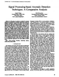
Table III summarizes the various statistics of the data sets used in our experiments. All data sets are available from our web site2 . The distribution of the symbols for normal and anomalous sequences is illustrated in Figures 1(a),1(b) (RVP), 1(c),1(d) (snd-unm), and 1(e),1(f), (bsm-week2). The distribution of symbols in snd-unm data is different for normal and anomaly data, while the difference is not significant in RVP and bsm-week2 data. We will explain how the normal and anomalous sequences were obtained for each type of data set in the next subsections. 2 http://www.cs.umn.edu/

chandola/ICDM2008

6

rvp Normal

rvp Anomaly

snd−unm Normal 0.3

0.12

0.12

0.1

0.1

0.08

0.08

0.2

0.06

0.06

0.15

0.04

0.04

0.1

0.02

0.02

0.05

0

0

5

10

15

20

25 Symbols

30

35

40

45

0

50

0.25

0

5

(a) RVP Normal

10

15

20

25 Symbols

30

35

40

45

50

0

0

10

(b) RVP Anomalous

snd−unm Anomaly

20

30 Symbols

40

50

60

(c) snd-cert Normal

bsm−week2 Normal

bsm−week2 Anomaly

0.3 0.3

0.3

0.25

0.25

0.2

0.2

0.15

0.15

0.25

0.2

0.15

0.1

0.1

0.1

0.05

0.05

0.05

0

0

10

20

30 Symbols

40

50

60

(d) snd-cert Anomalous Fig. 1.

0

0

10

20

30

40 Symbols

50

60

(e) bsm-week2 Normal

70

80

0

0

10

20

30

40 Symbols

50

60

70

80

(f) bsm-week2 Anomalous

Distribution of Symbols in Training Data Sets of Different Types.

4.1 Protein Data Sets The first set of public data sets were obtained from PFAM database (Release 17.0) [Bateman et al. 2000] containing sequences belonging to 7868 protein families. Sequences belonging to one family are structurally different from sequences belonging to another family. We choose five families, viz., HCV, NAD, TET, RVP, RUB. For each family we construct a normal data set by choosing a sample from the set of sequences belonging to that family. We then sample 50 sequences from other four families to construct an anomaly data set. Similar data was used by [Sun et al. 2006] to evaluate the PST technique. The difference was that the authors constructed a test data for each pair of protein families such that samples from one family were used as normal and samples from the other were used as test. The PST results on PFAM data sets reported in this paper appear to be worse than those reported in [Sun et al. 2006]. 4.2 Intrusion Detection Data Sets The second set of public data sets were collected from two repositories of benchmark data generated for evaluation of intrusion detection algorithms. One repository was generated at University of New Mexico3 . The normal sequences consisted of sequence of system calls generated in an operating system during the normal operation of a computer program, such as sendmail, ftp, lpr etc. The anomalous sequences consisted of sequence of system calls generated when the program is run in an abnormal mode, corresponding to the operation of a hacked computer. We report results on two data sets, viz, snd-unm and snd-cert. Other data sets were not used due to insufficient anomalous sequences to attain a 20:1 imbalance. For each of the two data sets, the number of sequences in the normal as well as anomaly data was small (less than 200), making it difficult to construct significant test and training data sets. The increase the size of the data sets, we extracted subsequences of length 100 by sliding a window of length 100 and a sliding step of 50. The subsequences extracted from the original normal sequences were treated as normal sequences and the subsequences extracted from the original anomalous sequences were treated as anomalous sequences if they did not occur in the normal sequences. The other intrusion detection data repository was the Basic Security Module (BSM) audit data, collected from a victim Solaris machine, in the DARPA Lincoln Labs 1998 network simulation data sets [Lippmann and 3 http://www.cs.unm.edu/∼immsec/systemcalls.htm

7

et al 2000]. The repository contains labeled training and testing DARPA data for multiple weeks collected on a single machine. For each week we constructed the normal data set using the sequences labeled as normal from all days of the week. The anomaly data set was constructed in a similar fashion. The data is similar to the system call data described above with similar (though larger) alphabet. The protein data sets and intrusion detection data sets are quite distinct in terms of the nature of anomalies. The anomalous sequences in a protein data set belong to a different family than the normal sequences, and hence can be thought of as being generated by a very different generative mechanism. This is also supported by the difference in the distributions of symbols for normal and anomalous sequences for RVP data as shown in Figures 1(a) and 1(b). The anomalous sequences in the intrusion detection data sets correspond to scenario when the normal operation of a system is disrupted for a short span. Thus the anomalous sequences are expected to appear like normal sequences for most of the span of the sequence, but deviate in very few locations of the sequence. Figures 1(e) and 1(f) shows how the distributions of symbols for normal and anomalous sequences in bsm-week2 data set, are almost identical. One would expect the UNM data sets (snd-unm and snd-cert) to have similar pattern as for the DARPA data. But as shown in Figures 1(c) and 1(d), the distributions are more similar to the protein data sets. 4.3 Artificial Data Sets As mentioned in the previous section, the public data sets reveal two types of anomalous sequences, one which are arguably generated from a different generative mechanism than the normal sequences, and the other which result from a normal sequence deviating for a short span from its expected normal behavior. Our hypothesis is that different techniques might be suited to detect anomalies of one type or another, or both. To confirm our hypothesis we generate artificial sequences from an HMM based data generator. This data generator allows us to generate normal and anomalous sequences with desired characteristics. We used a generic HMM, as shown in Figure 2 to model normal as well as anomalous data. The HMM

S12

S6 a6 S 5 a5

a4 S4

a1 a1

S1

a2

S2

1−λ

λ

S7 a 6

a2

S11

S 8 a5

a3

S10

a3

a4

S3

S9

Fig. 2.

HMM used to generate artificial data.

shown in Figure 2 has two sets of states, {S1 , S2 , . . . S6 } and {S7 , S8 , . . . S12 }. Within each set, the transitions corresponding to the solid arrows shown in Figure 2 were assigned a transition probability of (1−5β), while other transitions were assigned transition probability β. No transition is possible between states belonging to different sets. The only exception are S2 S8 for which the transition probability is λ, and S7 S1 for which the transition probability is 1 − λ. The transition probabilities S2 S3 and S7 S8 are adjusted accordingly so that the sum of transition probabilities for each state is 1. The observation alphabet is of size 6. Each state emits one alphabet with a high probability (1 − 5α), and all other alphabets with a low probability (α). Figure 2 depicts the most likely alphabet for each state. The initial probability vector π of the HMM is constructed such that either π1 = π2 = . . . = π6 = 1 and π7 = π8 = . . . = π12 = 0; or vice-versa. Normal sequences are generated by setting λ to a low value and π to be such that the first 6 states have initial probability set to 16 and rest 0. If λ = β = α = 0, the normal sequences will consist of the subsequence 8

a1 a2 a3 a4 a5 a6 getting repeated multiple times. By increasing λ or β or α, anomalies can be induced in the normal sequences. This generic HMM can be tuned to generate two types of anomalous sequences. For the first type of anomalous sequences, λ is set to a high value and π to be such that the last 6 states have initial probability set to 61 and rest 0. The resulting HMM is directly opposite to the HMM constructed for generating normal sequences. Hence the anomalous sequences generated by this HMM are completely different from the normal sequences. To generate second type of anomalous sequences, the HMM used to generate the normal sequence is used, with the only difference that λ is increased to a higher value than 0. Thus the anomalous sequences generated by this HMM will be similar to the normal sequences except that there will be short spans when the symbols are generated by the second set of states. By varying λ, β, and α, we generated several evaluation data sets (with two different type of anomalous sequences). We will present the results of our experiments on these artificial data sets in next section. 5. EVALUATION METHODOLOGY The techniques investigated in this paper assign an anomaly score to each test sequence Sq ∈ ST . To compare the performance of different techniques we adopt the following evaluation strategy: (1) Rank the test sequences in decreasing order based on the anomaly scores. (2) Count the number of true anomalies in the top p portion of the sorted test sequences, where p = δq, 0 ≤ δ ≤ 1, and q is the number of true anomalies in ST . Let there be t true anomalous sequences in top p ranked sequences. t (3) Accuracy of the technique = qt = δp . We experimented with different values of δ and reported consistent findings. We present results for δ = 1.0 in this paper. 6. COMPUTATIONAL COMPLEXITY Though computational complexity is an important metric when evaluating anomaly detection techniques in real application domains, we do not present a detailed comparison of computational complexity of different techniques due to space limitations. Briefly, since kernel based techniques involve computation of pairwise similarity, their computational complexity can be very high. The computation of similarity measure itself is a complex operation which can become a computational bottleneck for such techniques. Learning the model in HMM as well as RIPPER technique is expensive, though not as much as the computation of pairwise similarity for kernel based techniques. The PST technique is the most economical in terms of computational cost due to the pruning involved. t-STIDE, FSA, and FSA-z are relatively more expensive than PST though not very significantly. 7. EXPERIMENTAL RESULTS The experiments were conducted on a variety of data sets discussed in Section 4. The various parameter settings associated with each technique were explored. The results presented here are for the parameter setting which gave best results across all data sets, for each technique. The parameter settings for the reported results are : CLUSTER (c = 32), kNN (k = 4), FSA,FSA-z (n = 5, l = 1), t-STIDE (k = 6), PST (L = 6, Pmin = 0.01), RIPPER (k = 6). For public data sets, HMM was run with σ = 4, while for artificial data sets, HMM was run with σ = 12. For window based and Markovian techniques, the techniques were evaluated using different combination methods discussed in Section 3.4.The results reported here are for the average log score combination function. 7.1 Results on Public Data Sets Table IV summarizes the results on 10 public data sets.CLUSTER and kNN show good performance for PFAM and UNM data sets but perform poorly on DARPA data sets. FSA and FSA-z show consistently good performance for all public data sets. t-STIDE performs well for PFAM data sets but its performance degrades for both UNM and DARPA data sets. While PST performs average to poor for all data sets, 9

PFAM

cls knn tstd fsa fsaz pst rip hmm Avg

hcv 0.54 0.88 0.92 0.88 0.92 0.74 0.22 0.10 0.65

nad 0.46 0.64 0.74 0.66 0.72 0.10 0.02 0.06 0.42

tet 0.84 0.86 0.50 0.48 0.50 0.66 0.02 0.20 0.51

rvp 0.86 0.90 0.90 0.90 0.90 0.50 0.52 0.10 0.70

rub 0.76 0.72 0.88 0.80 0.88 0.28 0.56 0.00 0.61

Table IV.

UNM sndsndunm cert 0.76 0.94 0.84 0.94 0.58 0.30 0.82 0.88 0.80 0.88 0.28 0.10 0.76 0.74 0.00 0.00 0.60 0.60

bsmweek1 0.20 0.20 0.20 0.40 0.50 0.00 0.30 0.00 0.23

DARPA bsmbsmweek2 week3 0.36 0.52 0.52 0.48 0.36 0.54 0.52 0.64 0.56 0.66 0.10 0.34 0.34 0.58 0.02 0.20 0.35 0.50

Avg 0.62 0.70 0.59 0.70 0.73 0.31 0.41 0.07

Results for public data sets.

RIPPER performs well for UNM data sets. Overall, one can observe that the performance of techniques in general is better for PFAM data sets and on UNM data sets, while the DARPA data sets are more challenging. Though the UNM and DARPA data sets are both intrusion detection data sets, and hence are expected to be similar in nature, the results in Table IV show that the performance on UNM data sets is similar to PFAM data sets. A reason for this could be that the nature of anomalies in UNM data sets are more similar to the anomalies in PFAM data sets. 7.2 Results on Artificial Data Sets Table V summarizes the results on 6 (d1–d6) artificial data sets.The normal sequences in data set d1 were generated with λ = 0.01, β = 0.01, α = 0.01. The anomalous sequences were generated using the first setting as discussed in Section 4.3, such that the sequences were primarily generated from the second set of states. For data sets d2–d6, the HMM used to generate normal sequences was tuned with β = 0.01, α = 0.01. The value of λ was increased from 0.002 to 0.01 in increments of 0.002. The anomalous sequences for data sets d2–d6 were generated using the second setting in which λ is set to 0.1. cls knn tstd fsa fsaz pst rip hmm Avg

d1 1.00 1.00 1.00 1.00 1.00 1.00 1.00 1.00 1.00

d2 0.80 0.88 0.82 0.88 0.92 0.84 0.78 0.50 0.80

Table V.

d3 0.74 0.76 0.64 0.50 0.60 0.82 0.64 0.34 0.63

d4 0.74 0.76 0.64 0.52 0.52 0.76 0.66 0.42 0.63

d5 0.58 0.60 0.48 0.24 0.32 0.68 0.52 0.16 0.45

d6 0.64 0.68 0.50 0.28 0.38 0.68 0.44 0.66 0.53

Avg 0.75 0.78 0.68 0.57 0.62 0.80 0.67 0.51

Results for artificial data sets.

From Table V, we observe that PST is the most stable technique across the artificial data sets, while the deterioration is most pronounced for FSA and FSA-z. Both kNN and CLUSTER also get negatively impacted as the λ increases but the trend is gradual than for FSA-z. 7.3 Results on Altered RVP Data Set Third set of experiments was conducted on the RVP data set from PFAM repository. A test data set was constructed by sampling 800 most normal sequences not present in training data. Anomalies were injected in 50 of the test sequences by randomly replacing k symbols in each sequence with the least frequent symbol in the data set. The objective of this experiment was to construct a data set in which the anomalous sequences are minor deviations from normal sequences, as observed in real settings such as intrusion detection. We tested data sets with different values of k using CLUSTER, t-STIDE, FSA, FSA-z, PST, RIPPER, and HMM. Figure 3 shows the performance of the different techniques for different values of k from 1 to 10. We observe that FSA-z performs remarkably well for these values of k. CLUSTER, t-STIDE, FSA, PST, and RIPPER exhibit moderate performance, though for values of k closer to 10, RIPPER performs better than 10

the other 4 techniques. For k > 10, all techniques show better than 90% accuracy because the anomalous sequences become very distinct from the normal sequences, and hence all techniques perform comparably well. Note that the average length of sequences for RVP data set is close to 90. 100 90 80

Accuracy (%)

70 60 50 40 30 CLUSTER t-STIDE FSA FSA-z PST RIPPER HMM

20 10 0 1

2

Fig. 3.

3

4 5 6 7 Number of Anomalous Symbols Inserted (k)

8

9

10

Results for altered RVP data sets

7.4 Relative Performance of Different Techniques Kernel based techniques are found to perform well for data sets in which the anomalous sequences are relatively different from the normal sequences; but perform poorly when the different between the two is small. This is due to the nature of the normalized LCS similarity measure used in the kernel based techniques. Future work should investigate other similarity measures that are able to capture the difference between sequences that are minor deviations of each other. Our experiments show that kNN technique is somewhat better suited than CLUSTER for anomaly detection, which is expected, since kNN is optimized to detect anomalies while the clustering algorithm in CLUSTER is optimized to obtain clusters in the data. FSA-z is consistently superior among all techniques for all of the public data sets (See Table IV). The results on altered RVP data set, as shown in Figure 3 indicate that FSA-z is best suited to detect anomalous sequences that are minor deviations from the normal sequences. FSA-z is superior to FSA on all data sets. Performance of t-STIDE is comparable to FSA-z for all PFAM data sets but is relatively poor on DARPA and UNM data sets. t-STIDE performs significantly better on artificial data sets. PST performs relatively worse than other techniques on the public data sets. PST is better suited for cases where the normal sequences themselves contain many rare patterns (See Table V. RIPPER is also an average performer on most of the data sets, though it is better than t-STIDE on UNM data sets and is better than PST for most of the data sets, indicating that using a sparse history model is better than a variable history model. For the public data sets, we found the HMM technique to perform poorly. The reasons for the poor performance of HMM are twofold. The first reason is that HMM technique makes an assumption that the normal sequences can be represented with σ hidden states. Often, this assumption does not hold true, and hence the HMM model learnt from the training sequences cannot emit the normal sequences with high confidence. Thus all test sequences (normal and anomalous) are assigned a low probability score. The second reason for the poor performance is the manner in which a score is assigned to a test sequence. The test sequence is first converted to a hidden state sequence, and then a 1 + 1 FSA is applied to the transformed sequence. We have observed from our experiment using FSA that a 1 + 1 FSA does not perform well for anomaly detection. The performance of HMM on artificial data sets (Table V illustrates this argument. Since the training data was actually generated by a 12 state HMM and the HMM technique was trained with σ = 12; thus the HMM model effectively captures the normal sequences. The results of HMM for artificial data sets are therefore better than for public data sets, but still slightly worse than other techniques because of the poor performance of the 1 + 1 FSA. When the normal sequences were generated using an HMM, the 11

performance improves significantly. The hidden state sequences, obtained as a intermediate transformation of data, can actually be used as input data to any other technique discussed here. The performance of such an approach will be investigated as a future direction of research. 8. IMPACT OF NATURE OF SIMILARITY MEASURE ON PERFORMANCE OF ANOMALY DETECTION TECHNIQUES One distinction between normal and anomalous sequences is that normal test sequences are expected to be more similar (using a certain similarity measure) to training sequences, than anomalous test sequences. If the difference in similarity is not large, this characteristic will not be able to accurately distinguish between normal and anomalous sequences. This characteristic is utilized by kernel based techniques (kNN and CLUSTER) to distinguish between normal and anomalous sequences. 1000 900

400

Normal Anomalies

350

Normal Anomalies

800 300 700 600

250

500

200

400

150

300 100 200 50

100 0

0 0.43 0.48 0.52 0.57 0.61 0.66 0.70 0.75 0.79 0.84

0.76 0.77 0.78 0.79 0.80 0.81 0.82 0.83 0.84 0.85

(a) Data Set d1. Fig. 4.

(b) Data Set d6.

Histogram of Average Similarities of Normal and Anomalous Test Sequences to Training Sequences.

For example, Figure 4(a) shows the histogram of the average (nLCS) similarities of test sequences in the artificial data set d1 to the training sequences. The normal test sequences are more similar to the training sequences, than the anomalous test sequence. This indicates that techniques that use similarity between sequences to distinguish between anomalous and normal sequences will perform well for this data set. From Table V, we can observe that the performance of CLUSTER as well as kNN is 100% on d1. A similar histogram for data set d6 is shown in Figure 4(b), which shows that average similarities of normal test sequences and the average similarities of anomalous test sequences are very close to each other. This confirms the observation in Table V that CLUSTER and kNN should perform poorly for this data set. We quantify the above characteristic for kNN by computing each test sequences’ similarity to its top k th neighbor, where S is the training data set, and k is the parameter used by kNN. Let the average value of the top k similarities for normal test sequences be denoted as skn , and average value of the top k similarities for anomalous test sequences be denoted as ska . If a given data set is distinguishable in terms of sk , kNN is expected to perform well for that data set, and vice-versa. Similarly, for CLUSTER, we compute each test sequences’ average similarity with its top |S| c neighbors, where S is the training data set, and c is the parameter used by CLUSTER. Let the average value of the average similarities for normal test sequences be denoted as scn , and average value of the average similarities for anomalous test sequences be denoted as sca . If a given data set is distinguishable in terms of sc , CLUSTER is expected to perform well for that data set, and vice-versa.

sk,n sk,a sc,n sc,a

hcv 0.56 0.39 0.53 0.38

nad 0.56 0.40 0.48 0.38

Table VI.

tet 0.74 0.39 0.67 0.37

rvp 0.83 0.37 0.82 0.36

rub 0.78 0.38 0.75 0.37

sndunm 0.99 0.52 0.99 0.50

sndcert 1.00 0.39 0.99 0.38

bsmweek1 0.98 0.89 0.97 0.88

bsmweek2 0.99 0.86 0.98 0.81

Values of skn , ska , scn , sca for the public data sets.

12

bsmweek3 0.99 0.81 0.97 0.73

sk,n sk,a sc,n sc,a Table VII.

d1 0.87 0.46 0.87 0.45

d2 0.87 0.84 0.87 0.83

d3 0.87 0.83 0.86 0.83

d4 0.87 0.84 0.86 0.83

d5 0.86 0.84 0.86 0.83

d6 0.86 0.83 0.86 0.83

Values of skn , ska , scn , sca for the artificial data sets.

Tables VI and VII show the values of skn , ska , scn , sca for the real and artificial data sets, respectively. We use the observations in these tables to explain the performance of kNN and CLUSTER on different data sets. kNN. The performance of kNN on the public and artificial data sets is highly correlated with the difference sk,n − sk,a , as reported in Tables VI and VII, which confirms our hypothesis that kNN performs well for data sets which are distinguishable in terms of the characteristic sk . CLUSTER. From Table VI we observe that CLUSTER generally performs well for public data sets in which the difference sc,n − sc,a is high. For data sets such as nad, where the difference is very small, the performance of CLUSTER is poor. Similarly, from Table VII, we observe that the performance of CLUSTER is highly correlated with the difference sc,n − sc,a for the artificial data sets. 9. IMPACT OF PRESENCE OF K-WINDOWS IN SEQUENCES ON PERFORMANCE OF ANOMALY DETECTION TECHNIQUES In this section we will try to understand the behavior of the window based (t-STIDE) and Markovian techniques (FSA, FSA-z, PST, and RIPPER). These 5 techniques are related to each other since all of them analyze fixed length windows in a test sequence to determine if it is normal or anomalous. t-STIDE assigns a likelihood score to every window of size k in a given test sequence. The Markovian techniques (FSA, FSA-z, PST, and RIPPER) assign a likelihood score to each symbol in the test sequence by estimating the probability of occurrence of the symbol in the context of previous few symbols. Thus, for every symbol, both window based and Markovian techniques assign a likelihood score to a window ending with the given symbol. For t-STIDE, the window size is equal to the parameter k. For FSA and FSA-z, the window size is equal to n + l = k. For both PST and RIPPER, the window size is actually variable, but is upper bounded by a constant value (say k). To understand how each of these techniques distinguish between normal and anomalous test sequences, it is important to understand the composition of normal and anomalous test sequences in terms of the kwindows4 . The intuition behind this argument is that each of the window based and Markovian techniques assume that normal and test sequences consist of different types of k-windows in varying proportions. By assigning different scores to different k-windows, the aggregate score for a normal test sequence will be different than an anomalous test sequence, and hence the technique will be able to differentiate between the two sequences. The window based and Markovian techniques use the following two quantities to characterize a k-length window: —fk : frequency of the k-window in the training data set. —fk−1 : frequency of the k − 1 sized prefix of the k-window in the training data set. Note that, 0 ≤ fk−1 ≤ fk . From now on we will denote a k-window as w(fk , fk−1 ). Using the characteristics, fk and fk−1 , we can represent a given test sequence as a 2D histogram, where each square bin (cell) contains the number of k-windows (in the given test sequence) for which fk and fk−1 fall in the range specified by the cell. The color of each cell represents the relative proportion of k-windows falling in that cell. We refer to such a histogram for a test sequence as the frequency profile of the test sequence. The average of such histograms for all normal test sequences is the average frequency profile of normal test sequences and similarly, the average of such histograms for all anomalous test sequences is the average frequency profile of anomalous test sequences. The frequency profiles are a function of k. 4A

window of size k

13

Absolute Difference in Distribution of 5−Windows in hcv

Distribution of 5−Windows in hcv − Anomalous Sequences

488

442

442

442

393

393

393

344

344

344

0.7

295

295

295

0.6

246

246

246 fk

534

488

fk

534

488

1 0.9 0.8

0.5

0

−1

−1

−1

0.2 0.1

(b) Anomalous Test Sequences. Fig. 5.

534

488

442

393

344

295

fk−1

fk−1

(a) Normal Test Sequences.

246

197

99

148

1

50

0

0

534

0

−1

534

488

442

393

344

295

246

197

99

148

1

50

0

fk−1

−1

1

0 488

1

0

442

1

393

50

344

50

295

0.3

50

246

99

197

99

99

0.4

99

148

148

1

197

148

50

197

148

197

−1

fk

Distribution of 5−Windows in hcv − Normal Sequences 534

(c) Difference. (∆ = 1.56)

Frequency profiles for hcv data set (k = 6).

The average frequency profiles for normal and anomalous test sequences in hcv data set are shown in Figures 5(a) and 5(b), respectively5 . The absolute difference between normal and anomalous frequency profiles is shown in Figure 5(c) with marker “+” indicating that normal test sequences had higher value for that cell than the anomalous test sequences, and marker “△” indicating that normal test sequences had lower value for that cell than the anomalous test sequences. We also report the sum of the absolute values in the difference plot as ∆ (0 ≤ ∆ ≤ 2). Similar plot for snd-unm data sets is shown in Figure 6. Appendix A shows plots (differences only) for other public data sets6 . 94197

94197

Absolute Difference in Distribution of 5−Windows in snd−unm 94197

85637

85637

85637

77077

77077

77077

68513

68513

68513

59949

59949

59949

0.7

51385

51385

51385

0.6

42821

42821

42821 fk

fk

Distribution of 5−Windows in snd−unm − Anomalous Sequences

1 0.9 0.8

0.5

0

−1

−1

−1

fk−1

(a) Normal Test Sequences. Fig. 6.

0.2 0.1

(b) Anomalous Test Sequences.

94197

85637

77077

68513

59949

51385

42821

34257

25693

8565

17129

1

0

0

−1

94197

85637

77077

68513

59949

51385

42821

34257

25693

17129

8565

1

0

fk−1

94197

0 85637

1

0

77077

1

1

68513

8565

59949

8565

51385

0.3

8565

42821

17129

34257

17129

25693

0.4

17129

8565

25693

17129

25693

1

25693

0

34257

−1

34257

34257

−1

fk

Distribution of 5−Windows in snd−unm − Normal Sequences

fk−1

(c) Difference. (∆ = 1.68)

Frequency profiles for snd-unm data set (k = 6).

We observe that for the public data sets, the frequency profiles for normal and anomalous test sequences are different to varying degrees. For example, the normal and anomalous average frequency profiles are very different for the most PFAM data sets and UNM data sets, while the profiles are similar for the DARPA data sets. Another general observation is that the data sets for which the normal and anomalous test sequences are significantly different (such as hcv, rvp, snd-cert, snd-unm), the performance of t-STIDE and Markovian techniques is better, while the data sets for which the normal and anomalous test sequences are not significantly different (such as tet, bsm-week1, bsm-week2, bsm-week3), the performance of these techniques is poor. The correlation between the performance of the window based and Markovian techniques and the difference between normal and anomalous frequency profiles, motivates our next question, i.e., why some window based/Markovian techniques perform better on a given data set while others perform poorly? A simple answer is that different techniques assign a different likelihood score to every cell (and hence to the kwindows belonging to the cell) in the frequency profile of a test sequence. A technique which assigns higher 5 All

plots are best viewed in color. resolution plots are available at www.cs.umn.edu/∼chandola/SEQ/

6 Higher

14

Technique t-STIDE FSA

Table VIII.

L(w(fk , fk−1 )) ∝ fk f = f k

FSA-z

=

PST

≥

RIPPER

≥

No score is assigned if fk = fk−1 = 0

k−1 fk fk−1 fk fk−1 fk fk−1

If fk = fk−1 = 0, L(fk , fk−1 ) = 0

Likelihood scores assigned by different techniques to a given k-window, w(fk , fk−1 ).

likelihood scores to the cells which contain a high proportion of k-windows belonging to normal sequences, and lower likelihood scores to the cells which contain a high proportion of k-windows belonging to anomalous sequences, will be able to better distinguish between normal and anomalous test sequences. To explain the above answer in a more systematic manner let us consider a data set and a particular technique. Let the frequency profile of a normal test sequence be denoted as Fn and the frequency profile of an anomalous test sequence be denoted as Fa . Let L denote the matrix of likelihood scores assigned by the given technique to different cells in the frequency profile. Then the likelihood score assigned by the technique to a normal test sequence L(Sn ) is approximately equal to: XX L(Sn ) = Fn [ij]L[ij] (3) i

j

Similarly, the likelihood score assigned by the technique to anomalous test sequence L(Sa ) is approximately equal to: XX L(Sa ) = Fa [ij]L[ij] (4) i

j

The objective of any technique is to assign a higher likelihood score to a normal test sequence and a lower likelihood score to an anomalous test sequence, in order to distinguish between the two. In order to achieve this, the technique should assign a higher score to L[ij] if Fn [ij] >> Fa [ij] and should assign a lower score to L[ij] if Fn [ij]