Understanding Network Behavior by Structured Representations of Transition Invariants A Petri Net Perspective on Systems and Synthetic Biology Monika Heiner
Abstract Petri nets offer a bipartite and concurrent paradigm, and consequently represent a natural choice for modeling and analyzing biochemical networks. We introduce a Petri net structuring technique contributing to a better understanding of the network behavior and requiring static analysis only. We determine a classification of the transitions into abstract dependent transition sets, which induce connected subnets overlapping in interface places only. This classification allows a structured representation of the transition invariants by network coarsening. The whole approach is algorithmically defined, and thus does not involve human interaction. This structuring technique is especially helpful for analyzing biochemically interpreted Petri nets, where it supports model validation of biochemical reaction systems reflecting current comprehension and assumptions of what has been designed by natural evolution.
1 Motivation Systems and synthetic biology are concerned with understanding biochemical processes (pathways) in biological systems ranging in size from a single pathway to a whole organism, and varying in the chosen abstraction level from gene regulatory networks via signal transduction networks to metabolic networks. Independently of size and abstraction level, all pathways and, therefore, their models, too, exhibit inherently rather complex network structures. These structures reflect the causal interplay of the basic actions and employ all the patterns well known in computer engineering, such as sequence, branching, repetition, and concurrency. However, opposite to technical networks, biochemical networks tend to be very dense and apparently unstructured making the understandability of the full network of interactions difficult and, therefore, error-prone. M. Heiner (!) Department of Computer Science, Brandenburg University of Technology, Postbox 101344, 03013 Cottbus, Germany e-mail:
[email protected] Fax: +49-355-693587 A. Condon et al. (eds.), Algorithmic Bioprocesses, Natural Computing Series, DOI 10.1007/978-3-540-88869-7_19, © Springer-Verlag Berlin Heidelberg 2009
367
368
M. Heiner
Getting a survey on the current state of knowledge about a particular pathway requires a lot of reading and search through several data bases, including the creative interpretation of various graphical representations. These pieces of separate understanding have to be assembled to get a comprehensive as well as consistent knowledge representation. For this purpose, a readable and executable language with a formal, and hence unambiguous semantics would obviously be of great help as a common intermediate representation language. Formal models open the door to mathematically founded analyses. The transformation from an informal to a formal model involves the resolution of any ambiguities, which must not necessarily happen in the right way. Therefore, the next step in a sound model-based technology should be devoted to model validation. Model validation aims basically at increasing our confidence in the constructed model. There is no doubt that this should be a prerequisite before raising more sophisticated questions, where the answers are supposed to be found by help of the model and where we are usually ready to trust the answers we get. So, before thinking about model-based behavior prediction, we are concerned with model validation. For model validation, we introduce a qualitative model as a supplementary intermediate step, at least from the viewpoint of the biochemist accustomed to continuous modeling only. One of the benefits of using the qualitative approach is that systems can be modeled and analyzed without any quantitative parameters. This model-driven perspective is equally helpful in the setting of systems biology as well as synthetic biology. In systems biology, models help us in formalizing our understanding of what has been created by natural evolution. So first of all, models serve as an unambiguous representation of the acquired knowledge and help to design new wetlab experiments to sharpen our comprehension. In synthetic biology, models help us to make the engineering of biology easier and more reliable. Models serve as blueprint for novel synthetic biological systems. Their employment is highly recommended to guide the design and construction in order to ensure that the behavior of the synthetic biological systems is reliable and robust under a variety of conditions. Computer science has generated quite a number of modeling formalisms, which are used in the scenario sketched so far. In this paper, we apply the Petri net formalism. Biochemical reaction systems and Petri nets share two distinctive characteristics. Both are inherently bipartite, and both are inherently concurrent. Thus, Petri nets seem to be a natural choice for modeling biochemical networks. Petri nets are known to combine an intuitive and executable modeling style with mathematically founded analysis techniques, comprising qualitative as well as quantitative ones, complemented by reliable tool support. This paper is based on a typical static analysis technique, the invariants. Place and transition invariants are a popular validation technique for technical as well as biochemical networks. One approach of acquiring a deeper understanding of the network behavior consists in understanding all its basic executions, which correspond to the minimal transition invariants. We go one step further by guiding the hierarchical structuring (coarsening) of a given network to support its comprehension. We
Understanding Network Behavior by Structured Representations of Transition Invariants
369
determine a classification of the transitions into abstract dependent transition sets, which induce connected subnets overlapping in interface places only. This classification allows a structured representation of the transition invariants by network coarsening. The whole approach is algorithmically defined, and thus does not involve human interaction. This structuring technique is especially helpful for analyzing biochemically interpreted Petri nets, where it supports model validation of biochemical reaction systems reflecting current comprehension and assumptions. This paper is organized as follows. In the next section, we recapitulate the relevant Petri net notions, before we motivate a biochemical interpretation of Petri nets. Thereafter, we introduce a new structuring method, sketch the computation of its two main features, and demonstrate the gained structuring effect by three smaller cases studies, which are also provided on our web pages. Finally, we refer to related work, before concluding with a short summary of the essential aspects.
2 Preliminaries To be self-contained, we give the formal definitions of the Petri net notions relevant for this paper. As usual, we denote the set of non-negative integers including zero by N0 , and the set of integers by Z. |S| denotes the number of elements in a set S. To allow formal reasoning, we are going to represent biochemical networks by Petri nets, which enjoy formal semantics amenable to mathematically sound analysis techniques. The first two definitions introduce the standard notion of place/transition Petri nets, which is the basic class in the ample family of Petri net models. Definition 1 (Petri Net, Syntax) A Petri net is a quadruple N = (P , T , f, m0 ), where – P and T are finite sets with P ∪ T "= ∅, P ∩ T = ∅, – f : ((P × T ) ∪ (T × P )) → N0 , – m0 : P → N0 . Thus, Petri nets (or nets for short) are weighted, directed, bipartite graphs. The elements of the set P are called places, graphically represented by circles, while the elements of the set T are called transitions, represented by rectangles. The function f defines the set of directed arcs, weighted by non-negative integers. The (pseudo) arc weight 0 stands for the absence of an arc. The arc weight 1 is the default value and is usually not given explicitly. A place carries an arbitrary number of tokens, represented as black dots or a natural number. The number zero is the default value and usually not given explicitly. m(p) yields the number of tokens on place p in the marking m, and m0 specifies the initial marking. We introduce the following notions and notations for a node x ∈ P ∪ T . – • x := {y ∈ P ∪ T | f (y, x) "= 0} is the preset of x.
370
– – – –
M. Heiner
x • := {y ∈ P ∪ T | f (x, y) "= 0} is the postset of x. x is called input node of the net if • x = ∅. x is called output node of the net if x • = ∅. x is called boundary node of the net if it is either input or output node.
Additionally, we extend the first two to a set of nodes X ⊆ P ∪ T and ! notions • X := • x, and the set of all post-nodes X • := define the set of all pre-nodes x∈X ! • x∈X x . Up to now, we have introduced the static aspects of a Petri net only. The behavior of a net is defined by the firing rule, which basically consists of two parts: the precondition and the firing itself. Definition 2 (Firing Rule) Let N = (P , T , f, m0 ) be a Petri net.
– A transition t is enabled in a marking m, written as m[t), if ∀p ∈• t : m(p) ≥ f (p, t), else disabled. – A transition t, which is enabled in m, may fire. – When t in m fires, a new marking m, is reached, written as m[t)m, , with ∀p ∈ P : m, (p) = m(p) − f (p, t) + f (t, p). – The firing happens atomically and does not consume any time.
According to this may firing rule, a transition is never forced to fire. Figuratively, the firing of a transition moves tokens from its pre-places to its post-places, while possibly changing the number of tokens; compare Fig. 1. Generally, the firing of a transition changes the formerly current marking to a new reachable one, where some transitions are not enabled anymore while others get enabled. The repeated firing of transitions establishes the behavior of the net. The whole net behavior consists of all possible partially ordered firing sequences (partial order semantics) or all possible totally ordered firing sequences (interleaving semantics), respectively. Every marking m is defined by the given token situation in all places, i.e. m ∈ |P | N0 . All markings, which can be reached from a given marking m by any firing sequence of arbitrary length, constitute the set of reachable markings [m). The set of markings [m0 ) reachable from the initial marking is said to be the state space of a given system. However, in this paper, we confine ourselves deliberately to analysis techniques, which do not require the generation of the state space. So, the presented approach works also for nets with infinite state spaces, i.e. for unbounded Petri nets. To open the door to analysis techniques based on linear algebra (or better: discrete computational geometry), we represent the net structure by a matrix, called incidence matrix in the Petri net community and stoichiometric matrix in systems biology. We briefly recall the essential technical terms. Definition 3 (P-Invariants, T-Invariants) Let N = (P , T , f, m0 ) be a Petri net.
– The incidence matrix of N is a matrix C : P × T → Z, indexed by P and T , such that C(p, t) = f (t, p) − f (p, t). – A place vector (transition vector) is a vector x : P → Z, indexed by P (y : T → Z, indexed by T ).
Understanding Network Behavior by Structured Representations of Transition Invariants
371
– A place vector (transition vector) is called a P-invariant (T-invariant) if it is a nontrivial non-negative integer solution of the homogeneous linear equation system x · C = 0 (C · y = 0). – The set of nodes corresponding to an invariant’s non-zero entries are called the support of this invariant x, written as supp(x). – An invariant x is called minimal if " ∃ invariant z : supp(z) ⊂ supp(x), i.e. its support does not contain the support of any other invariant z, and the greatest common divisor of all non-zero entries of x is 1. – A net is covered by P-invariants, shortly CPI (covered by T-invariants, shortly CTI) if every place (transition) belongs to a P-invariant (T-invariant). Invariants are vectors over natural numbers, which can be read as specifications of multisets. Contrary, supports are sets, which can technically be specified as vectors over Booleans, which allows the access to the ith entry by indexing. The set X of all minimal P-invariants (T-invariants) xi of a given net is unique and represents a generating system for all P-invariants (T-invariants). " All invariants x can be computed as non-negative linear combinations: n · x = (ai · xi ), with n, ai ∈ N0 , i.e. the allowed operations are addition, multiplication by a natural number, and division by a common divisor.
3 Biochemically Interpreted Petri Nets The idea to use Petri nets for the representation of biochemical networks is rather intuitive and has been mentioned by Carl Adam Petri himself in one of his internal research reports on interpretation of net theory in the seventies. It has also been used as the very first introductory example in one of the early survey papers [28]. We follow this approach; see Fig. 1. Places usually model passive system components like conditions, species, or any kind of chemical compounds, e.g. proteins or proteins complexes, playing the role of precursors, products, or enzymes of chemical reactions. Occasionally, we want to differentiate between primary and secondary compounds. The latter ones are often assumed to be ubiquitous and available in sufficient amount. Complementary, transitions stand usually for active system components like atomic actions or any kind of chemical reactions, e.g. association, dissociation, phosphorylation, or dephosphorylation, transforming precursors into products, possibly controlled by enzymes. A reversible chemical reaction is modeled by two opposite transitions; compare Fig. 2.
Fig. 1 The Petri net for the well-known chemical reaction r: 2H2 + O2 → 2H2 O and three of its markings (states), connected each by a firing of the transition r. The transition is not enabled anymore in the marking reached after these two single-firing steps
372
M. Heiner
Fig. 2 Hierarchical structuring by use of macro transitions, which are drawn as two centric squares. The flat net (left) and the hierarchical net (right) are identical—from an analysis point of view. Both nets model a reversible reaction a ! b with its producing and consuming environment. The nodes colored in gray may be considered as logical nodes, automatically generated by the drawing tool. They connect the transition-bordered subnet on the lower hierarchy level with its environment on the next higher hierarchy level
The arcs go from precursors to reactions (ingoing arcs), and from reactions to products (outgoing arcs). In other words, the pre-places of a transition correspond to the reaction’s precursors, and its post-places to the reaction’s products. Enzymes establish side conditions and are connected in both directions with the reaction they catalyze – we get read arcs; compare place O2 in Fig. 6. Arc weights may be read as the multiplicity of the arc, reflecting known stoichiometries. Tokens can be interpreted as the available amount of a given species in number of molecules or moles, or any abstract, i.e. discrete concentration level. We adopt the following drawing conventions; compare Fig. 2. – Input/output transitions are generally drawn as flat rectangles to highlight their special meaning for the net behavior. – Logical nodes (fusion nodes) are colored in gray. All logical nodes with the same name are identical, at least from an analysis point of view. They are commonly used for compounds involved in many reactions, e.g. secondary compounds. – Transition-bordered subnets can be hidden in macro transitions, drawn as two centric squares. This allows an hierarchical structuring of larger nets. We are going to apply this technique to coarsen a given net according to its minimal T-invariants’ inherent structure; see Sect. 4. Invariants are a beneficial technique in model validation, and the challenge is to check all invariants for their biological plausibility. A P-invariant x is a non-zero and non-negative integer place vector such that x · C = 0; in words, for each transition it holds that: multiplying the P-invariant with the transition’s column vector yields zero. Thus, the total effect of each transition on the P-invariant is zero, which explains its interpretation as a token conservation component. A P-invariant stands for a set of places over which the weighted sum of tokens is constant and independent of any firing, i.e. for any markings m1 , m2 , which are reachable by the firing of transitions, it holds that x · m1 = x · m2 . In the context of metabolic networks, P-invariants reflect substrate conservations, while in signal transduction or gene regulatory networks P-invariants often correspond to
Understanding Network Behavior by Structured Representations of Transition Invariants
373
the several states of a given species (protein or protein complex) or gene. A place belonging to a P-invariant is obviously bounded, and CPI causes structural boundedness, i.e. boundedness for any initial marking. Analogously, a T-invariant y is a non-zero and non-negative integer transition vector such that C · y = 0; in words, for each place it holds that: multiplying the place’s row with the T-invariant yields zero. Thus, the total effect of the T-invariant on a marking is zero. A T-invariant has two interpretations in the given biochemical context. – The entries of a T-invariant specify a multi-set of transitions, which by their partially ordered firing reproduce a given marking, i.e. basically occurring one after the other. This partial order sequence of the T-invariant’s transitions may contribute to a deeper understanding of the net behavior. A T-invariant is called feasible if such a behavior is actually possible in the given marking situation. – The entries of a T-invariant may also be read as the relative firing rates of the transitions involved, all of them occurring permanently and concurrently. This activity level corresponds to the steady state behavior. The two opposite transitions modeling the two directions of a reversible reaction always make a minimal T-invariant; thus, they are called trivial T-invariants. A net which is covered by non-trivial T-invariants is said to be strongly covered by T-invariants (SCTI). Transitions not covered by non-trivial T-invariants are candidates for model reduction, e.g. if the model analysis is concerned with steady state analysis only. The automatic identification of non-trivial minimal T-invariants is in general useful as a method to highlight important parts of a network, and hence aid its comprehension by biochemists, especially when the entire network is too complex to easily comprehend. We are especially interested in a network’s input/output behavior, which we are going to characterize by input/output T-invariants (I/O T-invariants), i.e. such T-
Fig. 3 The four nets on the left are each covered by one minimal T-invariant. Invariants can contain any structures (from left to right): cycles, forward/backward branching transitions, forward branching places, backward branching places. Generally, invariants overlap, and in the worst-case there are exponentially many of them; the net on the far-right has 24 T-invariants
374
M. Heiner
invariants, involving input and output transitions. These special T-invariants can often be read as alternative, self-contained pathways within a given network under consideration. A minimal P-invariant (T-invariant) defines a connected subnet, consisting of its support, its pre- and post-transitions (pre- and post-places), and all arcs in between. There are no structural limitations for such subnets induced by minimal invariants, compare Fig. 3, but they are always connected, however, not necessarily strongly connected. These minimal self-contained subnets may be read as a decomposition into token preserving or state repeating modules, which should have an enclosed biological meaning. Minimal invariants generally overlap; the combinatorial effect causes an explosion of the number of minimal invariants. There are exponentially many of them in the worst-case; compare Fig. 3, far-right. Therefore, we are going to apply a structured representation of a given set of invariants.
4 Structuring Method The following discussion concentrates on T-invariants. Likewise, the presented technique can be applied to P-invariants due to the given symmetry of the two notions. We define a dependency relation based on a set of minimal T-invariants. It can be equally applied to the full set of all minimal T-invariants as well as to a subset, e.g. the set of non-trivial T-invariants. Definition 4 (Dependency Relation) Let N = (P , T , f, m0 ) be a Petri net, and let Y denote a set of minimal T-invariants y of N . Two transitions i, j ∈ T depend on each other, i 01 j for short, if ∀y ∈ Y : i ∈ supp(y) ⇔ j ∈ supp(y). This is an abstract dependency, defined on the T-invariants’ support only. Dependent transitions appear always together in the given set of minimal T-invariants. The drop out of one transition prevents the whole set of transitions depending on each other to accomplish their common function. The dependency relation fulfills the following properties: – reflexivity: i 01 i; – a transition depends on its own. – symmetry: i 01 j ⇔ j 01 i; the dependency of i on j implies the dependency of j on i, and vice versa. – transitivity: i 01 j ∧ j 01 k ⇒ i 01 k; if i depends on j , and j depends on k, then i depends also on k. Thus, it is an equivalence relation in the transition set T , leading to a partition of T . We call the equivalence classes Ai with Ai ⊆ T ∧ ∪Ai = T ∧ ∀i, j : i "= j ⇒ Ai ∩ Aj = ∅
Understanding Network Behavior by Structured Representations of Transition Invariants
375
maximal abstract dependent transition sets (ADT sets), and it holds ∀Ai , ∀y ∈ Y : Ai ⊆ supp(y) ∨ Ai ∩ supp(y) = ∅. ADT sets can be read as the smallest biologically meaningful functional units (building blocks). Contrary to T-invariants, which generally overlap, ADT sets induce by definition subnets overlapping in interface places pif ∈ PIF only, with PIF =
#
∀i,j,i"=j
(• Ai ∪ Ai • ) ∩ (• Aj ∪ Aj • ).
These subnets represent a possible structural decomposition of biochemical networks into smaller subnets. Notably, the decomposition is based on statically decidable properties only. Following the idea of hierarchical structuring of larger networks, we are going to hide building blocks within macro transitions. However, ADT sets are not necessarily connected, as we will see in Sect. 6. Hence, a further decomposition into connected ADT sets is generally needed, possibly according to primary compound flow only, i.e. neglecting connections by secondary compounds, and we get nonmaximal ADT sets. Having a decomposition of the transition set T into ADT sets inducing connected subnets, we are able to determine the interface places, and to coarsen automatically a given net according to the minimal T-invariants’ inherent structure: – macro transitions abstract from connected ADT sets, and – places on the hierarchy’s top level correspond to the interface between the ADT sets. Then the coarse net structure gives a structured representation of all T-invariants, which may contribute to a better understanding of the net behavior. Moreover, the coarse net structure allows to identify sensitive net parts, i.e. interface places; the knock-out of which would switch off a significant part of the whole network or even prevent any output. Maximal ADT sets support also the efficient design of wetlab experiments by identifying minimal sets of observation points providing coverage of the whole network: each maximal ADT set needs obviously one observation point only. Finally, ADT sets are likely to be useful for automatic layout algorithms, whereby the differentiation between primary and secondary compounds might be supportive.
5 Computation For the algorithmic-oriented minds, we sketch the computation of the two main features of which our structuring approach is made.
376
M. Heiner
5.1 Computation of Invariants Technically, we need to solve a homogeneous linear equation system over nonnegative integers. This restriction of the data space establishes—from a strong mathematical point of view—a challenge. There is no closed formula to compute the solutions. However, there are algorithms—actually, a class of algorithms— constructing the solution (to be precise: the generating system for the solution space) by systematically considering all possible candidates. This algorithm class has been repetitively re-invented over the years. Thus, these algorithms come along with different names. But a closer look always reveals the same underlying principle. All these versions may be classified as “positive Gauss elimination”; the incidence matrix of the Petri net is systematically transformed to a zero matrix by suitable matrix operations. Before we start, an auxiliary matrix is added to the incidence matrix to log, which matrix operations have been done. The auxiliary matrix is always a quadratic matrix. It is initialized by the identity matrix (diagonal is set to 1, else 0), and it is added to the right for the computation of the P-invariants (then it is a quadratic matrix over the places), or it is added below the incidence matrix for the computation of the Tinvariants (then it is a quadratic matrix over the transitions). The matrix operations, compare Algorithm 1, are always applied to the composed matrix, consisting of the incidence matrix and the auxiliary matrix. The algorithm terminates, when all columns in the incidence matrix are zero. It needs at most as many iterations of the outer loop as we have transitions, because each iteration makes one column to zero. Algorithm 1 Computation of P-invariants input incidence matrix C, extended by auxiliary matrix; while there are non-zero columns in C do pick one non-zero column i in C; for all pairs of rows with unequally signed entries in this column i do add a new row, which is the smallest possible linear combination of this pair, making the matrix entry in this column i to zero; end for; delete all old rows, i.e. those which have been used in creating these linear combinations; assert i is now a zero column; assert if we had n negative entries and p positive entries in column i, then the number of rows changes by n · p − (n + p) end while; assert if there is a solution, the incidence matrix is now zero; assert all rows in the auxiliary matrix are P-invariants, among them are all minimal P-invariants;
Understanding Network Behavior by Structured Representations of Transition Invariants
377
The challenge in implementing this basic algorithm is twofold. First, we need to eliminate efficiently all non-minimal P-invariants. Second, because the algorithm has to consider all possible candidates, all possible linear combinations are constructed, blowing up the number of rows in the intermediate data structure. There are heuristics trying to minimize this effect, e.g. to pick a column, for which we get less new rows. However, as we know, heuristics never work fine for all possible cases. To give some figures: It might be that there are several millions of rows at an intermediate state of the algorithm, and at the end there are just around 100 left. It is straightforward to adjust this algorithm to compute T-invariants; or the incidence matrix is transposed—P-invariants of the transposed net are the T-invariants of the original net.
5.2 Computation of Dependent Sets The algorithm is rather straightforward and easily explained. Let us recall, Tinvariants are technically transition vectors over natural numbers, i.e. they have as many components as there are transitions in the net, usually given as column vectors. Likewise, their supports can be given as transition vectors over Booleans with true if the transition belongs to the set, and false else; again written as column vectors. Let us arrange these column vectors of all T-invariants or of their supports side by side. We get a matrix Tinv with as many rows as we have transitions and as many columns as we have T-invariants. The dependency relation can now be rephrased in terms of this matrix Tinv : two transitions dependent on each other, i.e. they always occur together, if their rows are identical. Maximal dependent transition sets are now defined by maximal sets of identical rows. To compute them, we execute Algorithm 2. The algorithm terminates when all rows have been assigned. Because we have a finite set of transition, the number of rows is finite, too. In the worst case, the outer Algorithm 2 Computation of maximal dependent transition sets input matrix Tinv ; while there are non-assigned rows do create a new set s; let i be the first index of a row, which has not been assigned to a set; mark row i as assigned, and put i into s; for all non-assigned rows j do if rows i, j are identical, i.e. Tinv (i, ∗) = Tinv (j, ∗) then j belongs to the same set as i: mark j as assigned, and put j into s end if end for; assert s specifies a maximal ADT set; end while
378
M. Heiner
loop is entered as often as there are transitions. Then each transition builds its own set.
6 Case Studies We present deliberately three smaller case studies, allowing to be easily understood.
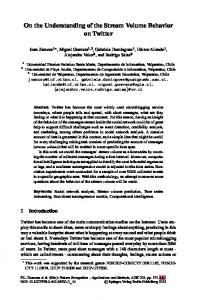
6.1 Glycolysis We start with one of the standard examples of metabolic networks, the combined glycolysis and pentose phosphate pathway in erythrocytes (red blood cell). We use a version based on [38], which is also elaborated in [19]. The network defines the various reactions occurring in the cell under heavy energy load, such as in brisk muscle activity. Glucose serves as precursor, and Lactate as product, involving several secondary compounds (ATP, ADP, NADH+, NADH, Pi) in the stepwise conversion process; compare Fig. 4. There are three minimal T-invariants, which we give in a short-hand notation, enumerating the non-zero entries only: y1 = (p_Gluc, 2 · p_ADP, 2 · p_Pi,
r9, r10, r11, r12, r13, 2 · r15, 2 · r16, 2 · r17, 2 · r18, 2 · r19, 2 · r20, 2 · c_Lac, 2 · c_ATP),
y2 = (3 · p_Gluc, 5 · p_ADP, 5 · p_Pi,
3 · r9, 6 · r1, 6 · r2, 3 · r3, 2 · r4, r5, r6, r7, r8,
2 · r11, 2 · r12, 2 · r13, 5 · r15, 5 · r16, 5 · r17, 5 · r18, 5 · r19, 5 · r20, 5 · c_Lac, 5 · c_ATP),
y3 = (r13, r14).
The net is CTI, however, not SCTI, because r14 is involved in a trivial T-invariant only. Considering the two non-trivial minimal T-invariants, y1 and y2 , we find four maximal ADT sets. The first set contains the intersection of both T-invariants, comprising almost the whole glycolysis A = supp(y1 ) ∩ supp(y2 )
= {p_Gluc, p_ADP, p_Pi,
r9, r11, r12, r13, r15, r16, r17, r18, r19, r20, c_Lac, c_ATP}.
The knock-out of one of the transitions in A switches off both non-trivial Tinvariants. The next two sets contain those transitions, which are specific to one
Understanding Network Behavior by Structured Representations of Transition Invariants
379
Fig. 4 The Petri net and its coarse structure for the combined glycolysis and pentose phosphate pathway in erythrocytes. The layout of the flat net mimics the hypergraph given in [38]. Nodes colored in gray in the flat net are logical (fusion) nodes. Input and output transitions are drawn as flat rectangles. The two pathways highlighted in the coarse net are: (a) glycolysis, and (b) pentose phosphate pathway
of the two T-invariants. The specific transition of the T-invariant y1 belongs to the glycolysis B = supp(y1 ) − supp(y2 ) = {r10},
and the specific transitions of the T-invariant y2 cover the pentose phosphate pathway C = supp(y2 ) − supp(y1 )
= {r1, r2, r3, r4, r5, r6, r7, r8}.
380
M. Heiner
The remaining transition belongs to a trivial T-invariant only; it builds an (pseudo) ADT set on its own. This transition does not contribute to the steady state behavior of the two non-trivial T-invariants. D = T − supp(y1 ) − supp(y2 ) = {r14}
Thus, the main building blocks of the Petri net, and by this way of the underlying biochemical network, are represented by the first three ADT sets, each defining a connected subnet. The two subnets, describing the two pathways, are defined by the union of the first ADT set with the second or third one, respectively. However, if we neglect the connectivity established by secondary compounds, the ADT set A breaks down into two subsets: A1 = {p_Gluc, r9},
A2 = A − A1,
which are connected according to the primary compound flow, however, not maximal anymore. We obtain the coarse network structure as given in Fig. 4, lower part, highlighting the structuring principle inherent in the non-trivial minimal T-invariants. Each macro transition stands for a connected subnet defined by a set of transitions, occurring together in all non-trivial minimal T-invariants. In this example, each elementary (loop-free) macro transition sequence in the coarse net structure corresponds to a non-trivial minimal T-invariant of the whole network. There are two such sequences: y1 = (A1; B; A2),
y2 = (A1; C; A2), sharing the beginning and the end. Thus, the two I/O T-invariants y1 , y2 are now represented by I/O macro transition sequences. The places shown in the coarse net structure are the boundary places of the subnets, building the interface between the subnets. Please note, only the primary compound flow is represented here.
6.2 Apoptosis The term apoptosis refers to the genetically programmed cell death, which is an essential part of normal physiology for most metazoan species. Disturbances in the apoptotic process may lead to various diseases. The signal transduction network of apoptosis governs complex mechanisms to control and execute programmed cell death, which are—by the time being—not really well understood. A variety of different cellular signals initiate activation of apoptosis in distinctive ways, depending on the various cell types and their biological states. We consider here a core model
Understanding Network Behavior by Structured Representations of Transition Invariants
381
Fig. 5 The Petri net and its coarse structure for a core model of the apoptosis. The layout of the flat net is inspired by the graphical scheme given in [27]. The three pathways highlighted in the coarse net are: (a) the Fas receptor pathway, (b) the pathway induced by intrinsic apoptotic stimuli, and (c) the cross-talk pathway. The ADT sets C1 and C2 are involved in all three pathways
of [16], which is based on [27], comprising the pathways induced by the Fas receptor and the intrinsic apoptotic stimuli, as well as the cross-talk in between; compare Fig. 5.
382
M. Heiner
There are three minimal T-invariants, covering the net: y1 = (p1, p2, p3, p8, p9, p10, r1, r2, r3, r4,
c1, c2, c3, c4), y2 = (p4, p5, p6, p7, p8, p9, p10,
r3, r4, r7, r8, r9, r10, r11, r12, r13, c1, c2, c3, c4),
y2 = (p1, p2, p3, p5, p6, p7, p8, p9, p10, p11, r1, r3, r4, r5, r6, r9, r10, r11, r12, r13, c1, c2, c3, c4). There are no trivial T-invariants; so, CTI implies SCTI. We consider all minimal T-invariants, and we get six maximal ADT sets: A = {p1, p2, p3, r1}, B = {r2},
C = {p8, p9, p10, r3, r4, c1, c2, c3, c4},
D = {p4, r7, r8},
E = {p5, p6, p7, r9, r10, r11, r12, r13}, F = {p11, r5, r6}.
Notably, the ADT set C is involved in all minimal T-invariants; so, it is vital for the whole network. This set does not induce a connected subnet; therefore, we decompose it into two connected subsets: C1 = {p9, p10, r3, r4, c1, c2, c3, c4}, C2 = {p8}.
Consequently, C1 and C2 are not maximal ADT sets anymore. Using these seven ADT sets, we get the coarse net structure as given in Fig. 5, lower part. The three pathways are clearly distinguishable, and—we claim—much better readable than in the flat net. In this example, each minimal I/O T-invariant is represented by a partially ordered I/O macro transition sequence in the coarse net structure (the sign + stands for ‘unordered’, i.e. concurrent macro transitions): y1 = (A + C2; B; C1),
y2 = (C2 + D; E; C1),
y3 = ((A; F) + C2; E; C1).
Understanding Network Behavior by Structured Representations of Transition Invariants
383
6.3 Hypoxia Oxygen is an essential and vital element for the survival of organisms. Lower oxygen content, termed hypoxia, arises under pathophysiological conditions. When there is an imbalance of oxygen content, the organism adapts by restoring normal oxygen content through activation of various genetic and metabolic pathways to compensate for the imbalance. One of the well-studied molecular pathways activated under hypoxia condition is the Hypoxia Induced Factor (HIF) pathway responsible for regulating oxygen-sensitive gene expression. Continuous models in the style of ordinary differential equations (ODEs) have been proposed in [21] and [51]. The Petri net given in Fig. 6 has been derived from these ODEs in order to highlight the ODEs’ inherent structure. Reading the given qualitative Petri net as a continuous Petri net, whereby all transitions firing rates follow the mass action kinetics, generates exactly the original ODEs. Here, we confine ourselves to the very first step—understanding the essential network behavior. We start with the computation of the minimal T-invariants. Besides the expected seven trivial T-invariants for the seven reversible reactions, y1 = (r3, r4),
y4 = (r15, r16), y7 = (r29, r30),
y2 = (r5, r6),
y5 = (r18, r19),
y3 = (r12, r13), y6 = (r21, r22),
there are three non-trivial ones: y8 = (r1, r2),
y9 = (r1, r12, r14, r18, r20),
y10 = (r1, r3, r15, r17, r18, r20, r22). Please note, (r1, r2) is not considered to be a trivial T-invariant due to its relevance for the input/output behavior. Determining the maximal ADT sets over all T-invariants yields 17 sets, 15 of them contain just one transition, and the remaining two are {r5, r6} and {r29, r30}, i.e. they correspond to those two trivial T-invariants, the transitions of which are not involved in any of the non-trivial T-invariants. Neglecting the trivial T-invariants in the computation of the maximal ADT sets yields the much more interesting result: A = {r1},
B = {r2},
E = {r3, r15, r17, r22},
C = {r12, r14},
D = {r18, r20},
and the pseudo ADT set, containing all remaining transitions of the net, not contributing to the non-trivial T-invariants. The maximal ADT sets A–E induce connected subnets, and we get the coarse net structure as given in Fig. 6, lower part.
384
M. Heiner
Fig. 6 The Petri net and its coarse structure (when neglecting the trivial T-invariants) for the hypoxia response network based on the ODEs given in [21] and [51]. The three pathways to degrade HIF (S3) highlighted in the coarse net are: (a) direct degradation by r2, (b) degradation not requiring S4, and (c) degradation requiring S4. The knock-out of S12 interrupts both (b) and (c)
The three non-trivial T-invariants are represented by the three macro transition sequences: y8 = (A; B),
y9 = (A; C; D),
y10 = (A; E; D).
7 Tools The case studies have been done using Snoopy [18, 45]—a tool to design and animate or simulate hierarchical graphs, among them the qualitative Petri nets as used
Understanding Network Behavior by Structured Representations of Transition Invariants
385
in this paper. Snoopy provides export to various analysis tools as well as import and export of the Systems Biology Markup Language (SBML) [13]. The T-invariants, ADT sets and their decomposition into connected subnets have been computed with the Petri net analysis tool Charlie [3]. To support result evaluation, node sets, as specified by T-invariants or ADT sets, can be visualized (colored) in Snoopy. The automatic derivation of the hierarchical Petri net showing the coarse net structure is subject of a running student’s project. The data files of the case studies and the analysis results are available at www-dssz.informatik.tu-cottbus.de/examples/coarsening.
8 Related Work Please note, the following remarks are not meant to be exhaustive, but to give the interested reader some suggestions where to continue reading. Petri nets, as we understand them today, have been initiated by concepts proposed by Carl Adam Petri in his Ph.D. thesis in 1962 [33]. The first substantial results making up the still growing body of Petri net theory appeared around 1970. Initial textbooks devoted to Petri nets were issued in the beginning of the 80s [34, 39, 47]. General introductions into Petri net theory can be found, for example, in [1, 6, 28, 48]. An excellent textbook for theoretical issues is [36]. The text [7] might be useful, if you just want to get the general flavor in reasonable time. Petri nets have been deployed for technical and administrative systems in numerous application domains since the mid-70s. The deployment in systems biology has been first published in [17, 38, 40]. Recent surveys on applying Petri nets for biochemical networks are [2, 26], offering a rich choice of further reading pointers, among them numerous case studies applying various types of Petri nets to biochemical networks, comprising gene regulatory networks, signal transduction networks, metabolic networks, or combinations of them. The majority of these papers deal with one Petri net type only, mostly quantitative Petri nets such as stochastic, continuous, or hybrid Petri nets. A careful qualitative analysis of the combined glycolysis pentose phosphate pathway is exercised in [19]. A framework integrating qualitative, stochastic and continuous Petri nets into a step-wise modeling and analysis process is demonstrated by a running example each in [11, 12, 14]. P- and T-invariants are well-known concepts of Petri net theory since the very beginning [22]. There are corresponding notions in systems biology, called chemical moieties or conservation relations [25, 46], and elementary modes [43] or extreme pathways [44], which are elaborated in the setting of biochemical networks in [30]. In order to reduce the generating system of the solution space, generic pathways (minimal metabolic behavior) have been proposed, which are especially helpful, if there are plenty of reversible reactions [23, 24]. For biochemical systems without reversible reactions, the notions T-invariants, elementary modes, extreme pathways, and generic pathways coincide.
386
M. Heiner
The efficient computation of invariants has been repeatedly examined; for some of the earlier papers, see, e.g. [5, 31, 49], for modular computational approaches, see [4, 32, 52]. Invariants have been applied for validation and verification of Petri net models in many ways. Invariant-based model validation of technical or administrative systems—especially in the context of P-invariants— is one of the standard Petri net techniques; their use to check model consistency is straightforward. The introductory textbooks [29, 39] give examples how P-invariants can be used in mathematical reasoning to prove certain model properties. The model validation of biochemical networks by help of T-invariants is demonstrated in [15] by three case studies, comprising metabolic as well as signal transduction networks, one of them represented as colored Petri net. The comprehensive textbook [30] is focused on the stoichiometric matrix and related evaluation techniques of reconstructed biochemical networks. It is also a good entry point for the growing body of related literature in systems biology. The partial order run of I/O T-invariants is considered in [9, 10] to gain deeper insights into the signal response behavior of signal transduction networks. T-invariants are used in [19] to derive adequate environment behavior, transforming an open system into a closed one, in [8] for the identification of functional modules by clustering techniques, and in [37] to obtain time constraints reflecting the steady state behavior. Finally, a bit of history. The idea to decompose T-invariants into sub-T-invariants is rather intuitive and has already been used in an informal manner in [20] in order to support the validation process for a metabolic network of the potato tuber. The concept of maximal sets of dependent transitions has been introduced in [41] and implemented in Perl to validate the mating pheromone response pathway in Saccharomyces cerevisiae. These results are published in [42], which also gives a formal definition of the notion called Maximal Common Transition set (MCT-set), which corresponds to maximal abstract dependent transition sets as introduced in our paper. A generalization of MCT-sets is elaborated in [50], comprising also the foundation for the structuring approach presented in our paper. That is why we adopt the naming convention introduced there. The crucial point for our application scenario is that we generally need a further decomposition of maximal ADT sets into ADT sets inducing connected subnets, which are consequently not maximal anymore. While writing this paper, and especially compiling this section, we became aware of the notions perfectly/partially/directionally correlated reaction sets, abbreviated by co-sets (which would cause confusion in the Petri net community). They are usually introduced verbally as well as by examples; see, e.g. [30]. However, partially correlated reaction sets seem to correspond to (maximal?) abstract dependent transition sets, and perfectly correlated reaction sets to (maximal?) dependent transition sets (not discussed in our paper; see [50] for details). The authors advocate correlated reaction sets for hierarchical thinking in network biology and the unbiased modularization of biochemical networks, and confirm our observation that these sets “can include non-obvious groups of reactions and differ from groupings of reactions based on a visual inspection of the network topology” [35]. There is no better way to conclude this section.
Understanding Network Behavior by Structured Representations of Transition Invariants
387
9 Summary Petri nets provide a concise, executable, and formal modeling paradigm, allowing a unifying view on knowledge originating from different sources, which are usually represented there in various, sometimes even ambiguous styles. The derived models can be validated by checking T-invariants for biological interpretation. We have presented a structuring technique contributing to a better understanding of the network behavior and requiring static analysis only. The state space is never constructed, thus the technique works even for systems with infinite state spaces, i.e. unbounded Petri nets. The key notions are T-invariants and ADT sets. Minimal T-invariants induce always connected subnets, which generally overlap. Maximal ADT sets induce always subnets, overlapping in interface places only, but which are not necessarily connected. We determine a classification of the transitions into ADT sets, inducing connected subnets. This classification defines a structural decomposition into subnets, which can be read as smallest biologically meaningful functional units. Connected ADT sets can be hidden in macro transitions. The derived coarse network provides a structured representation of the given set of minimal T-invariants, and may serve as a shorthand notation. This technique works equally for P-invariants. The whole approach is algorithmically defined and does not require human interaction. However, the computation of all minimal T-invariants has to be accomplished first, and in the worst-case there are exponentially many of them. The proposed structuring technique does not rely on the given interpretation of Petri nets. Nevertheless, it seems to be specifically helpful for analyzing biochemically interpreted Petri nets, where it supports the validation of models formalizing our current understanding of what has been created by natural evolution. In this paper, we have focused on model validation by means of qualitative models, because it is obviously necessary to check at first a model for consistency and correctness of its biological interpretation before starting further analyses, aiming in the long-term at behavior prediction by means of quantitative models. The expected results—justifying the additional expense of preliminary model validation—consist in concise, formal and, therefore, unambiguous models, which are provably selfconsistent and more likely to reflect adequately the modeled reality. Acknowledgements The idea for this paper was born during my 7-month research stay at INRIA Paris-Rocquencourt while on sabbatical leave from my home university in 2007. My thanks go to the project team Constraints for hosting me. In particular, I would like to thank K. Sriram for drawing my attention to the hypoxia example and for the numerous rewarding discussions. Special thanks to Professor Grzegorz Rozenberg: His professional life has been both inspiring and encouraging to me as to so many others. This paper is an outcome of his faith in the potential of biochemically interpreted Petri nets.
References 1. Bause F, Kritzinger PS (2002) Stochastic Petri nets. Vieweg, Wiesbaden
388
M. Heiner
2. Chaouiya C (2007) Petri net modelling of biological networks. Brief Bioinform 8(4):210–219 3. Charlie Website (2008) A tool for the analysis of place/transition nets. BTU Cottbus. http://www-dssz.informatik.tu-cottbus.de/software/charlie/charlie.html 4. Christensen S, Petrucci L (2000) Modular analysis of Petri nets. Comput J 43(3):224–242 5. Colom JM, Silva M (1991) Convex geometry and semiflows in P/T nets. In: A comparative study of algorithms for computation of minimal P-semiflows. LNCS, vol 483. Springer, Berlin, pp 79–112 6. David R, Alla H (2005) Discrete, continuous, and hybrid Petri nets. Springer, Berlin 7. Desel J, Juhás G (2001) What is a Petri net? In: Unifying Petri nets—advances in Petri nets, Tokyo, 2001. LNCS, vol 2128. Springer, Berlin, pp 1–25 8. Grafahrend-Belau E, Schreiber F, Heiner M, Sackmann A, Junker B, Grunwald S, Speer A, Winder K, Koch I (2008) Modularization of biochemical networks based on classification of Petri net T-invariants. BMC Bioinform 9:90 9. Gilbert D, Heiner M (2006) From Petri nets to differential equations—an integrative approach for biochemical network analysis. In: Proceedings of the ICATPN 2006. LNCS, vol 4024. Springer, Berlin, pp 181–200 10. Gilbert D, Heiner M, Lehrack S (2007) A unifying framework for modelling and analysing biochemical pathways using Petri nets. In: Proceedings of the CMSB 2007. LNCS/LNBI, vol 4695. Springer, Berlin, pp 200–216 11. Gilbert D, Heiner M, Rosser S, Fulton R, Gu X, Trybiło M (2008) A case study in modeldriven synthetic biology. In: Proceedings of the 2nd IFIP conference on biologically inspired collaborative computing (BICC), IFIP WCC 2008, Milano, pp 163–175 12. Heiner M, Donaldson R, Gilbert D (2010) Petri nets for systems biology. In: Iyengar MS (ed) Symbolic systems biology: theory and methods. Jones and Bartlett, Boston (to appear) 13. Hucka M, Finney A, Sauro HM, Bolouri H, Doyle JC, Kitano H et al (2003) The systems biology markup language (SBML): a medium for representation and exchange of biochemical network models. J Bioinform 19:524–531 14. Heiner M, Gilbert D, Donaldson R (2008) Petri nets in systems and synthetic biology. In: Schools on formal methods (SFM). LNCS, vol 5016. Springer, Berlin, pp 215–264 15. Heiner M, Koch I (2004) Petri net based model validation in systems biology. In: Proceedings of the 25th ICATPN 2004. LNCS, vol 3099. Springer, Berlin, pp 216–237 16. Heiner M, Koch I, Will J (2004) Model validation of biological pathways using Petri nets— demonstrated for apoptosis. Biosystems 75:15–28 17. Hofestädt R (1994) A Petri net application of metabolic processes. J Syst Anal Model Simul 16:113–122 18. Heiner M, Richter R, Schwarick M (2008) Snoopy—a tool to design and animate/simulate graph-based formalisms. In: Proceedings of the PNTAP 2008, associated to SIMUTools 2008. ACM digital library 19. Koch I, Heiner M (2008) Petri nets. In: Junker BH, Schreiber F (eds) Biological network analysis. Book series on bioinformatics. Wiley, New York, pp 139–179 20. Koch I, Junker BH, Heiner M (2005) Application of Petri net theory for modeling and validation of the sucrose breakdown pathway in the potato tuber. Bioinformatics 21(7):1219–1226 21. Kohn KW, Riss J, Aprelikova O, Weinstein JN, Pommier Y, Barrett JC (2004) Properties of switch-like bioregulatory networks studied by simulation of the hypoxia response control system. Mol Cell Biol 15:3042–3052 22. Lautenbach K (1973) Exact liveness conditions of a Petri net class. GMD Report 82, Bonn (in German) 23. Larhlimi A, Bockmayr A (2005) Minimal metabolic behaviors and the reversible metabolic space. Preprint No 299, FU Berlin, DFG-Research Center Matheon 24. Larhlimi A, Bockmayr A (2008) On inner and outer descriptions of the steady-state flux cone of a metabolic network. In: Proceedings of the CMSB 2008. LNCS/LNBI, vol 5307. Springer, Berlin, pp 308–327 25. Mendes P (1993) GEPASI: a software package for modelling the dynamics, steady states and control of biochemical and other systems. Comput Appl Biosci 9:563–571
Understanding Network Behavior by Structured Representations of Transition Invariants
389
26. Matsuno H, Li C, Miyano S (2006) Petri net based descriptions for systematic understanding of biological pathways. IEICE Trans Fundam Electron Commun Comput Sci E89A(11):3166–3174 27. Matsuno H, Tanaka Y, Aoshima H, Doi A, Matsui M, Miyano S (2003) Biopathways representation and simulation on hybrid functional Petri net. In: Silico Biol 3(0032) 28. Murata T (1989) Petri nets: properties, analysis and applications. Proc IEEE 77 4:541–580 29. Pagnoni A (1990) Project engineering: computer-oriented planning and operational decision making. Springer, Berlin 30. Palsson BO (2006) Systems biology: properties of reconstructed networks. Cambridge University Press, Cambridge 31. Pascoletti KH (1986) Diophantine systems and solution methods to determine all Petri nets invariants. GMD Report 160, Bonn (in German) 32. Pedersen M (2008) Compositional definitions of minimal flows in Petri nets. In: Proceedings of the CMSB 2008. LNCS/LNBI, vol 5307. Springer, Berlin, pp 288–307 33. Petri CA (1962) Communication with Automata (in German). Schriften des Instituts für Instrumentelle Mathematik, Bonn 34. Peterson JL (1981) Petri net theory and the modeling of systems. Prentice–Hall, New York 35. Papin JA, Reed JL, Palsson PO (2004) Hierarchical thinking in network biology: the unbiased modularization of biochemical networks. Trends Biochem Sci 29(12):641–647 36. Priese L, Wimmel H (2003) Theoretical informatics—Petri nets. Springer, Berlin (in German) 37. Popova-Zeugmann L, Heiner M, Koch I (2005) Time Petri nets for modelling and analysis of biochemical networks. Fundam Inform 67:149–162 38. Reddy VN (1994) Modeling biological pathways: a discrete event systems approach. Master thesis, University of Maryland 39. Reisig W (1982) Petri nets; an introduction. Springer, Berlin 40. Reddy VN, Mavrovouniotis ML, Liebman ML (1993) Petri net representations in metabolic pathways. In Proceedings of the international conference on intelligent systems for molecular biology 41. Sackmann A (2005) Modelling and simulation of signal transduction pathways in saccharomyces cerevisiae using Petri net theory. Diploma thesis, Ernst Moritz Arndt Univ Greifswald (in German) 42. Sackmann A, Heiner M, Koch I (2006) Application of Petri net based analysis techniques to signal transduction pathways. BMC Bioinform 7:482 43. Schuster S, Hilgetag C, Schuster R (1993) Determining elementary modes of functioning in biochemical reaction networks at steady state. In Proceedings of the second Gauss symposium, pp 101–114 44. Schilling CH, Letscher D, Palsson BO (2000) Theory for the systemic definition of metabolic pathways and their use in interpreting metabolic function from a pathway-oriented perspective. Theor Biol 203:229–248 45. Snoopy website (2008) A tool to design and animate/simulate graphs. BTU Cottbus. http://www-dssz.informatik.tu-cottbus.de/software/snoopy.html 46. Schuster S, Pfeiffer T, Moldenhauer F, Koch I, Dandekar T (2002) Exploring the pathway structure of metabolism: decomposition into subnetworks and application to mycoplasma pneumoniae. BioInformatics 18(2):351–361 47. Starke PH (1980) Petri nets: foundations, applications, theory. VEB Deutscher Verlag der Wissenschaften, Berlin (in German) 48. Starke PH (1990) Analysis of Petri net models. Teubner, Stuttgart (in German) 49. Toudic JM (1982) Linear algebra algorithms for the structural analysis of Petri nets. Rev Tech Thomson CSF (France) 14(1):137–156 (in French) 50. Winder K (2006) Invariant-based structural characterization of Petri nets. Diploma thesis. BTU Cottbus, Dep of CS (in German) 51. Yu Y, Wang G, Simha R, Peng W, Turano F, Zeng C (2007) Pathway switching explains the sharp response characteristic of hypoxia response network system. PLos Comput Biol 8(3):1657–1668 52. Zaitsev DA (2005) Functional Petri nets. TR 224, CNRS