Understanding Scenes on Many Levels. Joseph Tighe and Svetlana Lazebnik. Dept. of Computer Science, University of North Carolina, Chapel Hill, NC 27599.
Understanding Scenes on Many Levels Joseph Tighe and Svetlana Lazebnik Dept. of Computer Science, University of North Carolina, Chapel Hill, NC 27599 {jtighe,lazebnik}@cs.unc.edu
Abstract This paper presents a framework for image parsing with multiple label sets. For example, we may want to simultaneously label every image region according to its basiclevel object category (car, building, road, tree, etc.), superordinate category (animal, vehicle, manmade object, natural object, etc.), geometric orientation (horizontal, vertical, etc.), and material (metal, glass, wood, etc.). Some object regions may also be given part names (a car can have wheels, doors, windshield, etc.). We compute co-occurrence statistics between different label types of the same region to capture relationships such as “roads are horizontal,” “cars are made of metal,” “cars have wheels” but “horses have legs,” and so on. By incorporating these constraints into a Markov Random Field inference framework and jointly solving for all the label sets, we are able to improve the classification accuracy for all the label sets at once, achieving a richer form of image understanding.
1. Introduction As a means to understanding the content of an image, we wish to compute a dense semantic labeling of all its regions. The question is what type of labeling to use. Similarly to Shotton et al. [24], we can label image regions with basic-level category names such as grass, sheep, cat, and person. Of course, nothing prevents us from assigning coarser superordinate-level labels such as animal, vehicle, manmade object, natural object, etc. Similarly to Hoiem et al. [12], we can assign geometric labels such as horizontal, vertical and sky. We can also assign material labels such as skin, metal, wood, glass, etc. Further, some regions belonging to structured, composite objects may be given labels according to their part identity: if a region belongs to a car, it may be a windshield, a wheel, a side door, and so on. The goal of this paper is to understand scenes on multiple levels: rather than assigning a single label to each region, we wish to assign multiple labels simultaneously, such as a basic-level category name, a superordinate category name, material, and part identity. By inferring all the
labelings jointly we can take into account constraints of the form “roads are horizontal,” “cars are made of metal,” “cars have wheels” but “horses have legs,” leading to an improved interpretation of the image. Recently, there has been a lot of interest in visual representations that allow for richer forms of image understanding by incorporating context [4, 20], geometry [7, 10, 12], attributes [5, 15], hierarchies [3, 8, 18], and language [9]. Our work follows in this vein by incorporating a new type of semantic cue: the consistency between different types of labels for the same region. In our framework, relationships between two different types of labels may be hierarchical (e.g., a car is a vehicle) or many-to-many (e.g., a wheel may belong to multiple types of vehicles, while a vehicle may have many other parts besides a wheel). Most existing image parsing systems [11, 17, 20, 24] perform a single-level image labeling according to basiclevel category names. Coarser labelings such as natural/manmade are sometimes considered, as in [14]. Hoiem et al. [12] were the first to propose geometric labeling. Having a geometric label assigned to each pixel is valuable as it enables tasks like single-view reconstruction. Gould et al. [7] have introduced the idea of using two different label sets: they assign one geometric and one semantic label to each pixel. In our earlier work [25], we have shown that joint inference on both label types can improve the classification rate of each. In this paper we generalize this idea to handle an arbitrary number of label types. We show how to formulate the inference problem so that agreement between different types of labels is enforced, and apply it to two large-scale datasets with very different characteristics (Figure 1). Our results show that simultaneous multi-level inference gives a higher performance than treating each label set in isolation. Figure 2 illustrates the source of this improvement. In this image, the basic-level object labeling is not sure whether the object is an airplane or a bird. However, the superordinate animal/vehicle labeling is confident that it is a vehicle, and the materials labeling is confident that the object is made (mostly) of painted metal. By performing joint inference over all these label sets, the correct hypothesis, airplane, is allowed to prevail.
CORE Dataset
Barcelona Dataset background
vertical
foreground
foreground/background stuff animal
horizontal geometric natural
eagle thing
animal/vehicle
object
building
wing torso head eye beak
feathers tail
trafic light
road
part
natural/manmade
tree motorbike
car
feet material
manmade
stuff/thing
window
windshield
door object
sidewalk
wheel headlight object+attached
Figure 1. Sample ground truth labelings from our two datasets (see Section 3 for details). animal/vehicle
object eagle
vehicle
airplane
part animal wing
feathers
crow vehicle
material painted metal
airplane
painted metal
vehicle wing
landing gear
Figure 2. It’s a bird, it’s a plane! First row: single-level MRF inference for each label set in isolation. Second row: joint multi-level MRF inference. Animal/vehicle and material labelings are strong enough to correct the object and part labelings.
2. Proposed Approach 2.1. Single-Level Inference We begin with the single-level image parsing system from our earlier work [25]. This system first segments an image into regions or “superpixels” using the method of [6] and then performs global image labeling by minimizing a Markov Random Field (MRF) energy function defined over the field of region labels c = {ci }: X X E(c) = Edata (ri , ci ) + λ Esmooth (ci , cj ) , ri ∈R
(ri ,rj )∈A
(1) where R is the set of all regions, A is the set of adjacent region pairs, Edata (ri , ci ) is the local data term for region ri and class label ci , and Esmooth (ci , cj ) is the smoothness penalty for labels ci and cj at adjacent regions ri and rj . The data term Edata (ri , ci ) is the penalty for assigning label ci to region ri based on multiple features of ri such
as position, shape, color, texture, etc. It is derived from a negative log-likelihood ratio score returned either by a nonparametric nearest neighbor classifier, or by a boosted decision tree (see [25] for details). Specifically, if L(ri , ci ) is the classifier score for region ri and class ci , then we let Edata (ri , ci ) = wi σ(L(ri , ci )) , (2) where wi is the weight of region ri (simply its relative area in the image), and σ(t) = exp(γt)/(1 + exp(γt)) is the sigmoid function whose purpose is to “flatten out” responses with high magnitude.1 We set the scale parameter γ based on the ranges of the raw L(ri , ci ) values (details will be given in Section 3). 1 Note that the system of [25] did not use the sigmoid nonlinearity, but we have found it necessary for the multi-level inference framework of the next section. Without the sigmoid, extremely negative classifier outputs, which often occur on the more rare and difficult classes, end up dominating the multi-level inference, “converting” correct labels on other levels to incorrect ones. This effect was not evident in [25], where only two label sets were involved.
label set l
ri
rj
bu se s m ca i carria g mr e o bi tor c sn ycl cycl e ai owm e r hoplan ob v bo er e ile c sh at raft je i p ts b l ki i al mp l liz igat a ea rd or cr gle o ba w pet c a ngu el mel in e ca ph a dot nt mg o el nk k e co y ww h do ale lp hi n
Edata(ri, cil) Ehoriz(cil, cjl) Evert(clj, cjm)
... label set m
Figure 3. Illustration of our multi-level MRF (eq. 4).
The term Esmooth (ci , cj ) penalizes unlikely label pairs at neighboring regions. As in [25], it is given by − log[(P (ci |cj ) + P (cj |ci ))/2] × δ[ci 6= cj ] ,
(3)
where P (c|c0 ) is the conditional probability of one region having label c given that its neighbor has label c0 ; it is estimated by counts from the training set (a small constant is added to the counts to make sure they are never zero). The two conditionals P (c|c0 ) and P (c0 |c) are averaged to make Esmooth symmetric, and multiplied by the Potts penalty to make sure that Esmooth (c, c) = 0. This results in a semimetric interaction term, enabling efficient approximate minimization of (1) via α-β swap [2, 13].
2.2. Multi-Level Inference Next, we present our extension of the single-level MRF objective function (1) to perform simultaneous inference over multiple label sets. If we have n label sets, then we want to infer n labelings c1 , . . . cn , where cl = {cli } is the vector of labels from the lth set for every region ri ∈ R. We can visualize the n labelings as being “stacked” together vertically as shown in Figure 3. “Horizontal” edges connect labels of neighboring regions in the same level just as in the single-level setup of Section 2.1, and “vertical” edges connect labels of the same region from two different label sets. The MRF energy function on the resulting field is XX E(c1 , . . . , cn ) = Edata (ri , cli ) l
+λ
ri ∈R
X
X
l
(ri ,rj )∈A
+µ
X X
Ehoriz (cli , clj )
(4)
Evert (cli , cm i ),
l6=m ri ∈R
where Edata (ri , cli ) is the data term for region ri and label cli on the lth level, Ehoriz (cli , clj ) is the single-level smoothing term, Evert (cli , cm i ) is the term that enforces consistency between the labels of ri drawn from the lth and mth label sets. Finally, the constants λ and µ control the amount of horizontal and vertical smoothing.
torso .99 1 .99 .97 .98 .99 .95 .96 .96 .96 .98 .97 .96 .16 .17 .18 .21 .20 .12 .16 .18 .13 .15 .20 .17 .13 .12 .14 leg .98 .99 .98 .96 .97 .98 .94 .96 .95 .95 .97 .96 .95 .18 .18 .35 .23 .27 .32 .12 .13 .17 .15 .18 .16 .14 .93 .92 animal wing .96 .96 .95 .94 .95 .95 .92 .94 .93 .94 .95 .94 .93 .94 .93 .09 .13 .07 .16 .94 .95 .94 .94 .93 .93 .93 .91 .91 ear .90 .90 .89 .89 .89 .89 .88 .89 .88 .89 .89 .89 .88 .89 .88 .88 .87 .21 .88 .34 .14 .19 .18 .28 .29 .23 .87 .87 horn .87 .87 .87 .86 .86 .87 .85 .86 .86 .86 .87 .86 .86 .86 .86 .86 .85 .86 .86 .86 .86 .86 .86 .86 .04 .42 .85 .85 nose .82 .82 .82 .82 .82 .82 .81 .11 .82 .82 .82 .82 .82 .34 .45 .81 .81 .30 .81 .34 .30 .31 .25 .40 .40 .27 .45 .34 wheel .21 .18 .07 .15 .12 .06 .31 .27 .96 .96 .98 .97 .96 .97 .96 .95 .93 .97 .95 .97 .97 .97 .97 .96 .96 .96 .93 .93 hull .98 .98 .97 .96 .97 .97 .94 .95 .95 .06 .06 .07 .95 .96 .95 .94 .93 .96 .94 .96 .96 .96 .96 .95 .95 .95 .92 .92 windshield .09 .21 .52 .16 .26 .94 .15 .92 .92 .92 .94 .26 .92 .93 .92 .92 .91 .93 .92 .93 .93 .93 .93 .92 .92 .92 .90 .90 cabin .94 .09 .14 .92 .93 .93 .91 .92 .92 .25 .18 .92 .25 .92 .92 .92 .90 .92 .91 .92 .93 .93 .92 .92 .92 .92 .90 .90 windows .07 .92 .91 .90 .91 .91 .89 .26 .23 .31 .19 .90 .90 .90 .90 .90 .89 .90 .90 .91 .91 .91 .90 .90 .90 .90 .88 .88 handlebars .90 .91 .90 .89 .16 .13 .19 .89 .89 .89 .90 .14 .89 .89 .89 .89 .88 .89 .89 .90 .90 .90 .90 .89 .89 .89 .88 .87
Figure 4. A sample of Evert penalties (eq. 5) for the “object” and “part” label sets on the CORE dataset (only 12 of the 66 parts are shown). The values are rescaled to [0, 1]. From the table, we can see, for example, that elk almost always have horns (a very small penalty of .04), cows sometimes have horns (a moderate penalty of .42), and all other classes have no horns. As another example, legs have a slightly higher penalty for birds than for the other animals, because they are visible less often.
Edata and Ehoriz are defined in the same way as in Section 2.1. As for the cross-level penalty Evert , it is defined very similarly to to the within-level penalty (3), based on cross-level co-occurrence statistics from the training set: l m m l Evert (cli , cm i ) = − log[(P (ci |ci ) + P (ci |ci ))/2] .
(5)
Note that there is no need for a δ[cl 6= cm ] factor here as in (3) because the labels in the different label sets are defined to be distinct by construction. Intuitively, Evert can be thought of as a “soft” penalty that incorporates information not only about label compatibility, but also about the frequencies of different classes. If cl and cm co-occur often as two labels of the same region in the training dataset, then the value of Evert (cl , cm ) will be low, and if they rarely or never co-occur, then the value will be high. For example, buildings are very common manmade objects, so the value of Evert for “building” and “manmade” would be low. Traffic lights are also manmade objects, but there are fewer “traffic light” regions in the training set, so the penalty between “traffic light” and “manmade” would be higher. We have found (5) to work well for both many-to-many and hierarchical relationships between label sets. Figure 4 shows a few of the Evert values for objects and parts on the CORE dataset (Section 3.2). Finally, before performing graph cut inference, we linearly rescale all the values of Ehoriz and Evert to the range [0, 1] (note that Edata is already in the range [0, 1] due to the application of the sigmoid).
3. Experiments 3.1. Barcelona Dataset Our first dataset is the “Barcelona” dataset from [25] (originally from LabelMe [23]). It consists of 14,592 train-
Label set Geometric Stuff/thing Natural/manmade Objects Objects+attached
Labels 3 2 2 135 170
Sample labels in set sky, vertical, horizontal stuff, thing natural, manmade road, car, building, ... window, door, wheel, ...
Table 1. The Barcelona dataset label sets.
ing images of diverse scene types, and 279 test images depicting street scenes from Barcelona. For this dataset, we create five label sets (Table 1) based on the synonym-corrected annotations from [25]. The largest label set is given by the 170 “semantic” labels from [25]. Here, we call this set “objects+attached” because it includes not only object names such as car, building, and person, but also names of attached objects or parts such as wheel, door, and crosswalk. Note that ground-truth polygons in LabelMe can overlap; it is common, for example, for an the image region covered by a “wheel” polygon to also be covered by a larger “car” polygon. In fact, polygon overlap in LabelMe is a very rich cue that can even be used to infer 3D structure [22]. We want our automatically computed labeling to be able to reflect overlap and part relationships, e.g., that the same region can be labeled as “car” and also “wheel”, or “building” and also “door.” To accomplish this, we create another label set consisting of a subset of the “objects+attached” labels corresponding to stand-alone objects. The 135 labels in this set have a many-to-many relationship with the ones in the “object+attached” set: a wheel can belong to a car, a bus or a motorbike, while a car can have other parts besides a wheel attached to it. The remaining three label sets represent different groupings of the “object+attached” labels. One of these is given by the “geometric” labels (sky, ground, vertical) from [25]. The other two are “natural/manmade” and “stuff/thing.” “Stuff” [1] includes classes like road, sky, and mountain; “things” include car, person, sign, and so on. Just as the “geometric” assignments from [25], these assignments are done manually, and are in some cases somewhat arbitrary: we designate buildings as “stuff” because they tend to take up large portions of the images, and their complete boundaries are usually not visible. Once the multi-level ground truth labelings are specified, the cross-level co-occurrence statistics are automatically computed and used to define the Evert terms as in eq. (5). To obtain the Edata terms for the different label sets, we train boosted decision tree classifiers on the smaller “geometric,” “natural/manmade,” and “stuff/thing” sets, and use the nonparametric nearest-neighbor classifiers from [25] on the larger “objects” and “objects+attached” sets. This is consistent with the system of [25], which used the decision trees for “geometric” classes and the nonparametric classifiers for “semantic” classes. The scores output by the decision trees and the nonpara-
metric classifiers have different ranges, roughly [−5, 5] and [−50, 50]. We set the respective scale parameters for the sigmoid in (2) to γ = 0.5 and γ = 0.05. As for the smoothing constants from (4), we use λ = 8 and µ = 16 for all the experiments. Even though these values were set manually, they were not extensively tuned, and we found them to work well on all label sets and on both of our datasets, despite their very different characteristics. Table 2 shows the quantitative results for multi-level inference on the Barcelona dataset. Like [25], we report both the overall classification rate (the percentage of all groundtruth pixels that are correctly labeled) and the average of the per-class rates. The former performance metric reflects primarily how well we do on the most common classes, while the latter one is more biased towards the rare classes. What we would really like to see is an improvement in both numbers; in our experience, even a small improvement of this kind is not easy to achieve and tends to be an indication that “we’re doing someting right.” Compared to a baseline that minimizes the sum of Edata terms (first row of Table 2), separately minimizing the MRF costs of each level (second row) tends to raise the overall classification rate but lower the average per-class rate. This is due to the MRF smoothing out many of the less common classes. By contrast, the joint multi-level setup (third row) raises both the overall and the average per-class rates for every label set. Figure 5 shows the output of our system on a few images. In these examples, we are able to partially identify attached objects such as doors, crosswalks, and wheels. On the whole, though, our system does not currently do a great job on attached objects: it correctly labels only 13% of the door pixels, 11% of the crosswalks, and 4% of the wheels. While our multi-level setup ensures that only plausible “attached” labels get assigned to the corresponding objects, we don’t yet have any specific mechanism for ensuring that “attached” labels get assigned at all – for example, a wheel on the “objects+attached” level can still be labeled as “car” without making much difference in the objective function. Compounding the difficulty is the fact that our system performs relatively poorly on small objects: they are hard to segment correctly and MRF inference tends to smooth them away. Nevertheless, the preliminary results confirm that our framework is at least expressive enough to support “layered” labelings.
3.2. CORE Dataset Our second set of experiments is on the Cross-Category Object Recognition (CORE) dataset from Farhadi et al. [5]. This dataset consists of 2,780 images and comes with ground-truth annotation for four label sets.2 Figure 1 shows 2 There are also annotations for attribute information, such as “can fly” or “has four legs,” which we do not use. Note that we use the CORE dataset differently than Farhadi et al. [5], so we cannot compare with their results.
Base (Edata only) Single-level MRF (eq. 1) Multi-level MRF (eq. 4) Two-level MRF [25]
Geometric 91.7 (87.6) 91.4 (86.5) 91.8 (87.6) 91.5 (86.8)
Stuff/thing 86.9 (66.7) 89.2 (64.2) 90.3 (66.8)
Natural/manmade 87.6 (81.8) 88.4 (81.0) 88.9 (81.8)
Objects 66.1 (9.7) 68.2 (8.6) 69.3 (9.9)
Objects+attached 62.3(7.4) 64.4 (6.5) 65.2 (7.4) 65.0 (7.3)
Table 2. Barcelona Dataset results. The first number in each cell is the overall per-pixel classification rate, and the second number in parentheses is the average of the per-class rates. For reference, the bottom row shows the performance of the system of [25], based on joint inference of only the “geometric” and “objects+attached” label sets. Note that these numbers are not the same as those reported in [25]: in this paper, we use slightly different ground truth based on an improved method for handling polygon overlap; additional variation may be due to randomization in the training of boosted decision trees, etc. sky
geometric vert
horiz
stuff
stuff/thing thing
natural/manmade
natural
manmade
object
building sidewalk
car road tree
object+attached
crosswalk
door
(a)
93.6
94.6
91.2
83.1
73.2
(b)
93.8
94.4
91.1
81.6
73.9
(c)
85.1
96.5
88.8
69.9
54.3
(d)
92.5
96.3
99.5
91.9
89.7
wheel
Figure 5. Output of our five-level MRF on sample images from the Barcelona dataset. The number under each image shows the percentage of pixels labeled correctly. Notice that we are able to correctly classify a wheel (b), parts of the crosswalk (a,c) and a door (d).
a sample annotated image and Table 3 lists the four label sets. The “objects” set has 28 different labels, of which 15 are animals and 13 are vehicles. The “animal/vehicle” label set designates each object accordingly. The “material” set consists of nine different materials and the “part” set consists of 66 different parts such as foot, wheel, wing, etc. Each CORE image contains exactly one foreground object, and only that object’s pixels are labeled in the ground truth. The “material” and “part” sets have a many-to-many relationship with the object labels; both tend to be even more The representation of [5] is based on sliding window detectors, and does not produce dense image labelings. Moreover, while [5] focuses on crosscategory generalization, we focus on exploiting the context encoded in the relationships between object, material, and part labels.
sparsely labeled than the objects (i.e., not all of an object’s pixels have part or material labels). We create validation and test sets of 224 images each by randomly taking eight images each from the 28 different object classes. To obtain the data terms, we train a boosted decision tree classifier for each label in each set. For example, we train a “leg” classifier using as positive examples all regions labeled as “leg” regardless of their object class (elk, camel, dog, etc.); as negative examples, we use all the regions from the “parts” level that have any label except “leg.” Note that unlabeled regions are excluded from the training. The sigmoid parameter in the data term is γ = 0.5, the same as for the decision trees on the Barcelona dataset.
Label Set Foreground/background∗ Animal/vehicle Objects Material Parts
Labels 2 2 28 9 66
Sample labels in set foreground, background animal, vehicle airplane, alligator, bat, bus, ... fur/hair, glass, rubber, skin, ... ear, flipper, foot, horn, ...
∗ Table 3. The CORE dataset label sets. The foreground/background set is excluded from multi-level inference. It is used separately to generate a mask that is applied to the results of the other four levels as a post-process (see text).
foreground
foreground/background
animal
animal/vehicle horn
fur/hair
leg material
100% 75% 50% 25% 0%
Figure 7. The per-class rates of the 28 objects, 9 materials, and top 18 parts in the CORE dataset. We order the labels by classification rate. As on the Barcelona dataset, we do worse on the parts that tend to be small: nose, ear, beak (not shown), and on materials that have few examples for training: wood, rubber, bare metal.
torso
elk object
100% 75% 50% 25% 0%
part
Figure 6. The output of our multi-level MRF on the CORE dataset. The ground truth foreground outline is superimposed on every label set. Note the “objects” level contains numerous small misclassified regions. They could be eliminated with stronger smoothing (higher value of λ in (4)), but that would also eliminate many “small” classes, lowering the overall performance on the dataset.
Figure 6 shows the output of four-level inference on an example image. One problem becomes immediately apparent: our approach, of course, is aimed at dense scene parsing, but the CORE dataset is object-centric. Our inference formulation knows nothing about object boundaries and all the data terms are trained on foreground regions only, so nothing prevents the object labelings from getting extended across the entire image. At the end of this section, we will present a method for computing a foreground/background mask, but in the meantime, we quantitatively evaluate the multi-level inference by looking at the percentage of pixels with ground-truth labels (i.e., foreground pixels) that we label correctly. The first three rows of Table 4 show a comparison of the overall and per-class rates on each label set for the baseline (data terms only), separate singlelevel MRF inference, and joint multi-level inference. Even though CORE is very different from the Barcelona dataset, the trend is exactly the same: multi-level inference improves both the overall and the average per-class rate for every label set. Next, we can observe that each CORE image has only a single foreground object, so it can contain only one label each from the “animal/vehicle” and “object” sets. To introduce this global information into the inference, we train one-vs-all SVM classifiers for the 28 object classes and a binary SVM for animal/vehicle. The classifiers are based on
three global image features: GIST [19], a three-level spatial pyramid [16] with a dictionary size of 200, and an RGB color histogram. We use a Gaussian kernel for GIST and histogram intersection kernels for the other two features and average the kernels. The classifiers are rebalanced on the validation set by setting their threshold to the point yielding the equal error rate on the ROC curve. Then, given a query image, we create a “shortlist” of labels with positive SVM responses. The multi-level inference is then restricted to using only those labels. For the animal/vehicle set, only one label is selected (since the classifier is binary), but for the object set, multiple labels can be selected. We have found that selecting multiple labels produces better final results than winner-take-all, and it still allows our superpixel classifier to to have some influence in determining which object is present in the image. The last three rows of Table 4 show that the SVMs add 3.3% to the accuracy of the “animal/vehicle” level and 6.0% to “object.” More significantly, the joint inference is able to capitalize on these improvements and boost performance on materials and parts, even though the SVMs do not work on them directly. Figure 7 shows final classification rates for a selection of classes. There still remains the issue of distinguishing foreground from background regions. To do this, we first train a boosted decision tree classifier using all the labeled (resp. unlabeled) training image regions as positive (resp. negative) data. This classifier correctly labels 64.7% of foreground pixels and 94.3% of background pixels. The resulting foreground masks are not very visually appealing, as shown in Figure 8. To improve segmentation quality we augment the foreground/background data term obtained from this classifier with an image-specific color model based on GrabCut [21]. The color model (a Gaussian mixture with 40 centers in LAB space) is initialized in each image from the foreground mask output by the classifier and combined with the foreground/background data term in a pixelwise graph
Base Single-level MRF Multi-level MRF Base + SVM Single-level MRF + SVM Multi-level MRF + SVM
Animal/vehicle 86.6 (86.6) 91.1 (91.0) 91.9 (92.0) 92.8 (92.9) 92.8 (92.9) 92.8 (92.9)
Object 34.4 (33.4) 43.2 (41.7) 44.5 (43.1) 43.5 (41.8) 53.2 (50.5) 53.9 (51.0)
Material 51.8 (36.0) 54.1 (34.3) 54.9 (35.9) 51.8 (36.0) 54.1 (34.3) 56.4 (36.7)
Part 37.1 (11.2) 42.6 (11.7) 42.7 (11.9) 37.1 (11.2) 42.6 (11.7) 43.9 (12.3)
Table 4. CORE dataset results. The first number in each cell is the overall per-pixel classification rate, and the number in parentheses is the average of the per-class rates. All rates are computed as the proportion of ground-truth foreground pixels correctly labeled. The bottom three rows show results for using global SVM classifiers to reduce the possible labels in the animal/vehicle and object label sets (see text).
cut energy: E(c) =
X
[αEcolor (pi , ci ) + Edata (pi , ci )]
pi
+λ
X
(6) Esmooth (ci , cj ) ,
(pi ,pj )∈A
where pi and pj are now pixels, A is the set of all adjacent pixels (we use eight-connected neigborhoods), Ecolor is the GrabCut color model term (see [21] for details), Edata is the foreground/background classifier term for the region containing the given pixel (not weighted by region area), and Esmooth is obtained by scaling our previous smoothing penalty (3) by a per-pixel contrast-sensitive constant (see, e.g., [24]). Finally, α is the weight for the GrabCut color model and λ is the smoothing weight. We use α = 8 and λ = 8 in the implementation. After performing graph cut inference on (6) we update the color model based on the new foreground estimate and iterate as in [21]. After four iterations, the foreground rate improves from 64.7% to 76.9%, and the background rate improves from 94.3% to 94.4%. In addition, as shown in Figure 8, the subjective quality of the foreground masks generated with this approach becomes much better. Figure 9 shows the output of the four-level solver on a few test images with the estimated foreground masks superimposed. Unfortunately, the role played by foreground masks in our present system is largely cosmetic. Due to the fact that (4) and (6) are defined on different domains (regions vs. pixels) and use different types of inference, we have not found an easy way to integrate the multi-level labeling with the iterative GrabCut-like foreground/background segmentation. Unifying the two respective objectives into a single optimization is subject for our future work.
4. Discussion This paper has presented a multi-level inference formulation to simultaneously assign multiple labels to each image region while enforcing agreement between the different label sets. Our system is flexible enough to capture a variety of relationships between label sets, including hierarchies and many-to-many. The interaction penalties for
Figure 8. Example of foreground masks our color model generates on the CORE dataset. The second column shows the likelihood map from our foreground region classifier; the third column shows the foreground mask resulting from that classifier; and the fourth column shows the foreground map obtained with a GrabCut-like color model. The color model generally improves reasonable initial foreground estimates (first two rows), but makes bad initial estimates worse (last row).
different label sets are computed automatically based on label co-occurrence statistics. We have applied the proposed framework to two challenging and very different datasets and have obtained consistent improvements across every label set, thus demonstrating the promise of a new form of semantic context. In the future, we plan to explore multi-level inference with different topologies. In the topology used in this paper (Figure 3), only the labels of the same region are connected across levels, and each level is connected to every other one. However, the graph cut inference framework can accommodate arbitrary topologies. One possibility is a multi-level hierarchy where levels are connected pairwise. Another possibility is connecting a region in each level to multiple regions on other levels. This could be useful for parsing of video sequences, where each level would correspond to a different frame and connections between levels would represent temporal correspondence. Acknowledgments. This research was supported in part by NSF CAREER award IIS-0845629, NSF grant IIS0916829, Microsoft Research Faculty Fellowship, Xerox, and the DARPA Computer Science Study Group.
foreground/background
animal/vehicle
foreground
(a)
98.5 foreground
(b)
97.1
object
animal
98.3
100
100 vehicle
wing
94.8
77.3
leg 73.1
96.4 ship
head
torso
fur/hair
dog
animal
part
feathers
eagle
100
foreground
material
painted metal
cabin
row of windows
hull (c)
95.1 foreground
100 vehicle
96.5 car
100
85.2 window windshield
painted metal glass
headlight
wheel (d)
96.1
100
96.8
73.4
92.5
Figure 9. The output of our multi-level MRF on the CORE dataset after masking the label sets with our estimated foreground masks. The number under each image is the percentage of ground-truth pixels we label correctly. Note that we are able to correctly classify a number of parts (b,c,d) though those parts do have a tendency to spill into nearby regions of the image.
References [1] E. Adelson. On seeing stuff: The perception of materials by humans and machines. In Proceedings of the SPIE, number 4299, pages 1– 12, 2001. 4 [2] Y. Boykov and V. Kolmogorov. An experimental comparison of mincut/max-flow algorithms for energy minimization in vision. PAMI, 26(9):1124–1137, September 2004. 3 [3] J. Deng, A. Berg, K. Li, and L. Fei-Fei. What does classifying more than 10,000 image categories tell us? In ECCV, 2010. 1 [4] S. K. Divvala, D. Hoiem, J. H. Hays, A. A. Efros, and M. Hebert. An empirical study of context in object detection. In CVPR, June 2009. 1 [5] A. Farhadi, I. Endres, and D. Hoiem. Attribute-centric recognition for cross-category generalization. In CVPR, 2010. 1, 4, 5 [6] P. F. Felzenszwalb and D. P. Huttenlocher. Efficient graph-based image segmentation. International Journal of Computer Vision, 2(2), 2004. 2 [7] S. Gould, R. Fulton, and D. Koller. Decomposing a scene into geometric and semantically consistent regions. In ICCV, 2009. 1 [8] G. Griffin and P. Perona. Learning and using taxonomies for fast visual categorization. In CVPR, 2008. 1 [9] A. Gupta and L. S. Davis. Beyond nouns: Exploiting prepositions and comparative adjectives for learning visual classifiers. In ECCV, 2008. 1 [10] A. Gupta, A. A. Efros, and M. Hebert. Blocks world revisited: Image understanding using qualitative geometry and mechanics. In ECCV, 2010. 1 [11] X. He, R. Zemel, and M. Carreira-Perpinan. Multiscale CRFs for image labeling. In CVPR, June 2004. 1 [12] D. Hoiem, A. Efros, and M. Hebert. Recovering surface layout from an image. IJCV, 75(1):151–172, 2007. 1 [13] V. Kolmogorov and R. Zabih. What energy functions can be minimized via graph cuts? PAMI, 26(2):147–159, February 2004. 3
[14] S. Kumar and M. Hebert. Discriminative random fields. IJCV, 68(2):179–201, 2006. 1 [15] C. H. Lampert, H. Nickisch, and S. Harmeling. Learning to detect unseen object classes by between-class attribute transfer. In CVPR, 2009. 1 [16] S. Lazebnik, C. Schmid, , and J. Ponce. Beyond bags of features: Spatial pyramid matching for recognizing natural scene categories. In CVPR, June 2006. 6 [17] C. Liu, J. Yuen, and A. Torralba. Nonparametric scene parsing: label transfer via dense scene alignment. In CVPR, June 2009. 1 [18] M. Marszalek and C. Schmid. Semantic hierarchies for visual object recognition. In CVPR, 2007. 1 [19] A. Oliva and A. Torralba. Modeling the shape of the scene: a holistic representation of the spatial envelope. International Journal of Computer Vision, 42(3):145–175, 2001. 6 [20] A. Rabinovich, A. Vedaldi, C. Galleguillos, E. Wiewiora, and S. Belongie. Objects in context. In ICCV, Rio de Janeiro, 2007. 1 [21] C. Rother, V. Kolmogorov, and A. Blake. Grabcut: Interactive foreground extraction using iterated graph cuts. In SIGGRAPH, 2004. 6, 7 [22] B. C. Russell and A. Torralba. Building a database of 3d scenes from user annotations. In CVPR, June 2009. 4 [23] B. C. Russell, A. Torralba, K. P. Murphy, and W. T. Freeman. LabelMe: a database and web-based tool for image annotation. IJCV, 77(1–3):157–173, May 2008. 3 [24] J. Shotton, J. Winn, C. Rother, and A. Criminisi. Textonboost: Joint appearance, shape and context modeling for mulit-class object recognition and segmentation. In ECCV, 2006. 1, 7 [25] J. Tighe and S. Lazebnik. Superparsing: scalable nonparametric image parsing with superpixels. In ECCV, 2010. 1, 2, 3, 4, 5