arXiv:gr-qc/0102106v1 27 Feb 2001. Understanding singularities in Cartan's and NSF geometric structures. D. M. Forni. M. S. Iriondo. C. N. Kozameh.
arXiv:gr-qc/0102106v1 27 Feb 2001
Understanding singularities in Cartan’s and NSF geometric structures. D. M. Forni
M. S. Iriondo M. F. Parisi∗
C. N. Kozameh
FaMAF, Universidad Nacional de C´ordoba, 5000, C´ordoba, Argentina
Abstract In this work we establish a relationship between Cartan’s geometric approach to third order ODEs and the 3-dim Null Surface Formulation (NSF). We then generalize both constructions to allow for caustics and singularities that necessarily arise in these formalisms.
1
Introduction
During the first half of the XXth century, while trying to understand the group of transformations of differential equations, Cartan laid down the foundations of modern differential geometry and established a link between analysis and geometry. One particular example that will be discussed in this work shows Cartan’s approach to the classification of solutions of ODEs [1, 2, 3]. Consider the 2-dim space E 2 with local coordinates (x, y) and the following third order ODE y ′′′ = F (x, y, y ′, y ′′),
(1)
with “prime” denoting the derivative with respect to the independent variable. If one performs a coordinate transformation on E 2 one gets another ODE that ∗
E-mail: {forni, mirta, kozameh, fparisi}@fis.uncor.edu
1
is trivially related to the above equation. Cartan thus considered the issue of how to classify solutions of third order ODEs into equivalence classes, with two solutions belonging to the same class if the corresponding ODEs were related by a coordinate transformation on E 2 . It is clear that one can spend many hours before finding the appropriate coordinate transformation that will turn one ODE into the other. Cartan showed that with the general solution of a given third order ODE, like the above, one can explicitly construct a connection one form on a 4-dim space E 4 with local coordinates (x, y, y ′, y ′′) (the details are presented in the next section). Furthermore, Cartan showed that two third order ODEs are equivalent if their corresponding solutions yield the same geometric structure on E 4 . Cartan also showed that when F satisfies a given PDE on E 4 , symbolically written as M[F ] = 0, then the connection is torsion free and a unique conformal structure can be given on the solution space (3-dim parameter space) of the starting ODE. It is worth mentioning that the same equation M[F ] = 0 arises in the three dimensional version of the so called Null Surface Formulation (NSF) of General Relativity (GR) [4]. As we will see below, this is not mere coincidence since we will show that the 3-dim version of NSF is almost contained in one of Cartan’s works [1]. Finding the correspondence between these two constructions was one of the motivations for writing this work. In the NSF the main variable is a function u = Z(φ), with φ ∈ S 1 , subject to a third-order ordinary differential equation of the form u′′′ = Λ (φ, u, u′, u′′),
(2)
where the function Λ is restricted to satisfy the “metricity condition” M[Λ ] = 0. The general solution of (2) is given by u = Z(xa , φ), with the constants of integration xa taken as coordinates of the 3D solution manifold E 3 . From this solution a space-time metric for E 3 can be constructed such that the level surfaces of Z are null foliations of E 3 for each fixed value of φ. Furthermore, the covector la ≡ ∂a Z spans, for fixed values of xa , the circle of null directions and thus the parameter φ ∈ S 1 . Except for the relabelling of functions and the topology of the starting space E 2 , both formulations share many geometric features, with Cartan emphasizing the role of the connection one-form and the NSF the explicit construction of a metric on the solution space of (2). But a key point arises by noting that, by assumption, both formulations are local constructions in the 2-dim manifold. It follows from this fact that the solutions to (1) are families of smooth curves and (as we will see below) that 2
the level sets Z(xa , φ) = const are smooth null surfaces of the induced metric in the 3-dim solution space. However, we know that characteristic surfaces develop caustics and singularities as a result of the ‘focusing’ properties of null geodesic congruences established in GR singularity theorems [5]. Moreover, the solutions to (1) that yield these null surfaces with caustics cannot be smooth curves on E 2 , so they must develop self-intersections and singular points. A second motivation for this work is thus to consider the non-diffeomorphic generalization of these geometric constructions in order to account for the folds and non-differentiable edges of curves on E 2 that yield null congruences with caustics. The first step is to introduce the curves on E 2 according to Arnold’s theory of lagrangian manifolds as [6]: u = G(p) − p G′ (p), φ = −G′ (p);
(3) (4)
(G(p) is called the generating function). Although G may be smooth, the curve (u(p), φ(p)) might have self-intersections and singular points if φ(p) is not injective. The question is how to find the proper G such that (3-4) define a null surface by setting u and φ constant. As we will show in this work, curves with singular points in E 2 will induce null surfaces with caustics in E 3 . Conversely, we will also show that if the null surfaces have conjugate points then the corresponding families of curves on E 2 have singularities. In this reformulation, eq. (2) for Z is changed to an equation for G, of the same type, d3 G e = Λ(p, G, G′ , G′′ ) (5) dp3
and the metricity condition M[Λ ] = 0, which becomes singular at a caustic e = 0 whose solutions are the ˜ [Λ] point, yields an entirely well-behaved equation M “appropriate” r.h.s. of ( 5). As we will see in an example, among the solutions of (5) we obtain generating functions of caustics as listed in [6]. This result encounters an immediate application inside the 2+1 NSF and also in the full theory because, to be in complete agreement with the standard GR formulation, it always remained as an open problem to write the metricity conditions of NSF in a form that explicitly shows the existence of the singular solutions [7]. The work is organized as follows: in section II we first give an account of Cartan’s geometric construction obtained in [1] starting from the third-order equation (2). This review is presented in modern language since the original reference was written before modern differential geometry was invented and it is very difficult 3
to follow. ( It is worth mentioning that one “variation” on Cartan’s work has appeared in the literature [8] but it is different from the original construction.) We then give a brief review of the NSF in 3-dim and show that this formalism is a particular case of Cartan’s construction. In section III we proceed to generalize the local analysis of the previous section and write the regularized metricity e = 0. We also find a relation between curves with caustics on E 2 ˜ [Λ] condition M and null surfaces with conjugate points on E 3 . A simple example shows how to generate germs of caustics for the solutions to (5). We conclude this work with some comments on the possibility of attaching a similar geometric structure to the original construction of the NSF in four dimensions.
2
Geometric approaches to a third-order ODE.
In this section we present two geometric constructions that arise from a third order ordinary differential equation u′′′ = Λ (φ, u, u′, u′′),
(6)
where (φ, u) are coordinates on the cylinder S 1 × R. As we will see below, it turns that one of these constructions is almost contained as a particular case of the other.
2.1
Cartan’s construction.
We first present Cartan’s approach [1, 3], achieved by interpreting the integral curves u(φ, xa ) as points xa (a = 1, 2, 3) of the three dimensional solution space E 3 , attaching to it a Lorenztian metric gab and giving the structure of a one dimensional fiber bundle over E 3 , with φ ∈ [0, 2π) as the coordinate of the fiber. On the base space we attach a “null frame” satisfying e1 · e1 = e3 · e3 = e2 · e3 = 0 and e2 · e2 + e1 · e3 = 0,
(7)
where ei · ej = gab ei a ej b = gij . In terms of the dual basis σa i of the null frame, the metric can be written as gab = gij σa i σb i = σa 2 ⊗ σb 2 − 2σa (1 ⊗ σb 3) , where we have chosen g13 = −1. We call the bundle constructed in this way as the bundle of null directions and we denote it by N (E 3 , g). Note that for fixed 4
values of φ, the three functions (θ0 , θ1 , θ2 ) ≡ (u, ω, r) ≡ (u, u′, u′′ ),
(8)
can be taken as coordinates on the base space of the bundle. Thus, each point of the bundle is locally described by (φ, u, ω, r). Equation (6) yields the pfaffian system [9] on N (E 3 , g) which, written in terms of these coordinates reads σ 1 = du − ω dφ, σ 2 = dω − r dφ, σ 3 = λ (dr − Λ dφ − α σ 1 − β σ 2 ),
(9)
where α, β and λ are functions to be determined. If we choose the σa i to be the projections of (9) to the base space, then the solution of (6) will give null surfaces S ∈ E 3 by setting u(φ, xa ) = const., φ = const. To characterize the geometric structure defined from (6), Cartan introduces a connection and a covariant exterior derivative as Dei = ωi
j
ej ,
where D is the covariant exterior derivative with respect to this connection (see[10, 11, 12]) and ωi j are the connection one-forms. Furthermore, Cartan demands that the connection will be compatible with the metric in the sense that a null frame remains null under parallel transport, i.e. Dgij = 2¯ ω gij , where ω ¯ is a one-form on the bundle. Therefore, where ωij = ωi k gkj .
ωij + ωji = −2gij ω ¯ It follows from the above that
ω11 = ω33 = 0, ω13 + ω31 = −2¯ ω, ω12 = −ω21 , ω23 = −ω32 , ω22 = ω ¯. Thus, the connection is determined by four arbitrary one-forms, namely ω12 , ω23 , ω31 and ω ¯. Note that σ i , ω23 are linearly independent forms in N (E 3 , g). This assertion can be understood from the geometrical meaning that these forms have: 5
• σ 1 = ω23 = 0 is the differential system for null 2-surfaces, since on this surface D e3 = ω13 e3 and D e2 = −ω22 e2 + ω12 e3 . • σ 1 = σ 2 = ω23 = 0 is the differential system for null geodesic, since on this curve D e3 = ω13 e3 . • σ 1 = σ 2 = σ 3 = 0 is the differential system for a point of E 3 . Note also that the vanishing of σ 1 and ω23 is equivalent to impose u = const., φ = const. Thus, ω23 can be chosen to be of the form ω23 = µ(dφ + γσ 1 ) with γ and µ being a priori arbitrary. The idea is to write the non trivial connection one-forms in terms of the basis σ , ω23 and then to impose certain conditions on the torsion and curvature of the connection to uniquely determine the functions α, β, γ, λ and µ. Using Cartan’s structure equations i
Θi = dσ i + ω i j ∧ σ j , Ωi j = dω ij + ω i k ∧ ω k j ,
(10) (11)
Θ1 = Θ2 = 0, Θ3 = A σ 1 ∧ ω23
(12)
and imposing on the torsion two-forms, we find that λ = µ = 1, 1 α = ∂r Λ, 3 1 dα 1 β = α2 − + ∂ω Λ, 2 dφ 2 where dF (u, ω, r, φ) = ∂φ F + ω ∂u F + r ∂ω F + Λ ∂r F dφ
(13)
for any function F (u, ω, r, φ). Equation (12) has the following geometrical meaning: given a point in E 3 and two vectors, we construct a geodesic parallelogram from that point (see [13]); then in order to come back to the same point, we only need a translation in the null direction e3 . If the parallelogram is on the null surface (when σ 1 = 0 and ω23 = 0), no translation is needed. 6
Furthermore, if we require Ω23 = B σ 1 ∧ σ 2 + C σ 1 ∧ σ 3 ,
(14)
we find that
1 γ = ∂r α. 2 The geometrical meaning of (14) is that the above curvature two-form should vanish when e3 is parallely transported around a parallelogram with one of its sides being the null geodesic generated by e3 [1]. Summarizing, conditions (12) and (14) suffice to uniquely determine the non trivial components of the connection one-form. They are given by ω23 = dφ + γ σ 1 ,
!
dγ ω ¯ = −α dφ + 2 − ∂ω α σ 1 − 2 γ σ 2 , dφ ! dγ + α γ σ1 + γ σ2 , ω31 = α dφ + dφ ω12
(15)
!
dγ = −β dφ + (∂u α − ∂ω β + 3β γ − α ∂r β) σ + 2 − ∂ω α σ 2 − γ σ 3 . dφ 1
Using the above equations one determines the remaining coefficients for the torsion and curvature in terms of Λ. In particular, the only non trivial coefficient of the torsion is given by A=
1 d2 ∂r Λ 1 d∂r Λ 1 d∂ω Λ 2 1 − ∂r Λ − + (∂r Λ )3 + ∂ω Λ ∂r Λ + ∂u Λ . 2 6 dφ 3 dφ 2 dφ 27 3
A connection compatible with a Lorenztian metric constructed in this way was called by Cartan a normal metric connection. The main result of Cartan can be stated as follows: Theorem 2.1 To each third order ordinary differential equation (up to diffeomorphism in (φ, u)) one can associate a null bundle with a unique normal metric connection and viceversa, i.e. to each bundle of null directions with normal metric connection one can associate a third order ordinary differential equation up to diffeomorphism. 7
One special class of Cartan’s connection is particularly interesting to us. If we impose A = 0, the connection is torsion free and the Monge’s equation gab Y a Y b = 0 is constant along the fiber, since dgab 2 = − ∂r Λ gab + 2 A σa 1 ⊗ σb 1 . dφ 3
(16)
Thus, the condition A = 0 defines a unique conformal structure on the solution space of (6). Moreover, A = 0 is also the condition that the third order ODE must satisfy so that the contact of two neighboring integral curves can be given by a Monge’s equation of the second order between the parameters of those curves [14]. Note that even in the case that the connection is torsion free, the metric so obtained depends on φ, i.e. we have a monoparametric family of conformally related metrics.
2.2
NSF’s construction.
We now turn our attention to the NSF formulation, in which we have a function u = Z(φ) satisfying a third-order ODE u′′′ = Λ (φ, u, u′, u′′),
(17)
with φ ∈ S 1 and Λ a smooth generic function. The solutions to this equation are of the form u = Z(xa ; φ), with xa (a = 1, 2, 3) representing three constants of integration which define the 3-dim manifold of solutions E 3 (equivalent to R3 ). Note that the function Z(xa ; φ) plays a double role, namely: • For each fixed xa in E 3 , u = Z(xa ; φ) yields a curve Cx on E 2 with coordinates (u, φ); these curves will be called cuts. • Fixing (u, φ) in E 2 , the relation u = Z(xa ; φ) defines now a surface S(u,φ) living in E 3 . It is important to realize that the analysis is merely done at a local level, so that the curve Cx is certainly the graph of a function in E 2 and S(u,φ) turns out to be a smooth surface in E 3 . 8
The key assumption of NSF comes when we require that, for any value of u and φ, S(u,φ) be indeed a null surface of some space-time metric gab (xa ) to be attached to E 3 . This condition implies that for fixed values of xa and arbitrary values of φ the gradient of Z satisfies g ab (xa )∇a Z(xa ; φ)∇bZ(xa ; φ) = 0.
(18)
Note that as the families of foliations intersect at a single but arbitrary point xa , the enveloping surface forms the light cone of the point xa . Thus, the parameter φ spans the circle of null directions. The idea now is to consider (18) as an algebraic equation from which the five components of the conformal metric can be determined in terms of ∇a Z(xa , φ). Given an arbitrary function Z, the problem has no solution since we have an infinite number of algebraic equations (one for each value of φ) for five unknowns. Therefore, we must impose conditions on Z(xa , φ) so that a solution exists. The d solution and conditions are obtained by repeatedly operating dφ on (18). They are best expressed when written in the canonical coordinate system (u, ω, r) given in eq.(8). The final expression for the metric components reads
0 0 1 −1 − 13 ∂r Λ g ij = Ω2 0 , 1 1 1 2 1 − 3 ∂r Λ − 3 ∂(∂r Λ ) + 9 (∂r Λ ) + ∂ω Λ
(19)
where the conformal factor must satisfy the differential equation (see [4] for details) d 1 Ω = ∂r Λ Ω, dφ 3 so that the metric is independent of φ. Note that the above equation is invariant under Ω(x, φ) → Ω′ (x, φ) = f (x)Ω(x, φ) for an arbitrary f (x). This freedom is a consequence of the conformal invariance of the formulation. The metricity condition is given by !
d(∂ω Λ ) d2 (∂r Λ ) 2 d(∂r Λ ) 2 +3 − ∂ω Λ − (∂r Λ ) ∂r Λ − − 6∂u Λ = 0, M[Λ] ≡ 2 2 dφ 9 dφ dφ and constraints the available Λ s that must enter in the differential equation (17), for only if M[Λ ] = 0 holds, one is able to construct from the solutions Z(xa ; φ) to the ODE a metric according to (19) such that the level surfaces S(u,φ) of Z are its characteristic surfaces. Note that this condition is the one deduced by Cartan 9
imposing the connection in the three dimensional manifold E 3 to be torsion free (A = 0). Summarizing, one solves M[Λ] = 0, which is a partial differential equation in the variables (u, ω, r, φ) and, denoting by Λ 0(u, ω, r, φ) its solution and using the coordinates definitions (8), equation (17) becomes Z ′′′ = Λ 0 (φ, Z, Z ′, Z ′′),
(20)
which is the ODE whose solutions Z(xa ; φ) allow for the construction of a metric gab on E 3 such that the level surfaces of Z are its null hypersurfaces. Remark 2.1 It is clear from the above that the NSF construction is the special case of the Cartan’s geometric structure with vanishing torsion.
3
Singularities in terms of smooth manifolds
By assumption, both Cartan’s and the NSF are local constructions in the 2-dim manifold. It follows from this that the cuts Cx ⊂ E 2 are families of smooth curves and (as we will see below) that the level sets Z = u0 are smooth null surfaces of the induced metric in the 3-dim solution space. It also follows from the above assumption that these formalisms are not capable to include the caustics that null surfaces necessarily possess [6, 15, 16] . Moreover, one might foresee that the families of cuts that yield these null surfaces with caustics will also fail to be smooth, developing self-intersections and singular points. Thus, in this section, we are faced with the problem of generalizing the geometric constructions presented in the previous section to include the description of singularities of both, cuts and null hypersurfaces. Our starting assumption is that the cuts develop caustics in the 2-dim space. Technically this means that cuts are projections onto E 2 of a (smooth) Legendrian submanifold and the caustics arise where the projection map fails to be one to one. In a similar way as in [17], we use a generating function to describe a cut in the neighborhood of a caustic. Using this function we will be able to see how Λ diverges at a caustic point. Since the original equation and the metricity condition become useless around that point, we will obtain a regularized metricity condition to select the class of generating functions which yield conformal metrics on the solution space. We will also show that caustics come inseparably paired in the Cartan and NSF constructions, in the sense that the existence of caustics in the cut implies the same singular behavior in the null surfaces of the manifold 10
E 3 (and viceversa). The section ends with an example of a generating function in a minkowskian space-time.
3.1
The generating function
The regular solutions of (17) can be used to define smooth curves on the so called projective cotangent space of E 2 with local coordinates (u, φ, π), where π is the momentum canonically conjugated to φ. The curves are given by u = Z(xa ; p), φ = p, dZ π = , dp with xa parameters to be interpreted as coordinates in the solution space. These smooth curves are called Legendrian submanifolds and the projection of these submanifolds onto the space (u, φ) gives the local description of the cuts of E 2 . The above equations describe the Legendrian submanifolds in the diffeomorphic region since the coordinate φ is used as a parameter to describe these curves. In order to describe the cuts in regions containing caustic points, we introduce a generating function of the form G = G(xa ; p). In this case the Legendrian submanifold is given locally as u = G − p G′ , φ = − G′ , π = p,
(21)
where G′ denotes the derivative of G with respect to p holding xa fixed. The above equations locally describe smooth curves on the projective cotangent space of E 2 . Note that the projection of these curves onto the space (u, φ) is not necessarily a diffeomorphism, since φ fails to be injective in p when G′′ vanishes. Therefore, this description includes caustic points in a natural way. It is easy to see that Λ diverges at the caustic points. For this we analyze the behavior of the coordinates (u, ω, r, φ) and the function Λ as we approach a caustic in E 2 . These variables, expressed in terms of G and p, become
11
u = G − pG′ , du = p, ω = dφ dω −1 r = = − (G′′ ) , dφ and since Λ =
d3 u we obtain d3 φ Λ=
(22)
−G′′′ . (G′′ )3
Since at a caustic point G′′ = 0, we see from equations (22) that both u and ω are bounded while r and Λ diverge at that point. One might argue that G could be such that G′′′ also vanishes at a caustic point in such a way that Λ remains finite. However, smoothness requires G to be expandable as a polynomial around a caustic point. Thus G′′′ is always a polynomial of lower degree than G′′ and the previous argument does not apply. It follows from these considerations that a) the third order ODE (17) will not be defined around caustic points and b) the coordinate system, metric construction and metricity condition will not be regular on the 3-dim solution space. We look then for a regular third order ODE where the right hand side of this equation satisfies a regularized metricity condition. For this we introduce a new set of coordinates (G, G′ , G′′ , p). In terms of these coordinates we have ˜ G′′′ = Λ(G, G′ , G′′ , p) = − (G′′ )3 Λ(G − pG′ , p, −(G′′ )−1 , −G′ ) e = 0 becomes ˜ [Λ] and the metricity condition M
!
˜ e = G′′ 2(Λ ˜ dΛ ˜ Λ ˜ G′′ )2 ˜ G )Λ ˜ G′′ − 3Λ ˜ G′′ − 5 dΛ Λ ˜ G′′ + 2Λ( ˜ p + G′ Λ ˜ [Λ] M dp dp ! ! 2˜ d Λ d d ˜G ˜ G′′ − 6Λ ˜ G′′ Λ ˜ p + G′ Λ ˜ G ) + (G′′ )2 2Λ + G′′ 3 2 − 3 (Λ (23) dp dp dp ! ! ˜ d2 ˜ d Λ ′′ 2 4 ˜ 3 ′ ˜ (Λ ˜p + G Λ ˜ G) + Λ ˜Λ ˜ G′′ − − (G ) = 0, (ΛG′′ ) + 2 ΛG′′ + 3Λ 9 dp dp ˜ FG′′ for any function F (G, G′, G′′ , p). Note = Fp + G′ FG + G′′ FG′ + Λ where dF dp that the above equation is regular in a neighborhood of the caustic (G′′ = 0). 12
Finally, to obtain null surfaces and study them near a caustic, we proceed in e = 0. ˜ [Λ] a similar way as we did in the diffeormophic region, i.e. we first solve M ˜ Denoting by Λ0 a particular solution to this equation we then generate solutions of the ordinary differential equation ˜ 0 (G, G′ , G′′ , p), G′′′ = Λ
(24)
and construct families of curves with caustics on E 2 . Remark 3.1 Note that in the (G, p) space the solutions to (24) will generate smooth curves. To construct the families of curves with caustics one must use G as the generating function of the contact transformation (21) and the null surfaces are given by the conditions u = const., φ = const. Remark 3.2 Note that the contact transformation (21) induces a coordinate transformation (22) which preserves the metric tensor defined on E 3 . Thus, Cartan’s theorem 2.1 is immediately generalized to include coordinate and contact transformations on E 2 .
3.2
Caustics on null surfaces and cuts
In this subsection, we prove that the existence of caustic points in the cuts yields the existence of caustic points in the null surfaces of E 3 and viceversa. As it is known ([5]), the divergence of a congruence of null geodesics ρ = −∇a la (la = g ab ∇a Z) becomes infinite at a caustic. Therefore, to prove our assertions, we will derive a relation between ρ of a congruence contained in the null surface and the scalar Z ′′ (xa , φ) constructed from the general solution u = Z(xa , φ) to (17) . Let la be the tangent vector to a geodesic with affine parameter τ , then la =
dxa = g ab θ0 b = Ω2 θ2 a , dτ
(25)
where θ i b and θj a are the form-basis and its corresponding dual vector-basis associated with the canonical coordinate system (8). To this tangent vector we associate a triad {la , ma , na } parallely propagated along the geodesic satisfying ma ma = 1,
na na = 0,
la ma = 0, 13
la na = −1 and na ma = 0.
In this frame the metric tensor and the divergence become gab = ma mb − 2 n(a lb)
ρ = ma mb ∇a lb
and
respectively. Since θ1 a and θ2 a are coordinate vectors they satisfy θ2 a ∇a θ1 b = θ1 a ∇a θ2 b .
(26)
Expresing the geodesic deviation vector θ1 a in terms of the triad θ1 a = ξma + αla ,
(27)
in (26) gives la ∇a ξ = ξma mb ∇a lb = ξ ρ or equivalently
dξ . (28) dτ On the other hand we can easily derive a differential equation for the divergence by considering the geodesic deviation equation as follows: ρ = ξ −1
mc la ∇a (θ1 b ∇b lc ) = mc θ1 a ∇a (lb ∇b lc ) + ξRabd c la mb ld mc . Since la is a tangent vector of a null geodesic and the triad is parallely propagated along it, using (27) we obtain mc la ∇a (ξmb ∇b lc ) =
dρ dξ ρ+ξ = ξΦ, dτ dτ
with Φ = Rabd c la mb ld mc . Finally, from (28 ), we see that ρ must satisfy the differential equation dρ + ρ2 = Φ. (29) dτ To prove our claims we start with the general solution u = Z(xa , φ) to (17), and we assume that the cut u = Z(xa0 , φ) has a caustic at φ = φ0 . As we have seen in the previous subsection, this is equivalent to say that the function Z ′′ (xa0 , φ) diverges at φ0 . To show that there is a caustic in the null surface defined by Z(xa , φ0 ) = Z(xa0 , φ0 ) = u0 , we must prove that lim ρ = ∞, with r = Z ′′ (xa , φ0 ). r→∞
14
From (25) it follows that d ∂ ∂ = Ω2 = −Ω2 s2 , dτ ∂r ∂s ∂ are regular operators near s = 0, with the coordinate s = r −1 . As dτd and ∂s 2 2 the factor Ω s must be a non zero smooth function of s. Hence Ω = O(s−1 ), meaning that the conformal factor Ω diverges when we approach a caustic in the cut. Finally, noting that g11 = gab θ1 a θ1 b , we express ξ in terms of the conformal factor in the following manner
g11 = Ω−2 = gab (ξma + αla )(ξmb + αlb ) = ξ 2 , therefore ρ=
d ∂ ln Ω = −Ω2 s2 ln Ω dτ ∂s
which yields ρ = O(s−1 ). We conclude that when s goes to zero (in a singular point of the cut) ρ diverges, i.e. we approach a caustic of the null surface. It remains now to prove that a caustic in the null surface leads to the same singular behaviour in the cut. Suppose that the null surface is defined by u0 = Z(xa , φ0 ), then near a caustic point xa0 in the surface the solution of the differential equation (29) in the flat case yields ρ=
1 , τ − τ0
where the singular point xa0 corresponds to τ = τ0 . By means of (28) we find ξ = Ω−1 = τ − τ0 , thus the conformal factor Ω diverges when we approach a caustic in the null surface and since dτ = Ω−2 dr, r diverges (for τ is the affine parameter of the curve and so dτ is bounded) at xa0 . On the other hand we know that u = Z(xa0 , φ) is a solution of (17), then at the singular point xa0 the function r = Z ′′ (xa0 , φ0) diverges. Thus, the cut u = Z(xa0 , φ) also has a caustic point at φ = φ0 . Remark 3.3 Note that the spaces E 2 and E 3 , used to describe the cuts and null surfaces respectively, are not related in any way. The only tool that was used to 15
prove the above results relating the cuts with null surfaces is the starting ODE (17). This is in contrast with similar results obtained in 3 and 4 dimensions where the reciprocity theorem for null congruences and the assumption that E 2 is a hypersurface of E 3 is explicitly used in the proof [4].
3.3
An example: caustics in flat space
An arbitrary constant function is clearly a solution of the metricity condition e = 0, which yields a polynomial of third degree in p for G. Therefore we ˜ [Λ] M e = −1 and (24) yields choose Λ
p3 1 1 2 + X p + X 2p + X 3. 3 2 With this generating function the Legendre submanifold is given parametrically by 2 3 1 1 2 p − X p + X 2, (30) u = 3 2 φ = p2 − X 1 p − X 2 , (31) p = p. (32) G(p, xa ) = −
The projection of this submanifold onto E 2 , (u, φ, p) → (u, φ), is the cut and possesses a cusp-like caustic when p = X 1 /2 (see figure 1).
Figure 1: Legendre submanifold and the corresponding cut for X 1 = X 2 = X 3 = 0. Since φ is not an injective function of p, there are two values of p for each φ, namely 1 1q 1 2 (X ) + 4φ + 4X 2 . (33) p(φ) = X 1 ± 2 2 16
Inserting this expression into equation (30) we obtain the corresponding spacetime coordinates �3/2 1 � 1 2 1 1 1 3 u = (X ) + 4 φ + 4 X 2 + (X 1 ) + X 1 φ + X 1 X 2 + X 3 12 12 2 2 1 1 1q 1 2 (34) X + (X ) + 4 φ + 4 X 2 ω = 2 2 1 r = q . 2 (X 1 ) + 4 φ + 4 X 2 q
It is clear from (33) that (X 1 )2 + 4φ + 4X 2 becomes null in the caustic, hence r diverges while u and ω remain bounded at this point. Figure 2 shows a null surface and null geodesics on it for (u, φ) = (0, 0), which end tangent to the caustic curve. The above generating function gives Λ = −r 3 ,
Figure 2: Null surface for (u, φ) = (0, 0). which yields a flat metric for the conformal factor Ω = r.
4
Conclusions
We have shown in this work how the 3-dim NSF can be recast in terms of a well known mathematical frame, like Cartan’s geometrical theory of differential equations. In this manner, the metricity condition of NSF becomes a simple geometric imposition within the Cartan’s framework, namely the vanishing of the torsion of the connection in the space E 4 . Moreover, both constructions have been extended from their local scopes to the non-differentiable regions, in order to account for the singular behavior that null surfaces necessarily possess. As result of this extension, 17
• a generalized version of the metricity condition was obtained, whose solutions yield null foliations of a 2+1 dimensional manifold with caustics and other singularities that the local construction of NSF by definition is not capable to describe. • the singularities of cuts and null surfaces were shown to be closely related in the sense that the singular behavior in one of them induces a similar behaviour in the other. At this point, one can think of applying the same ideas of this work to the original 4-dim version of NSF [7, 18]. This would imply a change from ordinary differential equations over partial ones, since the variable Z now depends on two coordinates (α, β) on S 2 and is subject to the following system of PDEs: Zαα = Λ(α, β, Z, Zα, Zβ , Zαβ ),
(35)
Zββ = Υ(α, β, Z, Zα, Zβ , Zαβ ),
(36)
where Zα , Zβ are the partial derivatives of Z with respect to the coordinates. Since the above system of equations is integrable, its solution space can be parametrized by four constants xa , which locally define the 4-dim solution space M. Thus, one would be able in principle to construct an S 2 bundle over M and attach a similar set of geometric structures that have been presented in this paper. If this program can be done, the NSF could be described within a well established context of differential equations; one would be able to give a geometrical interpretation to the metricity conditions (possibly in terms of requirements analog to the vanishing of the torsion).
Acknowledgments This research has been partially supported by AIT, CONICET, CONICOR, and UNC. We thank Paul Tod for enlightening conversation.
References [1] E. Cartan, La geometr´ıa de las Ecuaciones Diferenciales de Tercer Orden, Rev. Mat. Hispano-Americana, IV, 1-31, (1941). [2] E. Cartan, Les espaces g´en´eralis´es e l’int´egration de certaines classes d’´equations diff´erentielles, Academie des Sciences du Paris, 1689-1693 (1938). 18
[3] S. Chern, The geometry of the differential equation y ′′′ = F (x, y, y ′, y ′′ ), Collected work, t. I, 385-438 (1939). [4] D. Forni, M. Iriondo y C. Kozameh, Null surfaces formulation in 3-d. Vol 41, 5517-5534, Journal of Mathematical Physic (2000). [5] S. Hawking and G.F.R. Ellis, The large scale structure of space-time, Cambridge University Press, Cambridge (1973). [6] V. I. Arnold, Mathematical Methods of Classical Mechanics, Springer-Verlag, Berlin Heidelberg, NY (1984). [7] S. Frittelli, C. N. Kozameh and E. T. Newman, GR via characteristic surfaces, J. Math. Phys., 36, 4984-5004 (1995). [8] S. Frittelli, E. T. Newman and C. N. Kozameh Differential Geometry from Differential Equations, submitted to Comm. Math. Phys., preprint (2000). [9] Y. Choquet-Bruhat, C. De Witt-Morette and M. Dillard-Bleick, Analysis, manifolds and physics, North-Holland Publishing Company (1977). [10] Dieudonn´e, Elementos de analisis, Revert´e, Espa˜ na, vol IV (1983). [11] Kobayashi and Nomizu, Foundations of Differential Geometry, Jhon Wiley and Sons, New York, vol I (1963)). [12] Andrzej Trautman. Differential Geometry for Physicists Stony Brook Lecture, Bibliopolis (1984). [13] M. G¨ockeler and T. Sch¨ ucker. Differential geometry, gauge theories and gravity. Cambridge Monographs on Mathematical Physics, Cambridge University Press (1987). [14] K. Wunschmann, Ueber Beruhrungsbedingungen bei Integralkurven von Differentialgleichungen, Inaug.Dissert., Leipzig, Teubner [15] V. I. Arnold and Novikov Dynamical systems, IV, Springer-Verlag, Berlin Heidelberg, NY, (1992). [16] V. I. Arnold, Singularities of Caustics and Wave fronts, Kluwer, Dordrecht (1990).
19
[17] C. N. Kozameh, P. W. Lamberti, O. A. Reula, Global aspects of light cone cuts, J.Math.Phys, 32, (1991). [18] C. N. Kozameh and E. T. Newman, Theory of light cone cuts of null infinity J. Math. Phys., 24, 2481-2489 (1983).
20