Understanding the Speech-Understanding ... - Indiana University

J Am Acad Audiol 2 : 59-69 (1991)

Understanding the Speech-Understanding Problems of the Hearing Impaired Larry E . Humes

Abstract This article presents a tutorial overview of the speech-recognition difficulties of the hearing impaired . Much recent research indicates that the primary problem underlying the speechrecognition difficulties of the hearing impaired is the loss of hearing sensitivity and accompanying loudness recruitment . This tutorial demonstrates why loss of hearing sensitivity plays such an important role and why hearing aids fitted with contemporary fitting strategies provide only limited benefit in noise for many of these individuals . In addition, low-pass noise is often said to present the hearing-impaired listener with greater difficulties than broad-band noise. This observation is also explained quite simply by careful consideration of the loss of hearing sensitivity . Finally, two clinical articulation index (AI) calculation schemes, designed to quantify the effects of hearing loss on speech understanding, are reviewed and evaluated. Key Words: Speech recognition, speech audiometry, hearing aids, speech in noise, articulation index

he measurement of speech-recognition performance in the hearing impaired has Ta long history. Standardized word lists have been available for clinical applications since the 1920s (Egan,1948). During the several intervening decades, the two primary applications of speech-recognition testing have been in differential diagnosis and the evaluation of hearing aids . Although the specific test protocols in each of these areas are numerous and varied, most applications of speech-recognition testing in the area of differential diagnosis have made use of presentation levels that exceed normal conversational levels, often at fixed and high sensation levels . For applications to hearing aid evaluation, however, the speech-recognition testing is usually designed to mimic some aspects of everyday communication and typically makes use of speech presented at normal conversation levels (a fixed sound pressure level of 60 to 70 dB rather than a fixed sensation level) . The audiologist's approach to hearing aid evaluation has been heavily influenced by the Department of Speech and Hearing Sciences, Indiana University, Bloomington, Indiana Reprint requests : Larry E . Humes, Department of Speech and Hearing Sciences, Indiana University, Bloomington, IN 47405

comparative approach to hearing aid selection and evaluation developed originally by Carhart (1946) . This approach to hearing aid selection and evaluation was the primary protocol used by audiologists through the 1980s, albeit in a much abbreviated format (Burney, 1972 ; Smaldino and Hoene, 1981a, 1981b) . Although there were earlier indications of serious problems with the use of the comparative approach as a means of hearing aid selection (Shore et al, 1960 ; Resnick and Becker, 1963), the most critical evaluation of this protocol came in the early 1980s (Walden et al, 1983). The work of Walden et al (1983) indicated quite clearly that the comparative approach was not a reliable way to select the most appropriate instrument from among a set of viable candidates having similar electroacoustic characteristics . Audiologists have turned to prescriptive methods in recent years to select the most appropriate hearing aid for a hearing-impaired individual (Martin and Morris, 1989). As noted previously, however, this change in hearing aid selection method, from comparative to prescriptive, has frequently resulted in the loss of any formal means of hearing aid evaluation (Jerger, 1987 ; Humes, 1988). Whereas the comparative approach may not be a reliable method of select-

Journal of the American Academy of Audiology/Volume 2, Number 2, April 1991

ing an instrument for a hearing-impaired person, the speech-recognition measures incorporated in the comparative approach remain as a viable means of evaluating the instrument selected . Hearing aid evaluation represents a third phase of a comprehensive hearing aid delivery system that is preceded by application of a prescriptive formula to select the hearing aid and insertion-gain or functional-gain measurements to fit the instrument to the wearer . Speech-recognition testing should remain as a fundamental component of hearing aid evaluation . In this approach to hearing aid evaluation, standardized speech-recognition materials are presented under listening conditions designed to mimic real-life listening situations. Materials are typically presented at fixed conversational speech levels in quiet and in a background of speech or noise competition. A frequent difficulty encountered by the audiologist using this approach lies in the interpretation of the results. If John Doe understands 80 percent of the test materials in quiet and 60 percent in a background of broad-band noise, how much benefit is to be expected given a hearing aid with gain prescribed according to a particular selection method? Jane Q. Public, on the other hand, receives considerable benefit from amplification in quiet, but none in noise. Is this expected? An approach to answering these, and other similar, questions is provided in the sections to follow . The next section demonstrates the power that a simple "speech audiogram" has in explaining many of the typical speech-recognition results obtained from hearing-impaired listeners, both with and without hearing aids . The final section describes an "Articulation Index audiogram" as a means of making more quantitative predictions about the speech-recognition performance of the hearing impaired .

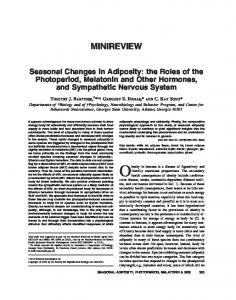
range of speech intensities at each frequency that contribute to the understanding of the speech signal . Olsen et al (1987) have recently reviewed a wide variety of "speech audiograms" and conclude that the one from Pascoe shown in Figure 1 is one of the most appropriate to use because of the unique manner in which it was derived. Pascoe (1980) filtered 1/3-octave bands from a speech sample and measured the thresholds for detection of these bands in a group of normal-hearing subjects . The sound pressure level of each band at threshold represented 0 dB sensation level for the speech signal or 0 dB HL since a group of normal listeners were used. By then presenting the speech at normal conversational levels, acoustically measuring the 1/3-octave levels for this signal, and referencing them to the measured detection thresholds, the levels of each 1/3-octave band in dB HL could be established. The letters included on the speech audiogram in Figure 1 are orthographic representations of various speech sounds . They have been distributed along the audiogram according to their relative intensities and spectral content in a manner not unlike that suggested by Tyler (1979) . This type of audiogram format can be valuable as a tool to explain the effects of hearing loss on speech understanding. Consider a lisFrequency in Hz 125

250

500

1000

2000

4000

8000

0) 00

"SPEECH AUDIOGRAW igure 1 illustrates the "speech audiogram" Fthat will be used frequently to illustrate how simply prediction or estimation of speechrecognition performance can be made . The solid and dashed lines in this particular speech audiogram are taken from Pascoe (1980) . The solid line represents the average intensity of a conversational speech signal presented at an overall sound pressure level of 65 dB . The upper and lower dashed lines represent the 60

Figure 1 Illustration of the "speech audiogram" used throughout much of this paper. The solid line represents the root-mean-square (rms) sound levels, in dB HL, for a speech signal having an overall sound pressure level of 65 dB . The dashed lines represent the range of speech levels that fluctuate about the rms levels from moment to moment. Orthographic representations of various speech sounds have been superimposed on the speech audiogram to illustrate their relative amplitudes and frequency content.

Speech Understanding/Humes

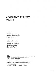
tener with a sloping high-frequency sensorineural hearing loss . When this listener's hearing thresholds are plotted on the speech audiogram shown in Figure 1, an explanation for the common complaint, "I can hear speech, but I can't understand it," is immediately apparent to the clinician and, more importantly, the patient. The concept of a speech audiogram is not new. Olsen et al (1987), for example, trace the origins of the concept to 1928 . What is new, however, is the recognition that most of the speech-understanding problems of the hearing impaired can be explained by such a simple scheme . For years, audiologists and hearing scientists have been searching for other peripheral and central-processing deficits that might explain the difficulty experienced by the hearing impaired on a number of speech-recognition tasks. In the mid 1980s, for example, the hearing loss of the listener was considered to have only a relatively minor influence on speech-recognition scores obtained in noise, with deficits in spectral and temporal resolution playing a major role (Dreschler and Plomp, 1980,1985; Festen and Plomp,1983 ; Preminger and Wiley, 1985 ; Stelmachowicz et al, 1985) . Recent research efforts, however, are converging on the same conclusion ; the primary factor responsible for the speech-recognition problems of the hearing-impaired in quiet and in noise is the loss of hearing sensitivity and accompanying loudness recruitment. This conclusion manifests itself in data collected on the application of the Articulation Index to the hearing impaired (Pavlovic, 1984 ; Kamm et al, 1985 ; Dirks et al, 1986 ; Humes et al, 1986 ; Pavlovic et a1,1986; Dubno et a1,1989), on the simulation of the psychoacoustic performance of the hearing impaired by noise-masked normals (Jesteadt et al, 1987 ; Humes et al, 1988 ; Dubno and Schaefer, 1989), and on the simulation of the speech-recognition performance of the hearing impaired by noise-masked normal listeners (Fabry and Van Tasell,1986; Humes et a1,1987; Zurek and Delhorne, 1987). The top panel of Figure 2 shows the same speech audiogram, but with the orthographic symbols representing individual speech sounds removed. It is clear that the normal-hearing listener has the full range of speech intensities audible from 250 through 8000 Hz for a conversational speech signal in quiet. In the bottom panel, a similar representation has been provided for a white noise masker delivered at an

Frequency in Hz 125

250

500

1000

2000

4000 8000

Frequency in Hz -10 0000 o'

125

250

500

1000 2000

4000

8000

0 10

White Noise OASPL = 65 dB Figure 2 Illustration of the speech audiogram from Figure 1, but with the speech sounds removed. The top panel illustrates a quiet listening condition for a normal listener whereas the bottom panel displays speech in a background of white noise . The masking spectrum of the white noise, in dB HL, is shown as a dotted line . With both speech and noise at 65 dB SPL, this represents a signal-to-noise ratio of 0 dB .

overall level of 65 dB SPL. The dotted line represents the masked thresholds predicted for such a noise stimulus . In the presence of this white-noise background, speech intensities below the dotted line will not be audible to the normal listener and speech understanding decreases. As the level of the noise is increased or decreased the dotted lines would be raised or lowered on the speech audiogram. Essentially, as the amount of the speech signal masked by the noise increases, speech understanding decreases. Now consider a moderate sloping high-frequency sensorineural hearing loss like the one

Journal of the American Academy of Audiology/Volume 2, Number 2, April 1991

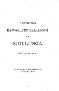
shown in Figure 3. The top panel represents the situation for speech presented at 65 dB SPL in quiet, whereas the bottom panel depicts the case of speech presented in a background of white noise (65 dB SPL, 0-dB signal-to-noise ratio). In the top panel, note that much of the speech signal falls below threshold, resulting in reduced speech understanding. Although this hypothetical listener hears speech, especially lower frequency vowels and consonants (see Fig. 1), the inaudibility of the high-frequency speech sounds results in a deficit in speech understanding. In this particular case, adding a background of white noise at a 0-dB speech-tonoise ratio results in little change in speech understanding. That is, there is little masking produced by the noise such that the quiet Frequency in Hz 125

250

500

1000

2000 4000

8000

"-" Sloping SNHL

Frequency in Hz 125

250

500

1000

2000

4000 8000

m 00

"-" Sloping SNHL White noise--65 dB Figure 3 Same as Figure 2, but for a listener with a sloping high-frequency sensorineural hearing loss . Notice in the bottom panel that the noise is barely audible and does not reduce the audible portion of the speech signal appreciably.

62

thresholds of the hearing-impaired listener are still the primary limiter of speech understanding . Note, moreover, that little of the noise is actually audible to the hearing-impaired listener and that the portion of the speech signal that is above threshold in noise is very similar for the hearing-impaired person and the normal listener (bottom panel of Fig. 2) . Thus, the speech-understanding deficit experienced by the hearing-impaired listener, relative to performance of the normal listener, is much greater in quiet (top panels of Figs . 2 and 3) than in noise (bottom panels of Figs . 2 and 3) . Figure 4 illustrates the situation for amplified or aided speech signals. For this analysis, it has been assumed that the gain prescribed by the POGO method (McCandless and Lyregaard, 1983) has been realized on the patient and that both speech and noise are amplified the same amount. Rather than plot improved thresholds for the aided condition (functional gain) and leaving the speech spectrum unaltered, the speech and noise spectra have been amplified by an amount corresponding to the prescribed gain . Comparison of the top panel of Figure 4 with the corresponding panel of Figure 3 reveals that much more of the speech signal is now audible for the aided listening condition in quiet. Note, however, that even under the assumption of an optimal match between prescribed and obtained gain, the entire range of speech intensities important for intelligibility is not audible for the aided speech signal . This is especially true for the high frequencies . Moreover, the actual insertion gain obtained in the high frequencies is frequently 10-20 dB lower than that prescribed (Cox and Alexander, 1990 ; Humes and Hackett, 1990). This would result in even less speech intensity being amplified above threshold than shown in Figure 4. In the bottom panel of Figure 4, note that the noise (dotted line) has also been amplified by the hearing aid so that now the noise, rather than the quiet thresholds, becomes the factor limiting the audibility of the speech signal . Two points are noteworthy regarding the bottom panel of Figure 4. First, the noise that was inaudible without the aid is now audible, and probably annoying, to the listener, unlike the unaided situation (Fig. 3, bottom) . Second, the audible portion of the speech signal has increased only slightly from unaided to aided listening and is limited by the amount audible to a normal-hearing listener . That is, the audible area of the speech signal in the

Speech Understanding/Humes

bottom panel of Figure 4 is identical to that in the bottom panel of Figure 2. If the normal listener understands only 60 percent of the speech materials for the 0 dB speech-to-noise ratio represented in the bottom panel, then the hearing-impaired listener can not exceed that level of performance unless the speech-to-noise ratio is improved in some manner (directional microphones, FM or infrared systems, signal processing, etc. ). So, as a result of amplification, the hearing-impaired listener represented in Figures 3 and 4 understands speech much better in quiet, only slightly better in noise (and no better than a normal listener under those same conditions), and is likely to complain about the audibility of "noises" not heard prior to amplification. This common clinical scenario is explained quite nicely by the speech audiogram . The explanatory power of the speech audiogram is not restricted just to sloping losses or understanding of aided versus unaided speech recognition . It has been noted frequently, for example, that hearing-impaired listeners have much greater difficulty understanding speech in low-pass noise than in broad-band noise ( Cohen and Keith, 1976 ; Keith and Talis, 1976 ; Stelmachowicz et al, 1985, 1990). This has been quantified in several ways, but most of the recent data have been obtained using adaptive estimates of the speech-to-noise ratio needed for a criterion performance level, usually 50 percent correct (e .g., Stelmachowicz et al, 1990). The top two panels of Figure 5 illustrate the speech audiogram for normal listeners listening to conversational speech in backgrounds of white noise (left panel) and low-pass noise (right panel) . The estimated masking produced by the two noise spectra is shown by the dotted lines in each panel. The overall level of both noise maskers is fixed at 65 dB SPL in this example. Note that more of the speech spectrum is audible in the right panel than in the left . To equate the audible portions of the speech spectrum and thereby produce equal levels of performance, the level of the low-pass noise would need to be increased or the level of the white noise decreased. In either case, normal listeners would require a more favorable speech -to-noise ratio in white noise to achieve the same level of performance as in low-pass noise. The remaining four panels in Figure 5 depict the speech audiograms for two hypothetical hearing-impaired listeners. Although they both have pure-tone averages of 40 dB, the mid-

Frequency in Hz 125

0) 00

1

250

500

1000

2000 4000 8000

"-" Sloping SNHL AIDED--POGO

125

Frequency in Hz

250

500

1000 2000

4000 8000

0) 00 0)

\-_i

"-" Sloping SNHL AIDED--POGO; White Noise Figure 4 Illustration of amplified speech and noise for a hearing aid with gain characteristics set according to the POGO prescriptive method. Top panel illustrates speech in quiet, whereas the bottom panel illustrates speech in noise. Compared to Figure 3, much more of the speech signal is audible in quiet (top panel) with amplification, but only slightly more is audible in noise (bottom panel) . Much more of the noise, however, is audible in the aided condition than in the unaided condition (Fig . 3) .

dle two panels depict a sloping high-frequency sensorineural hearing loss, whereas the bottom two panels represent an individual with a flat loss . The noise levels and masking spectra are identical to those shown in the top two panels for a 0-dB speech-to-noise ratio. In the middle panels, note that the low-pass noise (right panel) reduces the portion of the speech spectrum audible to this hypothetical listener more than the white noise (left panel). Thus, for this listener with sloping loss, the low-pass noise would need to be reduced or the white noise increased to produce equivalent perfor-

Journal of the American Academy of Audiology/Volume 2, Number 2, April 1991

Figure 5 The speech audiogram is used here to illustrate the relative speech-understanding difficulties encountered by white noise (left panels) and low-pass noise (right panels) . The overall sound pressure levels of the noises are the same in all panels (65 dB SPL, or 0 dB signal-to-noise ratio). The top two panels represent a listener with normal hearing (0 dB HL), the middle two panels represent a sloping sensorineural hearing loss (PTA = 40 dB HL), and the bottom two panels represent a flat sensorineural hearing loss (PTA = 40 dB HL).

-10

0m

D 10

125

Frequency in Hz

250

1

500 1000 2000 4000 8000

125

Frequency in Hz

250

500 1000 2000 4000 8000

N

White Noise OASPL = 65 dB

125

Frequency in Hz

250

500

1000 2DOO 4000 8000

"-" Sloping SNHL White noise--65 dB

Frequency in Hz 125 250 500 1000 2000 4000 BOW

0- " Sloping SNHL Low-Pass Noise

Frequency in Hz 125

250

500 1000 2000 4000 8000

125

Frequency in Hz

250

500 1000 2000 4000 8000

"-" Flat SNHL Low-Pass Noise

mance. In addition, when compared to the normal listener in the top two panels, the high-frequency hearing-impaired listener would require a more favorable speech-to-noise ratio for low-pass noise and, to a lesser extent, for white noise. Inspection of the speech audiograms in the bottom two panels for the flat sensorineural hearing loss reveals that the masking noise, though slightly audible, results in little reduction in the audible portion of the speech spectrum and, therefore, speech-recognition performance. The speech-to-noise ratio required by the normal listeners (top panels) for the same level of performance as for the listeners with flat sensorineural hearing loss (bottom panels) would be much poorer . That is, the noise level would have to be increased con64

siderably in the normal listeners, especially for the low-pass noise, to reduce the audible portion of the speech spectrum by the same amount as for the listeners with flat loss . The speech audiograms in Figure 5, therefore, indicate that the hearing-impaired listeners with sloping and flat audiometric configurations require more favorable speech-tonoise ratios than normal listeners for the same level of speech-recognition performance. This is a common finding in the numerous studies using such a paradigm (see Plomp, 1978, 1986 for reviews) . In addition, a much more favorable speech-to-noise ratio is required in low-pass noise for the hearing-impaired listeners than for the normal listeners whereas only a slight improvement in speech-to-noise ratio is required in

Speech Understanding/Humes

white noise. This differential effect has led others to speculate about "excessive upward spread of masking" in the hearing impaired (e .g ., Stelmachowicz et al, 1985, 1990). In the present simplified "speech audiogram" approach, however, this differential effect oflow-pass noise and white noise is predicted independently of possible abnormal masking effects. Careful consideration of the "speech audiogram" can explain many of the speech-recognition difficulties of the hearing impaired . Consideration of the distribution of speech sounds within the speech spectrum (Fig . 1) can assist in understanding the nature of the listener's misperceptions . The speech audiogram can also provide a qualitative explanation of the limitations of conventional linear amplification and of the differential effects of different types ofnoise maskers . In many instances, such as counseling, teaching, and internalizing conceptual frameworks, qualitative explanations are sufficient . Many applications, however, could make better use of quantified predictions from the speech audiogram . The Articulation Index (AI) represents one form of speech audiogram quantification. The Al has been a useful tool for estimating the benefit of amplification (Pavlovic, 1988), the "greaterthan-expected" speech-understanding difficulties of some elderly listeners (Kamm et al, 1985 ; Schum et al, in press), and even the effects of hearing protection on the speech-understanding of listeners with noise-induced hearing loss (Wilde and Humes,1990). Essentially, the AI assigns a number from 0 to 1 .0 that represents the proportion of the speech signal audible to the listener in quiet and noisy listening situations . Two clinical versions of the Al are reviewed and evaluated in the next section .

125

avlovic (1988, 1989) has described an AIPcalculation scheme based on a simplified speech audiogram. His representation of the speech audiogram for this purpose is shown in Figure 6 . The striped region in this figure schematically represents the same region represented by the dashed lines in Figures 1 through 5. Because of the relatively minor contributions to speech-recognition made by the lowest and highest frequencies on the audiogram, Pavlovic (1988, 1989) has eliminated the speech spectrum below 500 Hz and above 4000

FREQUENCY IN Hz 500 1000 2000

F

4000

P

8000

m

P

Figure 6 Al audiogram from Pavlovic (1988). The striped area in this figure corresponds to the region between the dashed lines in the previous figures; that is, the usable ranges of speech intensities from peak level (p) to minimum level (m). This Al scheme is referred to here as the equally weighted Al .

Hz . The remaining four frequencies, 500, 1000, 2000, and 4000 Hz, are all assumed to contribute equally to speech recognition . Note that there is a 30-dB range for the speech spectrum at each of these frequencies, from 20 to 50 dB HL . If we sum this 30-dB range of speech intensities at each of the four frequencies, the result is 120 dB . To calculate the AI in this approach, one simply determines how many dB of the speech spectrum are audible at each of the four frequencies, sums the four dB values, and divides by the maximum possible (120). A Frequency in Hz -10 m 00 Q)

0

10

125

250

500

1000 2000

4000

8000

. . .. . . . . . . . . .. . . .. ./. .. . . .

20 30

ARTICULATION-INDEXAUDIOGRAM

250

m a)

Q)

J C

'C 0

_r

40

: . . .x . . .40 .

.

"

"

50

60 70 90

90

100 110

Figure 7 Al audiogram modified from Cavanaugh et al (1962) . Dashed lines are as in Figures 1-5. The dots at each frequency contribute 0.03 toward the Al and reflect the relative contribution of various frequency regions to the Al . This Al calculation scheme is referred to here as the high-frequency weighted Al .

65

Journal of the American Academy of Audiology/Volume 2, Number 2, April 1991

normal-hearing listener with thresholds of 0 dB HL at all frequencies would have the full speech spectrum audible, or (30+30+30+30 dB)/120 dB . This reduces to 120/120 or an AI of 1 .0 . A flat hearing loss of 40 dB superimposed on the speech audiogram in Figure 6 would result in an AI of 0.33 ((10+10+10+10)/120). This AI approach is applied to aided situations by simply increasing the shaded speechspectrum area by the amount of real-ear gain measured at each frequency. Pavlovic (1988,1989) assumed that each frequency included in the calculations contributes equally to speech recognition (that is, the 30-dB speech range at 500 Hz is "worth" the same as the 30 dB at 2000 Hz, as far as speech recognition is concerned). This assumption is not universally accepted. The current ANSI standard for the calculation of the AI, ANSI S3 .5-1969, for instance, assigns much greater weight to 2000 Hz than to 500 Hz . An alternative AI audiogram that incorporates weighting factors consistent with the ANSI standard appears in Figure 7 . This AI audiogram was developed by the author and is a modification of a similar concept applied in architectural acoustics by Cavanaugh et al (1962). In this approach, one simply counts the number of dots above threshold and multiplies by 0.03. Each dot, therefore, contributes 0.03 to the AI . There are more dots within the 30-dB range of the speech spectrum at 2000 and 4000 Hz than at the other frequencies, reflecting the greater importance of these frequencies to speech recognition . The dashed lines in this figure represent the range of speech intensities at each frequency and are identical to those shown previously in Figures 1 through 5 . In this particular AI audiogram, aided results are calculated by improving the hearing thresholds by the amount of real-ear gain measured . The two clinical AI calculation schemes, referred to here as the equal-weight AI (Fig . 6) and the high-frequency weighted AI (Fig . 7), were evaluated using the speech-recognition scores from a group of 12 listeners with moderately sloping sensorineural hearing loss who had participated in a previous study (Humes and Hackett, 1990). Each of the 12 listeners in that study was tested in quiet, using the CUNY Nonsense Syllable Test (Resnick et al, 1975), for aided and unaided listening conditions . The rms speech level for the NST materials was 70 dB SPL, rather than the 63 and 65 dB SPL levels assumed by the equally weighted and high-frequepcy weighted AI calculation schemes, respec66

1 .0

z 0 0 a_ o

" CD O ®O . O 0.4

"

40 " Unaided I O Aided

0 .2 0.0 0 .0 1 .0

0 .0 0.0

NST in Quiet 0.2

0 .4

0 .6

0.2

0.4

0 .6

0.8

1 .0

0.8 EQUALLY WEIGHTED AI

1 .0

HIGH-FREQUENCY WEIGHTED AI

Figure 8 Scatterplots of the proportion correct on the CUNY NST as a function of the Al for the high-frequency weighted Al (top panel) and the equally weighted Al (bottom panel) . Filled circles represent unaided performance and open circles represent aided performance for 12 listeners with sensorineural hearing loss tested previously by Humes and Hackett (1990) .

tively . Consequently, the speech levels in Figures 6 and 7 were adjusted accordingly prior to AI calculation . Each subject had one unaided score and three aided scores, one aided score for each of three different BTE hearing aids . Measures of real-ear gain in the aided listening conditions were obtained using probe-tube microphones . The scattergrams of speech-recognition score by AI for each of the clinical Al calculation schemes are shown in Figure 8. The filled symbols represent unaided performance, whereas the unfilled symbols represent aided scores . Both the aided and unaided scores increase as the AI increases for both calculation schemes. The correlation between unaided speech-recog-

Speech Understanding/Humes

Table 1 Pearson-r Correlation Coefficients between NST Score and Al for Each Subject across Four Listening Conditions for Each of the Al Calculation Methods Subject 01 02 03 04 05 06 07 08 09 10 11 12

Equally Weighted Al 0 .96 0 .96 0 .99 0 .46 0 .97 -0 .25 0 .77 0 .97 0 .84 -0 .28 0 .95 0 .90

High-FrequencyAl 0 .96 0 .99 0 .99 0 .39 0 .98 -0 .32 0 .73 0 .96 0 .83 -0 .39 0 .94 0 .97

nition score and the AI was 0.93 and 0.91 for the high-frequency weighted and equally weighted versions of the AI, respectively. For the aided conditions, however, the equally weighted version of the AI fared slightly better than the high-frequency weighted version with correlation coefficients of 0.75 versus 0.73 . The correlation between the two clinical AI values, moreover, was 0.97 for both aided and unaided conditions . Thus, both clinical Al methods are closely related, despite differences in weighting factors, and both can describe unaided performance with a high degree of accuracy, but aided performance with only moderate precision. It is clear from Figure 8 that the aided and unaided speech-recognition scores fall into two different clusters with the aided conditions consistently yielding lower scores than the unaided conditions for the same AI value. This is particularly evident for 0.6 < AI < 0.8 . It may not be possible to predict precisely the aided performance of the hearing impaired by considering only the amount of gain at each frequency, as is the case with both clinical AI calculation schemes. Performance in the aided conditions may be decreased by factors not considered in this simple scheme, such as the distortion and internal noise introduced by the hearing aid. Aside from providing comparisons of how hearing-impaired listeners perform relative to normal listeners, another suggested application of the AI involves the relative comparison of performance across aids or conditions within a given listener . That is, can the AI be used to rank/order different hearing aids for a par-

ticular patient with respect to speech-recognition performance? If so, then the correlations of NST scores with the calculated AI values across aids and conditions (aided versus unaided) should be strong and positive . The correlations for each of the 12 subjects (4 scores/subject) and each Al calculation method are shown in Table 1 . In general, the correlations indicate that as the AI increased, the NST score also increased . Three clear exceptions, however, are subjects 4, 6, and 10, two of whom have slightly negative correlations between NST score and AI . These same three subjects, however, had the three highest unaided NST scores in quiet (94%, 89%, and 86%) . This resulted in an extremely narrow range of scores across the four conditions for each of these subjects and resulted in very low correlations . In general, the correlations in Table 1 support the use of these two clinical versions of the Al as relative predictors of speech-recognition performance for aided listening in quiet .

SUMAURY he present tutorial has demonstrated that T many of the speech-understanding problems of the hearing impaired can be understood qualitatively using the "speech audiogram" or quantitatively using the Articulation Index . There are

limitations, however, to both approaches that must be understood . For example, it has been noted since the inception of the Al model, that the AI only predicts or estimates the overall speechrecognition score and does not indicate the types of errors that are being made (Fletcher and Galt, 1950) . Two listeners with AIs of 0 .4 and predicted word-recognition scores of 67 percent may have completely different patterns of errors .

Consider also the application of the AI to aided listening conditions . Without any restrictions at high intensities, one might suggest that the AI can be maximized by simply giving every listener 100 dB of gain at all frequencies! This is obviously not possible or desirable. Most AI calculation schemes, however, have some means of reducing the contribution of high-intensity speech signals to speech recognition, thereby limiting the amount of benefit received from excessive amounts of gain (e .g, ANSI, 1969 ; Pavlovic, 1989). Finally, the AI cannot accurately predict the disproportionate loss of speech understanding observed in many elderly hearing-impaired listeners (Kamm et al, 1985 ; Schum et al, in press) . 67

Journal of the American Academy of Audiology/Volume 2, Number 2, April 1991

However, as noted previously, the AI can be used with such listeners at least to identify those who are having "greater-than-expected" difficulties understanding speech. By doing so, those patients identified in this manner could be counseled appropriately about the limited benefit of amplification and targeted for additional rehabilitative procedures . Acknowledgments. This work was supported, in part, by grants from NIDCD and NIA.

REFERENCES American National Standards Institute. (1969) . Methods for the Calculation of the Articulation Index. ANSI S3 .51969 . NewYork: American National Standards Institute. Burney PA . (1972) . A survey of hearing aid evaluation procedures . Asha 14 :439-444 .

Humes LE, Hackett T. (1990) . Comparison of frequency response and aided speech-recognition performance for hearing aids selected by three different prescriptive methods. JAmAcad Audiol 1:101-108 . Humes LE, Dirks DD, Bell TS, Ahlstrom C, Kincaid GE . (1986) . Application of the articulation index and the speech transmission index to the recognition of speech by normal-hearing and hearing-impaired listeners . J Speech Hear Res29:447-462 . Humes LE, Dirks DD, Bell TS, Kincaid GE . (1987) . Recognition of nonsense syllables by hearing-impaired listeners and by noise-masked normal hearers. JAcoust Soc Am 81 :765-773 . Humes LE, Espinoza-Varas B, Watson CS . (1988) . Modeling sensorineural hearing loss . 1. Model and retrospective evaluation . JAcoust Soc Am 83 :188-202 . Jerger J. (1987) . On the evaluation of hearing aid performance. Asha 29(9):49-51 . Jesteadt W, Stelmachowicz PG, Callaghan BP . (1987) . Predicting masked thresholds in impaired listeners from combinations of normal masked thresholds and hearing loss . JAcoust Soc Am 81(Sl) :S77 .

Carhart R. (1946) . Selection of hearing aids . Arch Otolaryngol 44 :1-18 .

Kamm C, Dirks DD, Bell TS . (1985). Speech recognition and the articulation index for normal and hearing-impaired listeners. JAcoust Soc Am 77 :281-288 .

Cavanaugh WJ, Farrell WR, Hirtle PW, Walters GB . (1962) . Speech privacy in buildings. J Acoust Soc Am 34 :475-492 .

Keith RW, Talis H. (1976) . The effects of white noise on PB scores of normal and hearing-impaired listeners . Audiology 11 :177-186 .

Cohen RL, Keith RW . (1976) . Use of low-pass noise in word recognition testing. J Speech Hear Res 19 :48-54 .

Martin FN, Morris LJ . (1989) . Current audiologic practices in the United States . Hear J 4 :25-44 .

Cox RM, Alexander GC . (1990) . Evaluation of an in situ output probe-microphone method for hearing aid fitting verification . Ear Hear 11 :31-39 .

McCandless GA, Lyregaard PE . (1983) . Prescription of gain/output (POGO) for hearing aids . Hear Instr 34(1) :16-21 .

Dirks DD, Bell TS, Rossman RN, Kincaid GE . (1986). Articulation index predictions of contextually dependent words. JAcoust Soc Am 80 :82-92 .

Olsen WO, Hawkins DB, Van Tasell DJ . (1987). Representations of the long-term spectra of speech. Ear Hear 8:1008-108S .

Dreschler WA, Plomp R. (1980) . Relation between psychophysical data and speech perception for hearingimpaired subjects . 1. JAcoust Soc Am 68 :1608-1615 .

Pascoe DP . (1980) . Clinical implications of nonverbal methods of hearing aid selection and fitting . SemSpeech Lang Hear 1:217-229 .

Dreschler WA, Plomp R. (1985) . Relations between psychophysical data and speech perception for hearingimpaired subjects . 11 . JAcoust Soc Am 78 :1261-1270.

Pavlovic CV . (1984) . Use of the articulation index for assessing residual auditory function in listeners with sensorineural hearing impairment . J Acoust Soc Am 75:1253-1258 .

Dubno JR, Schaefer AB . (1989) . Frequency resolution for broadband-noise masked normal listeners. JAcoust Soc Am 86(Sl):S122. Dubno JR, Dirks DD, Schaefer AB . (1989) . Stop-consonant recognition for normal-hearing listeners and listeners with high-frequency hearing loss . II : Articulation index predictions . JAcoust Soc Am 85 :355-364 . Egan JP . (1948) . Articulation testing method . Laryngoscope 58 :955-991 . Fabry DA, Van Tasell DJ . (1986) . Masked and filtered simulation of hearing loss : effects on consonant recognition . J Speech Hear Res 29 :135-141 . Festen JM, Plomp R. (1983) . Relations between auditory functions in impaired hearing. JAcoust Soc Am 73 :652662. Fletcher H, Galt RH . (1950) . The perception of speech and its relation to telephony. JAcoust SocAm 22 :89-151. Humes LE . (1988) . And the winner is . . . Hear Instr 7:2426 .

68

Pavlovic CV . (1988) . Articulation index predictions of speech intelligibility in hearing aid selection . Asha 30(6):63-65 . Pavlovic CV . (1989) . Speech spectrum considerations and speech intelligibility predictions in hearing aid evaluations. J Speech Hear Disord 54 :3-8 . Pavlovic CV, Studebaker GA, Sherbecoe RL . (1986) . An articulation index based procedure for predicting the speech recognition performance of hearing-impaired individuals. J Acoust Soc Am 80 :50-57 . Plomp R. (1978) . Auditory handicap of hearing impairment and the limited benefit of hearing aids . JAcoust Soc Am 63 :533-549 . Plomp R. (1986) . A signal-to-noise ratio model for the speech-reception threshold of the hearing impaired . J Speech Hear Res29:146-154. PremingerJ, Wiley TL. (1985) . Frequency selectivity and consonant intelligibility in sensorineural hearing loss . J Speech Hear Res28:197-206.

Speech Understanding/Humes

Resnick DM, Becker M. (1963) . Hearing aid evaluation: a new approach . Asha 5:695-699 . Resnick S, Dubno JR, Hoffnung S, Levitt H. (1975) . Phoneme errors on a nonsense syllable test . JAcoust Soc Am 58(Suppl . 1) :S114. Schum DJ, Matthews LJ, Lee FS . (In press). Actual and predicted word recognition performance of elderly, hearing-impaired listeners. J Speech Hear Res. Shore I, Bilger RC, Hirsh 1. (1960). Hearing aid selection for severe to profound hearing loss . JSpeech HearDisord 25 :152-167 . SmaldinoJ, HoeneJ . (1981a). Aview of the state ofhearing aid fitting practices. Part 1. Hear Instr 32(1):14-15, 58 . Smaldino J, Hoene J. (1981b). The nature ofcommon hearing aid fitting practices. Part 11 . Hear Instr 32(2):8-11, 43 . Stelmachowicz PG, Jesteadt W, Gorga MP, Mott J. (1985) . Speech perception ability and psychophysical tuning curves in hearing-impaired listeners . JAcoust Soc Am 77 :620-627 .

Stelmachowicz PG, Lewis DE, Kelly WJ, Jesteadt W. (1990) . Speech perception in low-pass filtered noise for normal and hearing-impaired listeners. J Speech Hear Res 33 :290-297 . Tyler R. (1979) . Measuring hearing loss in the future . Br JAudiol (Suppl. 2) :29-40. Walden BE, Schwartz DM, Williams DL, Holum-Hardegen LL, Crowley JM . (1983) . Test of the assumptions underlying comparative hearing aid evaluations . J Speech Hear Res 21 :507-518 . Wilde G, Humes LE . (1990) . Application of the articulation index to the speech recognition of normal and impaired listeners wearing hearing protection . JAcoust Soc Am 87 :1192-1199 . Zurek PM, Delhorne LA . (1987) . Consonant reception in noise by listeners with mild and moderate sensorineural hearing impairment. JAcoust Soc Am 82 :1548-1559 .