of musical structure that captures local prediction and global rep- etition properties of audio ...... by musical ensemble, such as for the case of orchestral music.
1
Unified View of Prediction and Repetition Structure in Audio Signals with Application to Interest Point Detection Shlomo Dubnov University of California, San Diego
Abstract— In this paper we present a new method for analysis of musical structure that captures local prediction and global repetition properties of audio signals in one information processing framework. The method is motivated by a recent work in music perception where machine features were shown to correspond to human judgments of familiarity and emotional force when listening to music. Using a notion of information rate in a modelbased framework, we develop a measure of mutual information between past and present in a time signal and show that it consist of two factors - prediction property related to data statistics within an individual block of signal features, and repetition property based on differences in model likelihood across blocks. The first factor, when applied to spectral representation of audio signals, is known as Spectral Anticipation, and the second factor is known as Recurrence Analysis. We present algorithms for estimation of these measures and create a visualization that displays their temporal structure in musical recordings. Considering these features as a measure of the amount of information processing that a listening system performs on a signal, information rate is used to detect interest points in music. Several musical works with different performances are analyzed in the paper, and their structure and interest points are displayed and discussed. Extensions of this approach towards a general framework of characterizing machine listening experience are suggested. Index Terms— Spectral Anticipation, Recurrence Matrix, Information Rate, Spectral Clustering, Musical Structure, Visualization, Interest Points
I. I NTRODUCTION The concept of anticipation seems to have been attracting recently a lot of attention in musical research [1],[2],[3],[4]. The importance of the topic has been long-time acknowledged, considering expectations as one of the major factors in shaping musical listening experience [5],[6]. The apparently intuitive link between successes and failures of expectations and emotional responses seem to require little justification. According to Meyer [6], listeners constantly develop perceptual expectancies about the possible evolution of the music, with emotions arising from the way the composer fulfills or frustrates these expectancies. Following this foundation of a cognitive approach to music perception, the processes of expectancy and anticipation have been investigated in music cognition, usually in terms of specific musical parameters such as melody, harmony, tonality and rhythm [7],[8],[9]. Other studies investigate relations between expectancies and neural correlates [10],[11], showing for instance commonalities with networks previously described for target detection and novelty
processing. Both the strengths and weakness of these studies are in that they are dealing with models of human perception in specific musical terms. Moreover, they usually employ synthetic examples of limited musical complexity or naturaleness and rely on musical knowledge in order to correlate musical structure to listener responses. The method presented in this paper works directly from digital audio, without assuming any musical knowledge. We employ information theoretic methods to construct an anticipation measure of spectral observations, which in principle can be applied to any structured audio signal. It should be acknowledged that information theoretic approaches had been advocated in such early works as Moles [12] and Meyer [6]. It is important to note that these approaches usually convey measures of complexity or uncertainty (entropy) in music, rather then predictive success of a listening system. This point is discussed at length by Huron in his book [2]. In a recent work [13] we suggested new features that characterize structural and affective aspects of music from statistical audio signal analysis in attempt to approximate human reactions of familiarity and emotional force that were collected in listening experiments. The idea in that work was twofold: first we assumed that the act of listening to a complex audio signal must involve certain types of mental processing, which should have parallels in terms of computational tasks such as classification, clustering or prediction. Secondly, we assumed that these high level cognitive responses, namely emotional force and familiarity, would be related to self-appraisal of the successes and failures of these mental faculties. Accordingly, we introduced an anticipatory information rate measure [3] that is based on computation of prediction gain of coefficients in spectral or audio-basis representations of audio signals, such as sound effects or musical recordings. When run on non-stationary and time varying data such as music, the changes in information rate correlate well with human emotional force data, resulting in what we called ”spectral anticipatory profile”, or in short ”spectral anticipation”. The global properties of the audio data were analyzed in terms of recurrence properties of the time-varying spectral frames. By using eigen-analysis [14] of the signal recurrence (self-similarity) matrix1 [15] we created a ”spectral recurrence profile” that matched or ”explained” significant portions of the 1 Methods of applying eigenvector analysis to matrices that contain pairwise data similarity values are also known as ”spectral clustering”.
2
human familiarity curve. In this paper we present a unified view of anticipation by using parametrization of the audio feature distribution function. We show that the information carried by a signal over time is actually a combination of information rate within the current model, and the cost associated with the likelihood of observing this model under some probability distribution over the model space. In other words, we generalize the Spectral Anticipation method for the case of parametric processes so that it correctly includes a factor related to model changes across frames, which can be approximated by Recurrence Profile. We show that only when combined together, these profiles measure the overall amount of mutual information that past data carries about the present. In terms of musical significance, the two measures, namely the anticipatory and recurrence profiles, capture complementary intra- and interblock statistical properties of the data. The new approach combines the original spectral anticipation and spectral recurrence measures of [13] under a single formalism, thus unifying the two information bearing properties of the data. We suggest a method for visualization of the two measures in a manner that allows a convenient eyeballing of these two aspects of signal structure. Motivated by cognitive interpretations of these features, we claim that the proposed visualization method captures some of the global memory (inter-) and local (intra-block) excitation structure of the audio signal. Accordingly, we termed these displays as ”Memory and EXcitation”, or MEX patterns. The patterns allow for a visual representation of the overall structure in terms of how typical the spectral contents are, grading them from typical to rare, and for a visual representation of the local structure in terms of prediction-gain properties of short sequences of spectral parameters. As will be explained below, the likelihood of certain musical material is related to the amount of ”surprise” on the level of musical form. On the immediate, intra-block level, low values of prediction gain occur in the cases of both purely random or constant signals, indicating that both types of materials are ”not interesting” for musical purposes, while high gain occurs for signals that have large variation in their parameters, but whose dynamics can be predicted and thus uncertainty can be significantly reduced by such prediction. On the overall one might conclude that the information contents occurring in music over time are a combination of two factors - surprise related to musical form and surprise or excitement related to musical texture characteristics. The paper is organized as follows - first we discuss the concept of anticipation and present mathematical formalization in terms of mutual information between past and present that we call information rate (IR). Assuming a parametric distribution, IR is further developed as a combination of two factors, intrablock or data-IR, and inter-block or model-IR. Algorithms for estimation of data-IR and model-IR are presented next, using an independent components approximation in the case of intrablock analysis, and Markov approximation for modeling of the inter-block statistics. Finally, we explain the method of visualizing the two measures (data- and model-IR) and test it on several musical examples containing different performances of three piano pieces. Our choice of musical examples was
done in a manner that allowed for different aspects of the MEX patterns to be qualitatively evaluated. For one, all our examples were drawn from solo piano repertoire, making these signals difficult to analyze since they are polyphonic and monotimbral. The choice of piano works from different composers and genres, namely Bach Prelude from Well Tempered Clavier (Prelude number 2 in C minor, Book I), Chopin’s “Minute Waltz” and Beethoven “For Elise”, was done so as to examine MEX on different types of musical materials in terms of form and texture. We analyzed different interpretations, including one synthetic rendering, to demonstrate the range of variations that MEX patterns have across pieces and performances. In the last part of the paper we use MEX patterns to detect points of maximal interest in music, with a detailed analysis of Bach Prelude. II. A NTICIPATION -
FORMALLY DEFINED
Prediction is an act of forecasting, or an attempt in making the result known before hand. Anticipation is an action that a system takes as a result of prediction, including its ability to alter its internal state (behavior or feelings) according to results of prediction. In order to function, such system has to consider the errors that occur between its predictions and the actual outcomes, performing an appraisal of its own functioning. If the signal appears complex a-priori, but its uncertainty is greatly reduced after prediction, then anticipation has achieved its goal. If the signal is either constant or random, which means that it can not be predicted, then the role of anticipation is minor. By averaging over multiple signal and prediction error instances, we shall define an anticipation measure as the difference in uncertainty that a system has with respect to data, before and after performing prediction. Since we are dealing with temporal processes, we shall view the actions of a listening system as a temporal information processing device. Our model considers the act of music listening as a communication process where the receiving entity (the listener) acts by applying computational / algorithmic methods to analyze the data. Each new observation ”brings with it” new information that is relative to the past that is already known by the receiver. By past we assume both immediate prior observations and familiarity and associations acquired through earlier exposure to the same piece of music. It is important to note that, due to limitations of the analysis, we do not consider prior exposure to other types of music, but rather limit ourselves to individual musical work with multiple listenings. The ”learning” aspect of such listening is a combination of local prediction, when the listener effectively evaluates the prediction properties of data in a buffer, and a global comparison across buffers, implicitly available to the listener in terms of a observation blocks probability. We shall discuss the model and its assumptions in more detail below. A. Our model Considering musical or audio material as an information source, we assume that observations x are communicated to a listener (either human or machine) over time. Let us assume also that the knowledge of the listener available for forming
3
his anticipations towards new event are represented by another random variable y. We denote the marginal distributions of these variables as P (x), P (y), and their common distribution by P (x, y). Using H(x) = −ΣP (x)logP (x) the entropy of variable x, and similarly for y, we measure the mutual information between the two variables x and y I(x, y)
= H(x) − H(x|y) = H(y) − H(y|x) = H(x) + H(y) − H(x, y) X P (x, y) = P (x, y)log P (x)P (y)
(1)
It the listener’s knowledge y consists of the signal history x1 , x2 , ..., xn−1 available to him prior to its receiving or hearing xn , then the above process resembles a transmission process over a noisy time-channel. The amount of mutual information between prior data and the present observations depends on the ”variation that the time-channel introduces to the next sample, compared versus the ability of the listener to predict the actual next sample. This notion of information transmission over time-channel is captured by the information rate (IR). We define IR as the relative reduction of uncertainty of the present when considering the past, which equals to the amount of mutual information carried between the past xpast = {x1 , x2 , ..., xn−1 } and the present xn . It can be shown using appropriate definitions of information of multiple variables, called multi-information, that the information rate equals the difference between the multi-information contained in the variables x1 , x2 , ..., xn and x1 , x2 , ..., xn−1 (i.e., the amount of additional information that is added when one more sample of the process is observed): ρ(x1 , x2 , ..., xn )
= H(xn ) − H(xn |xpast ) (2) = I(xn , xpast ) = I(x1 , x2 , ..., xn ) − I(x1 , x2 , ..., xn−1 )
One can interpret IR as an amount of information that a signal carries into its future. This is quantitatively measured by the number of bits that are needed to describe the next event once prediction based on the past has occurred. This measure has several interesting properties, that are discussed at length in [3]. Here we shall only say that it has a desirable ”inverted U” type of behavior, where both constant and random (unpredictable) signals carry little IR. Moreover, since in practice the ability to make predictions depends on learning, the model of the listener should take into account aspects of prior training, style and even culture. These questions are beyond the scope of this work and we will not address them here. B. Estimation of IR The algorithms for estimation of IR were developed in [3] and are accounted here briefly for the sake of completeness. It was shown in [16] that for a Gaussian process x with power spectral density S(ω), IR can be expressed (asymptotically in n) in terms of a well known Spectral Flatness Measure (SFM) 1 (3) ρ(x) = − ln(SF M (x)) 2
Where SF M (x) =
1 exp( 2π 1 2π
R lnS(ω)dω) R S(ω)dω
(4)
The above relation can be shown by inserting the expressions for entropy and entropy rate of a Gaussain process Z π √ 1 1 H(x) = ln( S(ω)dω) + log2 2πe (5) 2 2π −π and
1 Hr (x) = 4π
Z
π
√ lnS(ω)dω + log2 2πe ,
(6)
−π
respectively, into the definition of IR. This measure could be estimated directly from discrete Fourier transform magnitudes (or other estimates of signal power spectrum) in terms of a ratio of geometric and arithmetic means of the signal spectrum exp(−2ρ(x)) =
1/N [ΠN i=1 S(ωi )] P N 1 i=1 S(ωi ) N
(7)
Since the SFM requires asymptotically infinite number samples, one might use a finite sample size estimate assuming a process of finite order p with innovations �n , �n = xn − P p i=1 ai xn−i . The log-likelihood of a signal sample given its past and model parameters can be written in terms of the likelihood of the innovations, which after averaging equals to conditional entropy, i.e. H(xn |xn−1 , ..., xn−p , a1 , ..., ap ) = H(xn |past) = H(�n ) , (8) where we include the model as part of the past knowledge. This entropy is compared to signal entropy, giving an expression for information rate as logarithm of the ratio between variance of the signal and variance of the innovation ρ(x) = H(x) − H(x|past) =
1 σ2 log x2 2 σ�
(9)
The model and the innovation can be estimated by Linear Prediction (LP) modeling of the signal and IR can be estimated by comparing the energies (variances) of the signal and the prediction residual error. In section III-A IR will be generalized for the case of vector sequences, such as feature vectors. C. Model Based IR In the formalization of IR presented above, the analysis was done under an assumption of stationary signal statistics. In order to account for possible changes in the statistics the data, we use P (x1 , ..., xn |θ) to describe the distribution of the signal under a model θ that occurs during some stationary time frame. We assume that different models occur with different probabilities P (θ). The complete probability to observe x1 , ..., xn becomes Z P (x1 , ..., xn ) = P (x1 , ..., xn |θ)P (θ)dθ (10) In order to consider how specific observations xn1 = {x1 , ..., xn } are related to distribution over possible models,
4
let us assume that these samples have an empirical distribution θ0 . We multiply and divide this probability Z P (xn1 |θ) P (θ)dθ (11) P (xn1 ) = P (xn1 |θ0 ) P (xn1 |θ0 ) Z P (xn1 |θ0 ) = P (xn1 |θ0 ) exp[−log ]P (θ)dθ P (xn1 |θ) Z ≈ P (xn1 |θ0 ) exp[−nD(θ0 ||θ)]P (θ)dθ , where the last equality assumes that the number of samples is sufficiently large so that the empirical log-likelihood ratio of the data between the two distributions approaches the KL distance between the empirical and other possible distributions2 . To obtain the entropy of the observations we average logP (xn1 ) over the different realizations of the data for a fixed model θ0 and then average over the parameters themselves. Exploiting the approximation (11) we get3 [17] , Z Z H(xn1 ) = − dθ0 P (θ0 ) dxn1 P (xn1 |θ0 )logP (xn1 |θ0 )(12) Z Z 0 0 0 − dθ P (θ )log dθP (θ)e−nD(θ ||θ) = < Hθ0 (xn1 ) >P (θ0 ) − < logZn (θ0 ) >P (θ0 )
,
where < . >P (θ) denotes averaging over probability P (θ), Z n Hθ0 (x1 ) = P (xn1 |θ0 )logP (xn1 |θ0 )dxn1 , (13) is the configuration entropy, and Z 0 Zn (θ ) = P (θ)exp[−nD(θ0 ||θ)]dθ ,
(14)
whose log is sometimes called “free energy”. Since a single observation xn carries little information about the model θ, we assume that H(xn ) ≈< Hθ (xn ) >P (θ) . Inserting the above results in the definition of IR (equation (2)), we get ρ(xn1 ) =< ρθ0 (xn1 ) >P (θ0 ) − < log
Zn (θ0 ) >P (θ0 ) Zn−1 (θ0 )
(15)
We perform one more approximation by assuming that the space of models comprises of several peaks centered around distinct parameter values (or in other words, the distribution of model parameters is a set of approximate delta functions around certain values θ∗ ). In such a case, the integral in equation (14) can be written through Laplace’s method of saddle point approximation as a function proportional to its argument at an extremal value θ = θ∗ . Inserting this approximation into Zn (θ 0 ) log Zn−1 (θ0 ) gives D(θ0 ||θ∗ ). Accordingly, equation (15) can be written as ρ(xn1 )
≈
P (θ0 ) + < D(θ ||θ ) >P (θ0 ) .
(16)
This derivation shows that IR comprises of two components: first factor due to the observations (data block) being interpreted or encoded in a specific model, called data-IR, and a 2 Log-likelihood for sufficiently large number of samples is replaced in this approximation by averaging with respect to the empirical sample distribution given by θ0 3 See [17] also for detailed analysis of the assumptions behind this approximation
second factor related to situating the present model in relation to other models in the model space, termed model-IR. III. E STIMATION OF IR FEATURES In this section we present the algorithms for estimation of the data-IR and model-IR factors in equation (16). First we present the method for data-IR estimation based on vector-IR formulation that was developed earlier in [3] and [13]. We will present a short summary of this method here for the sake of completeness. Next, a method of model-IR estimation is developed by using the method of types that expresses the relevant KL distances in terms of log-likelihood of large blocks of samples. In the last part of this section, the likelihood is estimated from signal recurrence matrix of these blocks. A. IR generalization for Multivariate Processes Estimation of data-IR properties of audio signal uses a representation of the signal in terms of feature vectors, such as cepstral coefficients. To deal with this type of data we must consider extending the definition of IR that can handle sequences of multiple variables written as vectors in a higherdimensional space. We denote a sequence of L dimensional vectors by X1 , X2 , ..., Xn . The rate with which information increases has to take into account the information added by observing a new vector, and also the information among the L components of the new vector. We generalize accordingly the definition of IR to the vector case (called vector-IR) as ρ(X1 , X2 , ..., Xn )
= I(X1 , X2 , ..., Xn ) − (17) − {I(X1 , X2 , ..., Xn−1 ) + I(Xn )}
This definition, introduced in [3], captures the difference in information over n consecutive vectors, minus the sum of information in the first n − 1 vectors together with the multiinformation between the components within the last vector Xn . The last term is essential since in the vector case the different components of a feature vector are not necessarily independent, so that one feature carries (redundant) information about other features, as represented by I(Xn ). It can be shown that vector-IR can be expressed in terms of entropy relations as ρ(X1 , X2 , ..., Xn ) = H(Xn ) − H(Xn |X1 , X2 , ..., Xn−1 ) (18) B. Estimation of vector-IR as Sum of Independent Component scalar-IR’s Given a vector observation X, the entropy relationship between the original and transformed data of linear transformation X = AS is H(X) = H(S) + log|det(A)|. For a sequence of data vectors Xi , i = 1..n we consider Si to be vectors containing the expansion coefficients in a constant basis A. We evaluate the conditional IR as the difference between the entropy of the last block and its entropy given the past vectors. Using the relationship between entropies of a linear transformation, we find using equation 18 that ρ(X1 , ..., Xn ) = H(Sn ) − H(Sn |S1 , ..., Sn−1 ) .
(19)
5
Note that the dependence upon determinant of A is cancelled by subtraction. If there are no dependencies across different coefficients and the only dependencies are within each of the coefficients sequences as a function of time (i.e., the trajectory of each coefficient is time-dependent, but the coefficients between themselves are independent), we arrive at the relationship ρ(X1 , ..., Xn ) =
L X
ρ(sk (1), ..., sk (n)) ,
(20)
k=1
where we used the relations H(Sn ) =
L X
H(sk (n))
(21)
k=1
for the entropy of the coefficient vector Sn = {sk (n), k = 1..L} at instance n as the sum of entropies of its independent components, and same for conditional entropy H(Sn |S1 , ..., Sn−1 ) =
L X
H(sk (n)|sk (1), ..., sk (n − 1))
k=1
(22)
C. Measuring distinguishability of distributions In the model-based formulation we assumed that observations (scalar or vector) are drawn from some unknown model, parametrized by θ. To this point we did not specify what is the nature of this model. In order to estimate model-IR parameters from actual audio data, one needs to provide some practical specification of how these distributions are parametrized. In the following we present one possible approach that will link the results of section II-C, and specifically the KL distance in equation (16), to probability of quantized observations over larger blocks that we shall call ”macro-frames” in section III-D. This approach is motivated by the method of types [18],[19], with some important differences that will be outlined below. We define a macro-frame X = {X1 , X2 , ..., Xn } as sequence of n observations Xi . We call ”type” of macro-frame ˆ of frame i being θ0 an empirical probability Pθ0 (Xi = X) ˆ equal to some value X from a finite set of possible observation values. The empirical probability is given by frequency of ˆ among all observations in X, and it induces appearance of X a probability distribution over the possible outcomes for every single frame. In practice, this limitation to a discrete set of values can be achieved by quantization or some other approximation over the set of possible observations values. Let us denote by Pθ (X) the “true” underlying probability of the observations in X, i.e. the probability according to which the observations in X are drawn (which is not necessarily one of the empirical types). If X1 , X2 , ..., Xn are drawn independently and identically, then according to Theorem 11.1.2 in [19] we have P r(X) = 2−n[H(Pθ0 )+D(Pθ0 ||Pθ )]
(23)
The crucial point here is that there are only a polynomial number of types of length n versus an exponential number of
possible sequences. This means that for a given probability Pθ , there is some type θ0 that contains exponential number of sequences that holds the majority of possible outcomes. This does not assure of course that there won’t be cases of macro-frames whose type differs from its “true” probability. What the above results says is that such a situation is unlikely. More precise bounds can be derived from the law of large numbers (see chapter 11.3 in [19]). Moreover, the above theorem shows that macro-frames of the same type have same probabilities. This also means that macro-frames that have different probabilities are likely to belong to different types. We will come back to this intuition when we examine the changes in macro-frame types by means of recurrence profile. We rewrite equation (23) as 1 (24) − logP (X) = H(Pθ0 ) + D(θ0 ||θ) n where we slightly modified the notation to denote by D(θ0 ||θ) the KL distance between empirical and the “true” probabilities. In the following section III-D we shall estimate probability distribution over blocks of observations where we approximate the features in every blocks by one representative vector. As a result of this quantization no intra-block variations exist, resulting in H(Pθ0 ) = 0. Finally, the expression for IR in macro-frame X in equation (16) can be written in terms of combined data-IR and model likelihood 1 (25) ρ(X) ≈ ρθ0 (X) − logP (X) , n where we omitted the averaging over the space of all models and assumed that the value of data-IR function could be approximated by its value in the current model of type θ0 . This equation gives a new insight into the question of what comprises an information used by a listening system. According to IR theory, this information is characterized by 1) the ability of the system to reduce the uncertainty by detailed prediction of the observations in a macro-frame, and 2) the costs involved in recalling a model for that macro-frame, as determined by its type. It should be noted that − n1 logP (X) is the Shannon coding length of a block of samples X (the macro-frame), measured in terms of number of bits that it costs to recall a model of type θ0 . D. Estimation of macro-frame probabilities from recurrence matrix As we have shown above, computation of model-IR requires knowledge of the probability of observation of macroframes. In order to estimate this distribution, we represent all features in a macro-frame by their mean value. In other words, we assume that each macro-frame can be represented by a representative spectral shape, and we denote the spectral shape in frame i by Xi . Next, we assume that the distribution of the different features, such as spectral frames, can be approximated by the following Markov process: given a spectral vector in a current frame Xi , the likelihood to see a new spectral shape Xj in another frame is proportional to spectral similarity Sij = S(Xi , Xj ) between the two spectra. Converting the similarity matrix Sij into Markov probability
6
matrix, puts it in a generative framework where statistics of the data are determined from transition probability between the different frames. This approach has been used to model sound textures [20] in terms of a set of interchangeable clips. Although this is a very gross approximation to what could be considered musical form (it does not take into account prior familiarity with other works of similar form, and it assumes that musical form is a stationary Markov process of switching between sound clips or spectral models), this measure has been found to give favorable results in terms of approximating human familiarity judgments [13]. Two common methods for construction of similarity matrix are (1) normalized dot product of the feature vectors [15], or (2) exp(−βd), where d is a distance function and β is a scaling factor that controls how ”fast” an increase in distance translates to decrease in similarity. From this matrix we derive a Markov transition matrix by normalization S(Xi , Xj ) . Pij = P (j|i) = Σj S(Xi , Xj )
entropy between model type and the “true” distribution (neglecting the intra-frame entropy due to quantization) can be derived from log-likelihood of macro-frames according to equation (24). Prior to that we have shown in section II-C that IR of a parametric model contains a factor of relative entropy between the empirical and “true” distrbutions in equation (16). This can be schematically summarized as follows P (θ) → θ∗ → P (x|θ∗ ) ↓ X1 , ..., Xn ∼ θ0 .& A B A:
ρ(X) = ρθ0 (X) + D(θ0 ||θ∗ )
(26)
The normalization takes care of the probability requirement that Σj P (j|i) = 1, i.e. that being in frame number i we will eventually move to some other frame j. Next we want to find is a distribution of states that does not change under Markov dynamics. This means that we are looking for a stationary vector, derived through eigenvector analysis of of the transition matrix Pij . The stationary distribution is a vector P ∗ that obeys the following relation P ∗ = P ∗P To summarize, the method to finding P ∗ is as follows: 1) Construct a similarity matrix between pairs of frames of sound features at different time instances 2) Normalize the rows of the similarity matrix so that they sum to one. This turns similarity into Markov conditional probability matrix. 3) Perform eigenvector analysis of the Markov matrix to find a left eigenvector with eigenvalue equal to one. This gives a stationary distribution P ∗ . 4) Calculate −logP ∗ as the model-IR of this sound. We shall call it similarity or form profile. E. Discussion In the above method, the recurrence matrix was used to estimate a Markov model, which in turn was used to derive a stationary distribution of macro-frame observations. This method is based on stationary interpretation of observations distribution and allows measuring changes in model parameters through changes in the log-likelihood of long blocks of observations (macro-frames). The power of the method lies in the fact that instead of estimating model parameters and collecting statistics of their distribution for the purpose of estimating the parameter entropies, one can consider directly the likelihood of long blocks of observations. Accordingly, the parameters θ0 and θ do not appear anymore in the estimation procedure, since values needed for estimation of model-IR are obtained indirectly through the likelihood of macro-frames. Let us discuss this point somewhat further. Using the method of types we saw in section III-C that the relative
� B:
ρθ0 (X) − n1 logP (X) = D(θ0 ||θ)
Theoretical development of IR are marked by A. The estimators are marked by B. The main difference between the theory in A and estimators in B lies in the two modelIR expressions that use θ∗ versus θ, respectively. What this means is that the shape of Pθ (X) is assumed to comprise of several distinct peaks, or in other words, once empirical data is observed, it is likely that these observations were generated by a model near one of the peaks of the model parameters distribution function. The estimator in B takes this approach one step further, comparing the empirical probability to the whole range of possible θs. Since the model closest to the empirical distribution will contribute most to the likelihood function, both methods should arrive at close results. It is even more interesting to consider the practical implications of updating the model parameters. If θ∗ is updated in a slower rate then θ0 (in other words, the memory of a model remains when observations from a new model arrive), then model-IR part in equation (25) will contain a penalty factor of switching between models, expressed in terms of the difference between the currrent empirical distribution and an earlier stored model. If all models are available at comparison time, then equation (16) of A, will be exactly equivalent to its estimation method (25) of B. It is evident that the assuming P (θ) as model of musical form is very simplistic. It assumes that musical structure results from random drawing of model parameter values from a probability function with no temporal or hierarchical structure. One of the reasons for developing this model is its direct mathematical realization of the IR equation (25). Additional methods that use spectral similarity for temporal structure analysis have been published in [21],[22]. These methods employ PCA for enhancement of contrast in similarity matrix, including projection of similarity matrix on a lower dimensional principal-component subspace. In these works the recurrence matrix is not transformed into Markov model and
7
the PCA eigenvectors are not given a meaning of stationary distributions as we did here, but it might be interesting to notice the resemblance between these methods, at least on the algorithmic level. The proposed method is also related to grouping analysis called spectral method of matrix clustering4 [14] [23] that recently emerged as an effective method for data clustering, image segmentation, Web ranking analysis, and dimension reduction. At the core of spectral clustering method is a matrix that represents relations between different data points in terms of pairwise distances or similarities. The values of matrix eigenvector fluctuate in a manner that represents the most significant changes occurring in the similarity matrix. Other related methods were proposed in music information retrieval literature for segmentation applications [24],[25] and other works on structural analysis appear in [26]. It should be noted that in its most general form, the IR formalism allows using more sophisticated models of musical structure which should be the subject of future research. An interesting intuition arises from parallels between data and model-IR and compression methods mentioned throughout the paper. In section II-B we suggested that data-IR can be considered as a measure of compression (compression gain) within a macro-frame, achieved by prediction of current observation from its past in a stationary macro-frame. In section III-C we suggested that model-IR can be viewed as a coding length achieved through Shannon coding of macroframe blocks of observations. This coding assumes independent distribution of blocks using statistics that are derived from block repetition structure over a complete musical piece. This leads to an interesting intuition that musical listening comprises of different compression processes, a short time inter-block prediction and a long term optimal encoding of intra-block probabilities. We shall discuss the choice of block size (macro-frame) in the following. IV. V ISUALIZATION In this section we present the results of data and modelIR evaluation on a set of musical examples drawn from classical piano literature. The pieces that were investigated are by composers from Baroque, Classical and Romantic eras, performed by several pianists. The reason for choosing piano works was to show how the proposed method handles signals that are polyphonic and mono-timbral. The polyphonic aspect is difficult for data-IR evaluation, since mixtures for several sound sources (in case of a piano these are multiple notes played simultaneously) are hard to predict and require special treatment. The vector-IR algorithm was especially designed to handle this case by approximate separation of the spectral representation into independent components. Mono-timbral recordings are difficult to analyze in terms of their recurrence structure since their timbral changes are relatively subtle in comparison to the case of music performed by musical ensemble, such as for the case of orchestral music. In mono-timbral case, changes in sound color occur due to 4 The use of the term spectral has nothing to do with the actual audio signal spectrum and it comes from the usage of eigenvectors as a basis for clustering. The relation between spectrum and eigenvectors results in this terminology.
differences in register, texture and dynamics of the musical material. In comparison, for the case of multi-instrumental music, more significant changes in sound color commonly occur due to different types of instrumentation that are used in various sections of the musical form. Before proceeding to describe the actual results, we need to explain how the anticipation profiles are translated into a graphical representation. A. Producing MEX patterns In order to distinguish between IR profiles and their visualization, we term the gray level patterns derived from the recurrence and anticipation profiles as Memory and Excitation rows, respectively. The display is meant to represent MEX values adaptively to the signal, visually rendering it in terms of relative levels rather then absolute IR component values. The memory and excitation patterns (MEXs) are derived from the data and model-IR profiles, after adaptive scaling and quantization of the IR values. The reason for such preprocessing is twofold: first, limiting the number of model-IR values is required by the method of types that assumes a process with discrete and finite alphabet. Secondly, the range of IR values can vary between different works and between the data and model profiles. Scaling allows increasing the contrast between different levels of IR values, making them more comfortable for viewing. The quantization is performed by estimation of separate Gaussian mixture models for each of the two the profiles. We use five levels, corresponding to average, high, low, very-high and very-low values. The quantization is performed adaptively for every individual recording, translating cluster rank numbers into gray scale values after sorting the cluster center values from low to high. The gray level coding of the top row represents highly typical materials as white and rare materials in dark gray levels. It should be noted that this representation is qualitatively inverse to values appearing in the recurrence profile (model-IR component in equation 25), the two being related through −log(.) function. The bottom row uses gray level coding of excitation in a manner that is directly proportional to anticipation profile, representing white as high and black as low excitation levels. B. Results The following figures 1 and 2 show IR graphs for two musical examples, Chopin’s “Minute Waltz” and Beethoven’s ”For Elise“ performed by John Grant. Both works have a very clear segmental structure visible in terms of the shape of the upper solid line of the IR graph that shows an eigenvector of a Markov matrix derived from the spectral recurrence matrix, as explained in section III-D. The vector-IR analysis of the data is shown in lower graphs and are marked by diamond shapes. The parameters used in our IR experiments are as follows: first the signal was down-sampled to 11025 Hz sampling rte. Next, spectral analysis was performed by fast Fourier transform over frames 30 milliseconds long. The spectrum was represented by means of cepstral coefficients, retaining
8
Chopin Minute Waltz, Grant Spectral Clustering 1st eigenvector (Stationary Distribution) V−IR Spectral Flatness
5000
4000
3000
2000
1000
0 10
20
30
40
50
60
70
80
90
Parameters: Ta=30, SegSize=5000, p=30, q=8, method=20
intervention of rehearsal during or after the stimulation”. In music this concept has been used to constitute the threshold of ones short term memory where one is not yet concerned with that moments relationship with past and future events. Duration of perceptual present lies between 3 or 7 seconds and up to 10 or 12 seconds, depending on the type of music. In our simulations an average value of 5 seconds was selected. In figures 3 and 4 we show MEX pattern visualization of different performances of Chopin’s and Beethoven’s pieces. The top MEX graphs in both examples are performances by J.Grant and they correspond to the IR graphs shown in previous figures 1 and 2. The second MEX pattern from top in both figures are performances of these pieces by Katrine Gislinge. The third performance of ”For Elise” is by Theis Noergaard. These recording are freely available at [28] under classical solo instrumental category.
Fig. 1. Spectral Data and Model IR of Chopin’s ”Minute Waltz” performed by Grant
Beethoven "For Elise", Grant Spectral Clustering 1st eigenvector (Stationary Distribution) V−IR Spectral Flatness
5000
10
20
30
40
50
60
70
80
90
4000
10
3000
Fig. 3.
20
30
40
50
60
70
80
90
100
MEX icons representing different performances of Chopin’s Waltz
2000
1000
0 20
40
60
80
100
120
140
160
180
200
Parameters: Ta=30, SegSize=5000, p=30, q=8, method=20
Fig. 2. Spectral Data and Model IR of Beethoven’s ”For Elise” performed by Grant
30 coefficients as a smooth representation of the spectral envelope. Estimation of the data-IR measure was done using spectral flatness measure, with spectral estimation performed using Burg’s methods with 8 coefficients. The size of frames that were used for averaging the intra-block properties (also called macro-frame in [3]) was 5 seconds long, with analysis advance (hop size) of 1.25 seconds. In other words, IR values were estimated using multiple cepstral vectors in a macroframe, sliding it in 1.25 second increments between successive windows. For the purpose of recurrence analysis, each window was represented by a mean cepstral vector during the macroframe. Signal similarity was estimated by using a dot between these cepstral vectors. The choice of the length of macro-frame is partially justified by a notion of ”perceptual present”, that marks the boundary between two types of human temporal processing. Paul Fraisse [27] defined the perceptual present as ”the temporal extent of stimulations that can be perceived at a given time, without the
20
40
60
80
100
120
20
40
60
80
100
120
50
Fig. 4. Elise
100
150
140
160
140
160
200
180
180
200
200
250
MEX icons representing different performances of Beethoven’s For
In comparison to Figures 1 and 2, MEX offers a simplified representation of the IR data, which makes it relatively easy to view both the overall structure and the details of changes in the musical texture. The dark areas in the bottom row correspond to static or repetitive textures, such as ostinato patterns. When dark areas appear on both rows, this often corresponds to silences, which have both little structural significance and little excitation value. Other points to keep in mind when
9
eyeballing the graphs are that gray areas in the top row usually represent different classes of musical material, ranked in terms of their likelihood. So, for instance in ”For Elise”, the topbottom black-white combinations that appear around 175 sec. in Grant and Gislinge performances, corresponds to a single occurrence of a fast arpeggio that appears prior to the reprise (in Noergaard’s performance this pattern appears around 210 sec. This performance also has an extra false repetition of the main theme at the reprise, which results in an additional white-black pattern at the right end of the MEX figure). In Noergaard’s performance, there are many more variations in the interpretation, which are heard as a strong emphasis of local phrase boundaries. These articulations cause greater variation in the excitation row, which also influence, although to somewhat lesser extent, the top memory row. V. L OOKING FOR I NTEREST P OINTS According to equation 25, the total IR value is a sum of model and data-IR features. Since in practice we use different algorithms for their estimation, it is not clear what is the correct scaling, or what weighting should be applied to the two profiles in order to sum them into a total IR value. Since each profile also carries a different type of information, we chose to display them separately. Nevertheless, it is the combination of the two features that probably creates an overall impression of interest or surprise, revealing some of the compositional design and its related listening experience. Although this research is in a too early stage to determine what actually comprises of a listening experience, it seems plausible that certain qualities of musical signals, could be revealed from examining IR values. For instance, it seems plausible that points of high interest or musical climax, should have the following properties: (1) they should be innovative in terms of their memory or the recurrence aspects (i.e. have lower probability), and (2) these materials should be dynamic and have high excitation or dataIR levels. Accordingly, we suggest that a difference between bottom and top MEX rows (or sum of the bottom and negative of the top row) could be used as a possible indicator of the level of interest in a musical recording. Detecting top-black and bottom-white patterns is quite evident in ”For Elise” in figure 4 around 175, and 179 seconds in the top two performances and around 218 sec. in the third (bottom) performance. This behavior can be clearly seen in the IR profiles in figure 2, where data-IR peaks and modelIR drops around 175 sec. The difference between IR values or MEX rows is less evident in Chopin’s ”Minute Waltz” in figures 1 and 3 respectively, since the work tends to have quite agitated overall texture with multiple local peaks. One finds higher data-IR versus model-IR difference around 57 seconds and 65 seconds in the first and second performances, respectively, right before the dark areas appearing in both rows that correspond to a pause before the reprise, and another peak around 90 seconds. A. Analysis of Bach’s prelude In order to investigate more closely the question of interest point detection, we consider here in detail an additional mu-
sical example. Figure 5 shows MEX pattern of four different performances of Bach’s Prelude number 2 in C minor from Book I of the Well Tempered Clavier. This musical piece is more difficult to analyze compared to the Chopin and Beethoven examples since it does not have a clearly segmented structure and its musical texture is relatively homogenous. Additionally, the four interpretations of this work are widely varying both in terms of their tempo, dynamics and choice of instruments. The four graphs in figure 5 correspond to piano performances by J.Grant, J.Kingma and S.Kopp. The fourth example is an electronic rendering using synthetic bell sounds.
10
10
20
20
10
30
20
10
40
40
30
20
Fig. 5.
30
50
40
30
50
50
40
50
60
70
80
60
70
80
90
100
110
60
70
80
90
100
110
60
70
80
90
100
MEX icons representing different performances of Bach’s Prelude
Figure 6 shows the interest function derived from row differences of corresponding MEX patterns of figure 5. As can be seen from this figure, all performances contain a peak at the second half of the piece, with maximum at 47, 77, 75 and 74 seconds, respectively. 4 2 0 −2 −4
10
20
30
40
50
60
70
80
4 2 0 −2 −4
10
20
30
40
50
60
70
80
90
100
70
80
90
100
4 2 0 −2 −4
10
20
30
40
50
60
110
4 2 0 −2 −4
10
Fig. 6. Prelude
20
30
40
50
60
70
80
90
100
Rows difference representing potential interest points in Bach’s
Examination of the music score of the points of maximal
10
interest reveals that they all correspond to materials of same musical section shown in figure 7 that consist of a canon following an individual low G note starting at bar number 28. The first voice of the canon starts on high D note, followed by voice an octave below and a third entry on G, a fifth above the starting D.
4000 2000 0
42
44
46
48
50
52
72
74
76
78
80
82
70
72
74
76
78
80
4000 2000 0
4000
Fig. 7.
Score corresponding to location of interest points in Bach’s Prelude 2000
It is interesting to see how different interpretations choose to emphasize different entry points of this canon. Our analysis finds a peak at the first voice entry of the canon in the first and third performances (Grant and Kopp). The second voice entry gives maximal ”interest” in performance two and four (Kingma and electornic). This time delay can be explained by considering the spectrogram of the fourth performance, where the entrance of the second voice introduces new energy at the high end of the spectrum, creating new sonic material and significant chage. This change in spectrum does not always happen in the piano performances, probably due to differences in interpretation. The four interest points are shown in Figure 8, with actual peak located in the middle of the figure, with the interest detection function overlaid on top of a spectrogram. Informal listening by several expert and amateur listeners validated the impression that the detected musical materials are indeed climax points of the piece. The listeners were asked to select up to three points of maximal interest or excitement in the piece, and the canon was always selected as one of them. It should be noted that peaks of musical interest can not be detected from individual anticipation and recurrence profiles. Evidently, increase in anticipation related to increase in texture ”dynamics”, or feelings of ”surpirse” related to appearance of a rare (low probability) musical materials are not sufficient alone to detect these climax points. VI. S UMMARY AND C ONCLUSIONS In this paper we introduced new measures that characterize musical signals in terms of their statistical properties within and accross blocks of musical features. These measures are motivated by recent work in music perception, where machine features were shown to correspond to human reactions of familiarity and emotional force when listening to music. We have shown that these measur, although very basic, capture structural repetition and local prediction properties of musical recordings. In order to facilitate the interpretation of these measures, visualization of these two aspects of music structure were developed in the paper. These patterns are suggestive of memory and excitation properties of musical signals, as
0
4000 2000 0
68
70
72
74
76
78
80
Seconds Fig. 8.
Signal spectrogram around the interest points in Bach’s Prelude
originally motivated by music cognition research. In the final part of the paper, these structural features were used to detect points of high music interest. The described analysis operates on individual recordings and reveals their internal organization that seem to be related to listening experience and reflecting some of their compositional design. It should be noted that analysis of musical structure is pertinent for many practical tasks like music information retrieval, music summarization, thumbnailing and more. It would be interesting to explore the use of MEX patterns for these applications. In terms of computational complexity, the bottlenecks in the algorithm are the PCA or ICA transformation in vector-IR estimation of the data-IR, and construction of the recurrence matrix and eigenvector analysis in model-IR, which are of the order of O(n3 ). Additional aspect in the algorithm of high computational complexity is the quantization step needed for visualization and interest point detection. In our simulations, analysis of a complete music piece, such as Beethoven sonata, were completed in a matter of few minutes. Since this is not an online algorithm, we did not consider optimizing it for real time operation. It should be noted that our present analysis was limited to spectral representation by means of a small number of cepstral coefficients, thus naturally overlooking other aspects of musical structure related to rhythmic, melodic, harmonic and tonal contents. Further research is required to find out which additional musical features and musical knowledge are important for construction of musical experience [29], and to
11
determine how these features could be estimated, represented and incorporated in the data-IR and model-IR components. More experimentation is required also to develop and validate a cognitive model of experiential listening. We believe that the computational framework presented in this paper can serve as a basic paradigm for construction of such theory. It may be of interest to consider how such a model could be applied more generally to music by using more musically informed features then vectors of cepstral coefficients. Moreover, the question of the different time scales and the relative importance of global and local structures in music perception has to be further investigated in order to quantify multiple time scales and influences among different levels of structure, such as hierarchical versus more linear or concatenative musical structures. R EFERENCES [1] David Temperley, The Cognition of Basic Musical Structures, MIT press, 2004. [2] D. Huron, Sweet Anticipation: Music and the Psychology of Expectation, MIT Press, 2006. [3] S. Dubnov, “Spectral anticipations,” Computer Music Journal, vol. 30, no. 2, pp. 63–83, 2006. [4] S. Dubnov A. Cont and G. Assayag, “A framework for anticipatory machine improvisation and style imitation,” in Anticipatory Behavior in Adaptive Learning Systems, 2006. [5] E. Narmour, The Analysis and Cognition of Basic Melodic Structures: The Implication-Realization Model, University of Chicago Press, 1990. [6] L. B. Meyer, Emotion and Meaning in Music, Univ. of Chicago Press, 1956. [7] L.L Cuddy and C.A. Lunney, “Expectancies generated by melodic intervals: Perceptual judgments of melodic continuity,” Perceptions & Psychophysics, vol. 57, no. 4, pp. 451 – 462, March 1995. [8] E.G. Schellenberg, “Expectancy in melody: Tests of the implicationrealization model,” Cognition, vol. 58, pp. 75 – 125, 1996. [9] E. W. Large and M. R. Jones, “The dynamics of attending, how we track time varying events,” Psychological Review, vol. 106,, pp. 119– 159, 1999. [10] J. S. Snyder T. P. Zanto and E. W. Large, “Neural correlates of rhythmic expectancy,” Advances in Cognitive Psychology, vol. 2, no. 2-3, pp. 221 – 231, 2006. [11] P. Janata B. Tillmann and J.J. Bharucha, “Activation of the inferior frontal cortex in musical priming,” Cognitive Brain Research, vol. 16, pp. 145 – 161, 2003. [12] A. Moles. Translated by J.E. Cohen, Information Theory and Aesthetic Perception, University of Illinois Press, 1966. [13] S. McAdams S. Dubnov and R. Reynolds, “Structural and affective aspects of music from statistical audio signal analysis,” Journal of the American Society for Information Science and Technology, vol. 57, no. 11, pp. 1526–1536, 2006. [14] M.I. Jordan A. Ng and Y. Weiss, “On spectral clustering: Analysis and algorithm,” in Dietterich, T.G., Becker S., and Ghahramani Z., editors, Advances in Neural Information Processing Systems. 2002, vol. 14, The MIT Press. [15] J. Foote and M. Cooper, “Visualizing musical structure and rhythm via self-similarity,” in Proceedings of the ICMC, 2001, p. 419422. [16] S. Dubnov, “Generalization of spectral flatness measure for non-gaussian processes,” IEEE Signal Processing Letters, vol. 11, no. 8, pp. 698 – 701, August 2004. [17] I.Nemenman W. Bialek and N.Tishby, “Predictability, complexity and learning,” Neural Computation, vol. 13, pp. 2409–2463, 2001. [18] I. Csisz´ar, “The method of types,” IEEE Transactions on Information Theory, vol. 44, no. 6, pp. 2505 – 2523, October 1998. [19] T. M. Cover and J. A. Thomas, Elements of Information Theory, John Wiley & Sons, Inc., N. Y., 1991. [20] L. Wenyin L. Lu and H-J Zhang, “Audio textures: theory and applications,” IEEE Transactions on Speech and Audio Processing, vol. 12, no. 2, pp. 156 – 167, March 2004. [21] M. Cooper and J. Foote, “Summarizing popular music via structural similarity analysis,” in Proceedings of IEEE Workshop on Applications of Signal Processing to Audio and Acoustics (WASPAA), 2003, p. 127130.
[22] J. Foote and M. Cooper, “Media segmentation using self similarity decomposition,” in Proceedings of SPIE Storage and Retrieval for Multimedia Databases, 2003, p. 167175. [23] J. Shi and J. Malik, “Normalized cuts and image segmentation,” IEEE Trans. Pattern Anal. Mach. Intell., vol. 22, no. 8, pp. 888 – 905, 2000. [24] B.S.Ong and P.Herrera, “Semantic segmentation of music audio contents,” in Proceedings of the ICMC, 2005. [25] J. Foote, “Automatic audio segmentation using a measure of audio novelty,” in Proceedings of IEEE International Conference on Multimedia and Expo., 2000, vol. 1, p. 452455. [26] W. Chai, “Semantic segmentation and summarization of music,” IEEE Signal Processing Magazine, March 2006. [27] P. Fraisse, Psychologie du temps [Psychology of time], Paris: Presses Universitaires de France, 1957. [28] “Music download,” http://music.download.com/. [29] S. McAdams, “Psychological constraints on form-bearing dimensions in music,” Contemporary Music Review, vol. 4, pp. 181–198, 1989.