Email address: kari.heine@wire.fi. ââ Postal address: Department of Mathematics, Huxley Building, Imperial College, 180 Queens Gate, London. SW7 2BZ, UK.
Adv. Appl. Prob. 40, 979–1001 (2008) Printed in Northern Ireland © Applied Probability Trust 2008
UNIFORM APPROXIMATIONS OF DISCRETE-TIME FILTERS KARI HEINE,∗ Tampere University of Technology DAN CRISAN,∗∗ Imperial College London Abstract Throughout recent years, various sequential Monte Carlo methods, i.e. particle filters, have been widely applied to various applications involving the evaluation of the generally intractable stochastic discrete-time filter. Although convergence results exist for finitetime intervals, a stronger form of convergence, namely, uniform convergence, is required for bounding the error on an infinite-time interval. In this paper we prove easily verifiable conditions for the filter applications that are sufficient for the uniform convergence of certain particle filters. Essentially, the conditions require the observations to be accurate enough. No mixing or ergodicity conditions are imposed on the signal process. Keywords: Discrete-time filter; particle filter; Monte Carlo filter; uniform convergence 2000 Mathematics Subject Classification: Primary 93E11 Secondary 93E15; 60E35; 62E20
1. Introduction In the stochastic discrete-time filtering problem, the goal is to recover an unknown realisation of a discrete-time Markov chain X := (Xi )i≥0 at any given time i based on the partial information obtained by observing the realisation of an associated discrete-time process Y := (Yi )i>0 . The solution to this problem is the probability measure-valued discrete-time stochastic process π := (πi )i≥0 , where πi is the conditional distribution of Xi given the random variables Y1 , Y2 , . . . , Yi . In the literature, the process π is often referred to as the optimal or Bayesian filter. In more detail, the filtering framework under consideration is as follows. We assume an underlying probability space (�, F , P) and define the signal process X for all i > 0 as Xi := fi (Xi−1 ) + Wi ,
(1.1)
where X0 is an independent random variable with a distribution P0 on the Borel σ -field B(Rds ) in the Euclidean space Rds , Wi is an independent random variable with a distribution PWi on B(Rds ), and fi : Rds → Rds is measurable. The observation process Y is defined for all i > 0 as Yi := hi (Xi ) + Vi , where hi : Rds → Rdm is measurable and Vi is an independent random variable with a distribution PVi on B(Rdm ). Then, by definition, the filter process π satisfies, for all bounded and measurable functions ϕ : Rds → R and all i ≥ 0, � ϕ dπi = E[ϕ(Xi ) | Yi ], Received 20 March 2007; revision received 3 November 2008. ∗ Email address: kari.heine@wire.fi ∗∗ Postal address: Department of Mathematics, Huxley Building, Imperial College, 180 Queens Gate, London SW7 2BZ, UK.
979
980
K. HEINE AND D. CRISAN
where Y0 := {∅, �} and Yi := σ (Yj , 1 ≤ j ≤ i) is the σ -field generated by the observations Y1 , Y2 , . . . , Yi . Roughly speaking, the filtering distribution πi can be considered as a representation of the knowledge of the unknown realisation of Xi given the information Yi . The filter process can also be expressed as a recursion πi = Qi (πi−1 ), where π0 = P0 and the probability measure-valued (random) mapping Qi is specified later in Section 2. In practice, the evaluation of the mapping Qi is intractable and, therefore, it is approximated by a mapping Qθi , where θ ∈ (0, ∞) is the parameter of the approximation. That is, a greater value of θ implies a smaller approximation error, but also, in practice, a higher computational cost. Throughout recent years, sequential Monte Carlo (SMC) methods, or, particle filters have been widely applied to the approximation of this mapping in various practical applications. In SMC methods, the parameter θ is the size of the Monte Carlo sample, i.e. the number of particles. It has been shown for a certain class of SMC methods that, under feasible conditions, the approximation converges to the exact filter as the number of particles tends to ∞ (see, e.g. [2] and the references therein). These convergence results can be used for bounding the approximation error for a fixed parameter value on a finite-time interval. In order to bound the error on an infinite-time interval, a stronger form of convergence, namely, uniform convergence is required. The approximation is said to be uniformly convergent (in mean) with respect to a metric d if lim sup E[d(Qi ◦ · · · ◦ Q1 (π0 ), Qθi ◦ · · · ◦ Qθ1 (π0 ))] = 0.
θ→∞ i>0
(1.2)
One of the earliest contributions regarding the uniform convergence of SMC methods is given in [4], where it has been shown that if the filter itself is stable, the so-called Monte Carlo particle filter is uniformly convergent. The Monte Carlo particle filter is an SMC method that does not have a branching mechanism. For the required filter stability, it suffices to have mixing or ergodic signal kernels [1], [5]. In [14], the uniform convergence of the Monte Carlo filter has been extended to the estimation of parameters whose kernels are not mixing. It has also been shown in [5] that the mixing property or the ergodicity of the signal kernel are sufficient conditions for the uniform convergence of the interacting particle system, which in contrast to the Monte Carlo particle filter has interacting particles because of the incorporated branching mechanism. A somewhat different approach can be found in [10], where the uniform convergence of a rejection-sampling-based particle filter has been considered in the case of a mixing signal. In [12], it has been shown that the mixing condition can be relaxed by imposing the mixing condition on the kernels of the unnormalised filter process. This is a slightly weaker condition than the mixing property of the signal. Except for [10], the uniform convergence in the references above is considered in the sense of (1.2). The main results of this paper, Theorem 3.1 and Theorem 4.1, provide easily verifiable sufficient conditions for the uniform convergence of two different filter approximations. The first approximation is called the truncated filter and the motivation for the analysis of this approximation is purely theoretical. In practice, the truncated filter is intractable. Nevertheless, it plays an important role in the proof of the uniform convergence of the second filter approximation which represents a certain class of feasible particle filters. The principle of the proof is to show that the given particle filter approximates uniformly the truncated filter which, in turn, is a uniform approximation of the exact filter and, hence, the particle filter approximates the exact filter uniformly. The idea of using the truncated filter in the analysis
Uniform approximations of filters
981
was originally introduced in [11] and [13], and here we generalise the results reported in [13]. Other types of truncation appear frequently in the literature. For example, in [9] and [15], the underlying Markov process is truncated instead of the filtering equations. Moreover, in [13], the uniform convergence is proved for a rejection-sampling-based particle filter, while the approximation in this work employs importance sampling. There is a fundamental difference between these two approaches if the motivation for the analysis of the uniform convergence is to study the computational cost that ensures a certain level of accuracy. In the importance sampling approach, the computational cost is determined by the number of particles, while in the rejection sampling approach we must take into account the total number of samples, including the random number of rejected samples. It is obvious from the references above that there is a close connection between the stability of the filter and the uniform convergence of its (particle) approximations. In many cases (see, e.g. [4], [5], [10], and [13]), the stability of the filter has been shown to be a sufficient condition for the uniform convergence of certain particle approximations. In this work we do not specifically discuss the filter stability, but it should be noted that the conditions that we impose on the filter applications are similar to those used in [3] to prove the stability of the filter. The following assumptions are made about the filter framework. (A1) There exist α, δ > 0 such that, for all x, y ∈ Rds and i > 0, �fi (x) − fi (y)� ≤ α�x − y� + δ. (A2) For all i > 0, hi = h˜ i + h¯ i , where h˜ i is a bijection, and there exist β0 > 0, β > 0, and ¯ γ ≥ 0 such that h˜ i and h˜ −1 i are Lipschitz with coefficients β0 and β, respectively, and hi d s ¯ satisfies, for all x ∈ R , �hi (x)� ≤ γ . (A3) There exist m1 , M1 , a1 , A1 , b1 , B1 > 0 such that, for all i > 0, m1 exp(−a1 �x�b1 ) ≤ ρWi (x) ≤ M1 exp(−A1 �x�B1 ), where ρWi is the density of PWi with respect to the Lebesgue measure λds on B(Rds ). (A4) There exist m2 , M2 , a2 , A2 , b2 , B2 > 0 such that, for all i > 0, m2 exp(−a2 �x�b2 ) ≤ ρVi (x) ≤ M2 exp(−A2 �x�B2 ) and ρX0 /β (x) ≤ M2 exp(−A2 �x B2 �), where ρVi is the density of PVi with respect to the Lebesgue measure λdm on B(Rdm ) and ρX0 /β is the probability density function of the random variable X0 /β with respect to the Lebesgue measure λds on B(Rds ). The assumption on the upper bound for the density ρX0 /β can be omitted. In this case, however, no rates for the uniform convergence results are available and, therefore, we include it in this work (see [7] for the corresponding results without this assumption). Also, note that the function h˜ i is a (topological) homeomorphism between the signal space Rds and the observation space Rdm . In particular, this implies that the two spaces must have the same dimension, i.e. ds = dm . We will assume that this is the case from now on. However, we will still keep the notation Rds for the signal space and Rdm for the observation space to distinguish between them.
982
K. HEINE AND D. CRISAN
This paper is organised as follows. In Section 2 we introduce some general purpose notation and specify the truncated filter approximation. Also, some important intermediate results are given. In Section 3, the uniform convergence of the truncated filter is proved. In Section 4 we describe a general class of particle filters and provide the proof of uniform convergence. In Section 5 we describe a feasible Monte Carlo-based particle filter approximation which exemplifies the uniform convergence result. Finally, in Section 6, the uniform convergence results are illustrated by some numerical experiments. 2. Exact and truncated filter In this section we describe in detail the discrete-time filter π and its truncated filter approximation π . Let us start by introducing some general notation and terminology. For an arbitrary measurable space (S, S), let P (S) denote the set of all probability measures on the σ -field S. The set of bounded and measurable mappings ϕ : S → R is denoted by Bb (S). For all ϕ ∈ Bb (S) and µ ∈ P (S), we let µ(ϕ) denote the Lebesgue integral of ϕ with respect to the measure µ. If, in particular, ϕ = 1A , where 1A denotes the indicator function of a set A ∈ S, then we use the shorthand notation µ(A) := µ(1A ). Let (S1 , S1 ) and (S2 , S2 ) be arbitrary measurable spaces. A mapping K : S1 × S2 → [0, 1] is called a transition probability if it satisfies (a) for all x ∈ S1 , K(x, ·) ∈ P (S2 ); (b) for all A ∈ S2 , K(·, A) is measurable. A transition probability K : S × S → [0, 1] can be used for defining a mapping ϕ ∈ Bb (S) → K(ϕ) ∈ Bb (S) such that � K(ϕ)(x) :=
ϕ(y)K(x, dy)
and a mapping µ ∈ P (S) → µK ∈ P (S) such that � � �� µK(ϕ) := ϕ(y)K(x, dy) µ(dx)
(2.1)
for all ϕ ∈ Bb (S). The Dobrushin ergodic coefficient [6] (see also [5]) of a transition probability K : S × S → [0, 1] is defined as αS (K) := 1 − sup |K(x, A) − K(y, A)|. x,y∈S A∈S
For all finite measures µ on S and all µ-integrable functions ψ : S → R+ such that µψ > 0, we define a mapping µ → ψ · µ ∈ P (S) such that (ψ · µ)(ϕ) =
µ(ψϕ) µ(ψ)
for all ϕ ∈ Bb (S).
Let Ki : Rds × B(Rds ) → [0, 1] denote the transition probabilities of the signal X, i.e. for all A ∈ B(Rds ), Ki (Xi−1 , A) = P(Xi ∈ A | Xi−1 ). For all xi−1 , xi ∈ Rds , we define ki (xi−1 , xi ) := ρWi (xi − fi (xi−1 )),
Uniform approximations of filters
983
which, according to (1.1), is the density of Ki (xi−1 , ·) ∈ P (B(Rds )) with respect to λds for all xi−1 ∈ Rds . Let us also define gi,y (x) := ρVi (y − hi (x)) and
gi (x) := gi,Yi (x).
The function gi is often referred to as the likelihood function in the literature. In this case, it can be shown that the filter process π is given by the recursion πi := gi · πi−1 Ki , where π0 = P0 . For all i > 0, we let Qi denote the mapping πi−1 → πi . The truncated approximation π := (πi )i≥0 of the exact filter π is defined by the recursion πi := gi · πi−1 Ki ,
where π0 = π0 , gi (x) := gi (x) 1Di ( ) (x, Yi ), and Di ( ) := {(x, y) ∈ Rds × Rdm | �y − h˜ i (x)� ≤ }. For all i > 0, we let Q i denote the mapping πi−1 → πi . Moreover, we define, for all i ≥ j > 0, Q j,i := Qi ◦ · · · ◦ Qj
and, if i < j , the mapping Q j,i is defined to be the identity. Then we can define, for all i ≥ j ≥ 0, := Q (2.2) πi,j j +1,i (πj ). = π and π = π . Accordingly, πi,0 i i i,i According to the definitions above, the filtering distribution πi can be represented as a composition of nonlinear operations Q1 , Q2 , . . . , Qi applied to the initial distribution π0 . It has been pointed out in [5] and [13] that πi admits another representation which is especially useful in the analysis of the filter stability and the uniform convergence of filter approximations. In this alternative representation, given in Lemma 2.2(i), below, πi is obtained by applying only one nonlinear operation and a composition of linear operations of the form (2.1) to the initial distribution. The usefulness of this representation is due to the fact that these linear mappings are contractions in the metric induced by the total variation norm, which we denote by � · �TV . The contraction coefficient is determined by the Dobrushin ergodic coefficient αS (K) and, because of the contractivity, the errors cannot increase over these linear operations. In order to specify this alternative representation of πi , we define, for all > 0 and i ≥ j > 0, the : Rds × B(Rds ) → [0, 1] as mapping Sj,i
(x, A) := Sj,i
Kj (gj Kj +1 (gj +1 · · · Ki (gi )) 1A )(x) Kj (gj Kj +1 (gj +1 · · · Ki (gi )))(x)
: Rds → R as and the mapping ψj,i � Kj (gj Kj +1 (gj +1 · · · Ki (gi )))(x), i ≥ j, ψj,i (x) := 1, i < j.
984
K. HEINE AND D. CRISAN
Because of the truncation, it suffices to consider the Dobrushin ergodic coefficients of the that are restricted to the truncated sets, i.e. α kernels Sj,i Cj −1 ( ) (Sj,i ), where � {x ∈ Rds | �Yi − h˜ i (x)� ≤ }, i > 0, (2.3) Ci ( ) := {x ∈ Rds | �x� ≤ β + βγ }, i = 0, for all i, > 0. Under assumptions (A1)–(A4), the generally intractable coefficient αCj −1 (S ) j,i admits an explicit lower bound, given in Lemma 2.1, below. For this purpose, we define, for i, > 0, εi ( ) := ε( , ξi ), where ε : R+ × R+ → R+ is defined as m1 exp(−a1 ((αβ + β)(x + γ ) + δ + y)b1 ) M1
ε(x, y) :=
�
and ξi :=
β�Vi � + �Wi � + αβ�Vi−1 �, i > 1, β�Vi � + �Wi � + α�X0 �, i = 1.
(2.4)
) ≥ ε ( ). Lemma 2.1. For all i ≥ j > 0 and > 0, we have αCj −1 ( ) (Sj,i j
Proof. According to (2.3) and (A2), for all i > 0 and xi ∈ Ci ( ), �xi − Xi � ≤ β�h˜ i (xi ) − Yi + h¯ i (Xi ) + Vi � ≤ β + βγ + β�Vi �. If i = 0 then, for all x0 ∈ C0 ( ), �x0 − X0 � ≤ �x0 � + �X0 � ≤ β + βγ + �X0 �. Therefore, according to (A1) and (2.4), for all i > 0, �xi − fi (xi−1 )� ≤ �xi − Xi � + �fi (Xi−1 ) + Wi − fi (xi−1 )� ≤ �xi − Xi � + α�xi−1 − Xi−1 � + δ + �Wi � ≤ (αβ + β)( + γ ) + δ + ξi . The claim then follows by substituting the last form into ) ≥ �ki �−1 αCj −1 ( ) (Sj,i ∞
≥
m1 M1
inf
xi ∈Ci ( ) xi−1 ∈Ci−1 ( )
inf
xi ∈Ci ( ) xi−1 ∈Ci−1 ( )
ki (xi−1 , xi )
exp(−a1 �xi − fi (xi−1 )�b1 ),
where the first inequality can be shown to hold (see, e.g. [3] and [13]). The following lemma summarises some properties that are used throughout the remainder of this work. Excluding minor differences, the proofs can be found in [5] and [13] (see also [3]). Lemma 2.2. For all i ≥ j > 0, � > 0, > 0, and π0 ∈ P (B(Rds )), (i) Q j,i (π0 ) = (ψj,i · π0 )Sj,i Sj +1,i · · · Si,i ;
(ii) �πj − πj �TV
≤
j j � � m=1 n=m+2
�
� �πm,m − πm,m−1 �TV (1 − εn ( )) min 1, ; εm+1 ( )
Uniform approximations of filters
985
(iii) there exists r > 0 such that E
�� i
� � (1 − ε�+n ( )) �� F� ≤ (1 − ε˜ ( ))i−1 ,
n=1
where F� := σ (X0 , W1 , . . . , W� , V1 , . . . , V� ) and ε˜ ( ) := ε( , r)/2. 3. Uniformly convergent approximation by truncation In this section we prove sufficient conditions for the uniform convergence of the truncated filter π to the exact filter π , i.e. lim sup E[�πi − πi �TV ] = 0.
→∞ i>0
We start by establishing bounds for the tails of the distribution of the random variable ξi . At this point, the analysis differs from the approach used in [3] (see also [7]), where the stochastic process (ξi )i>0 was bounded by showing that, for all � > 0, there exist positive random variables c1 and c2 such that, for all i > 0, we have, P-almost surely (P-a.s.), ξi ≤ (c1 + (a1 − �)−1 ln i)1/B1 + (αβ + β)(c2 + (a2 − �)−1 ln i)1/B2 . This almost-sure upper bound for the stochastic process (ξi )i>0 is obviously increasing in i and, therefore, it does not enable uniform bounds for the random variables εi ( ). Here, instead of bounding the random variables (ξi )i>0 directly, we use assumptions (A1)–(A4) to derive a uniform, i.e. independent of i, upper bound for the densities of the random variables (ξi )i>0 . This further enables the derivation of uniform bounds for integrals that are involved with the random variables εi ( ). Proposition 3.1. For all � > 0, there exists c3 (�) > 0 such that, for all x > 0 and i > 0, ρξi (x) ≤ c3 (�) exp((−A3 + �)x B1 ), �
where A3 :=
1/B1
A1 A2 (A1 A1
1/B1 −B1 )
(αβ + β) + A2
if B1 = B2 , if B1 < B2 .
Proof. The proof follows from Lemma A.1 in Appendix A. By defining a constant A∗2 = A∗2 (α, a1 , A1 , A2 , β, b1 , B1 ) as A∗2
�
�
:= 2 + 1 +
1/b1
a1
1/b1
A3
� b1 �
a1 (αβ + β)b1 ,
we have the following result, which is a refinement of Proposition 3.4 of [13]. Theorem 3.1. If one of the following two conditions holds: (i) B2 > b1 = B1 ; (ii) B2 = b1 = B1 and A2 > A∗2 ;
986
K. HEINE AND D. CRISAN
then there exist c4 , c5 > 0 such that sup E[�πi − πi �TV ] ≤ c4 exp(−c5 B1 ).
(3.1)
i>0
Proof. Let
� � − π � �πi,i i,i−1 TV . Ji ( ) := min 1, εi+1 ( )
Then, according to (ii) and (iii) of Lemma 2.2 and the fact that Jj ( ) is Fj +1 -measurable, E[�πi − πi �TV ] ≤
� � � � i i � � E E (1 − εn ( )) �� Fj +1 Jj ( ) j =1
n=j +2
j =1
n=1
� � �i−j i � �−1 � � = E E (1 − εn+j +1 ( )) � Fj +1 Jj ( ) ≤
i �
+
(1 − ε˜ ( ))(i−j −2) E[Jj ( )],
(3.2)
j =1
where ( · )+ := max(0, · ). In the following we derive an upper bound for E[Jj ( )] which is independent of j and, therefore, can be brought outside the summation. For the remaining sum, it follows by the convergence of the geometric series that i � j =1
+
(1 − ε˜ ( ))(i−j −2) ≤ 2 +
1 . ε˜ ( )
(3.3)
It can be shown that, for all � > 0, there exists c6 (�) > 0 such that, for all ≥ 0 > γ and i > 0, � B2 τ ( ) := c6 (�) exp((−A2 + �)( − γ ) ) ≥ ρVi (y)λdm (dy). �y�> −γ
For all u, v ≥ 0, we have min(1, uv) ≤ min(1, u) + min(1, v).
(3.4)
By applying this inequality to E[Jj ( )] we have, for all q ∈ R, � � � � � � − π � �πi,i τ ( )q i,i−1 TV + E min 1, . E[Jj ( )] ≤ E min 1, εi+1 ( ) τ ( )q
(3.5)
− π � Because �πi,i i,i−1 TV = πi (Ci ( )), for the first expectation in (3.5), we have
� � � � − π � � �πi,i − πi,i−1 �πi,i E[πi (Ci ( ))] TV i,i−1 TV ≤ E = . E min 1, q q τ ( ) τ ( ) τ ( )q
(3.6)
Uniform approximations of filters
987
Moreover,
� � �
Ci ( ) gi dπi−1 Ki ��
F E[πi (Ci ( ))] = E E i−1 gi dπi−1 Ki �
�� � � � Ci ( ) gi,y (xi )πi−1 Ki (dxi )
=E gi,y (xi )πi−1 Ki (dxi ) λdm (dy) gi,y (xi )πi−1 Ki (dxi ) �� �� � =E gi,y (xi ) 1Di ( ) (xi , y)λdm (dy) πi−1 Ki (dxi ) �� �� � =E ρVi (y)λdm (dy) πi−1 Ki (dxi ) �y�≥ −γ
≤ τ ( ). Substitution into (3.6) yields � � � − π � �πi,i i,i−1 TV E min 1, ≤ c6 (�)1−q exp((1 − q)(−A2 + �)( − γ )B2 ). τ ( )q
(3.7)
Let us then consider the second integral in (3.5). Because, for all > 0 and q > 0, τ ( )q /ε( , ξ ) is a strictly increasing function of ξ , we have, according to Proposition 3.1, for all θ > 0, � � � � θ τ ( )q τ ( )q ≤ c3 (�) exp((−A3 + �)ξ B1 ) dξ E min 1, εi+1 ( ) ε( , ξ ) 0 � ∞ exp((−A3 + �)ξ B1 ) dξ + c3 (�) θ
c7 (�)τ ( )q + c8 (�, θ ) exp((−A3 + 2�)(θ )B1 ). ≤ ε( , θ )
(3.8)
By combining (3.2), (3.3), (3.5), (3.7), and (3.8), we have � �� 1 E[�πi − πi �TV ] ≤ 2 + c6 (�)1−q exp((1 − q)(−A2 + �)( − γ )B2 ) ε˜ ( ) � c7 (�)τ ( )q + + c8 (�, θ ) exp((−A3 + 2�)(θ )B1 ) . ε( , θ ) By using the definitions of ε˜ , ε, and τ , it follows that (3.1) holds if (i) is satisfied. In case (ii), (3.1) holds if (q, θ ) is a solution of (1 − q)A2 > a1 (αβ + β)b1 , qA2 > a1 (αβ + β + θ)b1 + a1 (αβ + β)b1 , A3 θ B1 > a1 (αβ + β)b1 . We can check that a solution to this system of inequalities exists if A2 > A∗2 . 4. Uniform convergence of a particle filter approximation � Let us define Y := i≥0 Yi and H := (Hi )i≥0 , such that H is a nondecreasing sequence of sub-σ -fields Hi ⊂ F satisfying H0 = Y. Also, for all > 0 and i > 0, we let Ki denote the restriction of Ki to the set Ci ( ), that is, for all x ∈ Rds and A ∈ B(Rds ), we have
988
K. HEINE AND D. CRISAN � ~ � Q4 π 3,3
Q� 3
� ~ � Q4 π 3,2
Q� 2 ~� π2,1
Q� 3
� ~ � Q4 π 3,1
Q� 2
Q� 3
~� π 2,2
~� π 1,1
π0,0
Q� 1 Q1
π1,0
π1,1
π2,0
Q� 2 π 2,1 Q2
π2,2
π3,0
Q� 3
π3,1
Q� 3
π3,2
Q3
π3,3
Q� 4 Q� 4 Q� 4 Q� 4
Figure 1: The exact filter, its truncated approximation, and the particle approximation.
Ki (x, A) = Ki (x, Ci ( ) ∩ A). The class of particle filters under consideration is then defined as the set of all P (B(Rds ))-valued H-adapted stochastic processes π˜ = (π˜ i )i≥0 such that π˜ 0 = π0 and, for all i > 0, π˜ i = gi · νi , (4.1) where νi is a Hi -measurable random probability measure taking values in P (B(Rds )) such that (A5) 0 < νi (gi ) < ∞, P-a.s.; (A6) there exist a4 , M4 > 0 such that, for all ≥ 0 , sup
sup E[|π˜ i−1 Ki (ϕ) − νi (ϕ)| | Hi−1 ] ≤ M4 exp(−a4 b2 ).
i>0 �ϕ�∞ ≤1
:= Q in (2.2), we define π ˜ i,j ˜ j ). Accordingly, Analogously to the definition of πi,j i,j +1 (π =π π˜ i,i ˜ i . See Figure 1 for an illustration. In the proof of the uniform convergence theorem, we need the following lemma.
Lemma 4.1. Suppose that µ and ν are random probability measures taking values in P (S) and that the random mappings ψ, θ : S → R+ satisfy µψ, νθ > 0, P-a.s. Then (i) 1 2
sup E[|µK(ϕ) − νK(ϕ)|] ≤ (1 − αS (K)) sup E[|µϕ − νϕ|];
�ϕ�∞ ≤1
�ϕ�∞ ≤1
(ii)
� 1 2
sup E[|(ψ · µ)(ϕ) − (θ · ν)(ϕ)|] ≤
�ϕ�∞ ≤1
sup E
�ϕ�∞ ≤1
|µ(ψϕ) − ν(θϕ)| . µψ
Uniform approximations of filters
989
Proof. To prove (i), it is observed that, for all x ∈ S, sup E[|µK(ϕ) − νK(ϕ)|] =
�ϕ�∞ ≤1
≤
sup E[|µ(Kϕ − Kϕ(x)) − ν(Kϕ − Kϕ(x))|]
�ϕ�∞ ≤1
sup �Kϕ − Kϕ(x)�∞
�ϕ�∞ ≤1
sup E[|µψ − νψ|].
�ψ�∞ ≤1
(4.2)
Moreover, sup �Kϕ − Kϕ(x)�∞ =
�ϕ�∞ ≤1
≤
sup |Kϕ(z) − Kϕ(x)|
�ϕ�∞ ≤1 z∈S
sup |Kϕ(z) − Kϕ(x)|
�ϕ�∞ ≤1 x,z∈S
= 2 sup |K(z, A) − K(x, A)| A∈S x,z∈S
= 2(1 − αS (K)).
(4.3)
By combining (4.2) and (4.3), we have (i). To prove (ii), it is observed that |(ψ · µ)(ϕ) − (θ · ν)(ϕ)| ≤ Because
|µψ − νθ| |µ(ψϕ) − ν(θϕ)| + �ϕ�∞ . µψ µψ
�
� |µψ − νθ | |µ(ψϕ) − ν(θϕ)| E ≤ sup E , µψ µψ �ϕ�∞ ≤1
the claim follows by taking expectations in (4.4) and using the fact that �ϕ�∞ ≤ 1. By defining a constant a4∗ = a4∗ (α, a1 , A1 , a2 , A2 , β, b1 , B1 ) as � 1/b � � a 1 1 b1 a1 (αβ + β)b1 + a2 , := 2 1 + 1 + 1/b A3 1 �
a4∗
we have the following result. Theorem 4.1. If one of the following conditions holds: (i) b1 = B1 < B2 ≤ b2 and a2 < a4 ; (ii) b1 = B1 = B2 < b2 , a2 < a4 , and A∗2 < A2 ; (iii) b1 = B1 = B2 = b2 , a4∗ < a4 , and A∗2 < A2 ; then there exist c9 , c10 > 0 such that sup E i>0
sup E[|πi ϕ − π˜ i ϕ| | Yi ] ≤ c9 exp(−c10 B1 ).
�ϕ�∞ ≤1
(4.4)
990
K. HEINE AND D. CRISAN
Proof. By the triangle inequality (see Figure 1),
E sup E[|πi ϕ − π˜ i ϕ| | Yi ] �ϕ�∞ ≤1
≤E ≤E
i
�
sup E[|πi ϕ − πi ϕ| | Yi ] + E sup E[|π˜ i,j ϕ − π˜ i,j −1 ϕ| | Yi ]
�ϕ�∞ ≤1
j =1
�ϕ�∞ ≤1
i
�
sup |πi ϕ − πi ϕ| + E sup E[E[|π˜ i,j ϕ − π˜ i,j −1 ϕ| | Hj −1 ] | Yi ]
�ϕ�∞ ≤1
j =1
≤ 2 E[�πi − πi �TV ] +
�ϕ�∞ ≤1
i
� E sup E[|π˜ i,j ϕ − π˜ i,j ϕ| | H ] j −1 . −1
(4.5)
�ϕ�∞ ≤1
j =1
Because E[�πi − πi �TV ], according to Theorem 3.1, is uniformly convergent to 0 as → ∞, we only have to consider the sum in (4.5). It is first observed that, according to Lemma 2.2(i), π˜ i,j ˜ j,j ˜ j,j −1 = Qj +1,i (π −1 ) = (ψj +1,i · π −1 )Sj +1,i · · · Si,i , π˜ i,j = Q ˜ j,j ) = (ψj +1,i · π˜ j,j )Sj +1,i · · · Si,i , j +1,i (π
and, therefore, by Lemma 4.1(i) we have sup E[|π˜ i,j ϕ − π˜ i,j −1 ϕ| | Hj −1 ] ≤ 4(1 − αCj ( ) (Sj +1,i · · · Si,i ))Jj,i ( ),
�ϕ�∞ ≤1
(4.6)
where Jj,i ( ) :=
1 2
sup E[|(ψj +1,i · π˜ j,j )(ϕ) − (ψj +1,i · π˜ j,j −1 )(ϕ)| | Hj −1 ].
�ϕ�∞ ≤1
It is then observed that ψj +1,i · π˜ j,j = ψj +1,i · (gj · νj ) = gj ψj +1,i · νj , ψj +1,i · π˜ j,j ˜ j −1 Kj ) = gj ψj +1,i · π˜ j −1 Kj . −1 = ψj +1,i · (gj · π
Thus, by Lemma 4.1(ii) and the fact that π˜ j −1 Kj (gj ψj +1,i ) is Hj −1 -measurable, we have Jj,i ( ) = ≤ ≤
1 2
sup E[|(gj ψj +1,i · νj )(ϕ) − (gj ψj +1,i · π˜ j −1 Kj )(ϕ)| | Hj −1 ]
�ϕ�∞ ≤1
sup�ϕ�∞ ≤1 E[|νj (gj ψj +1,i ϕ) − π˜ j −1 Kj (gj ψj +1,i ϕ)| | Hj −1 ] π˜ j −1 Kj (gj ψj +1,i ) �gj ψj +1,i �∞ π˜ j −1 Kj (gj ψj +1,i )
M4 exp(−a4 b2 ),
(4.7)
where the last inequality follows from assumption (A6). Moreover, �gj ψj +1,i �∞ π˜ j −1 Kj (gj ψj +1,i )
=
�gj ψj +1,i �∞
π˜ j −1 Kj (gj )
π˜ j −1 Kj (gj ) π˜ j −1 Kj (gj ψj +1,i )
≤
�gj �∞
�ψj +1,i �∞
. π˜ j −1 Kj (gj ) π˜ j,j −1 (ψj +1,i ) (4.8)
Uniform approximations of filters
991
It is observed that, for all j > 0, ψj +1,i (x) π˜ j,j −1 (ψj +1,i )
= ≤ ≤
Kj +1 (gj +1 ψj +2,i )(x) π˜ j,j −1 (1Cj ( ) Kj +1 (gj +1 ψj +2,i ))
λds (gj +1 ψj +2,i )
�kj +1 �∞
inf x∈Cj ( ), y∈Cj +1 ( ) kj +1 (x, y) π˜ j,j −1 (λds (gj +1 ψj +2,i ))
1 , εj +1 ( )
(4.9)
where the last inequality follows from Lemma 2.1. In order to bound the first product term in (4.8), we write �� � � gj (xj )kj (xj −1 , xj )λds (dxj ) π˜ j −1 (dxj −1 ) π˜ j −1 Kj (gj ) ≥ Cj −1 ( )
Cj ( )
≥ λds (Cj ( ))π˜ j −1 (Cj −1 ( ))
inf
x∈Cj ( )
gj (x)
inf
y∈Cj ( ) x∈Cj −1 ( )
kj (x, y).
(4.10)
Let Bds (x, r) denote a ball with radius r > 0 centred at x ∈ Rds . Then, for all x ∈ Bds (h˜ −1 j (Yj ), 0 /β0 ), we have ˜ ˜ −1 �Yj − h˜ j (x)� = �h˜ j (h˜ −1 j (Yj )) − hj (x)� ≤ β0 �hj (Yj ) − x� ≤ 0 . Therefore, for all > 0 , Bds (h˜ −1 j (Yj ), 0 /β0 ) ⊂ Cj ( 0 ) ⊂ Cj ( ), which implies that � � �� 0 . (4.11) (Y ), λds (Cj ( )) ≥ λds (Cj ( 0 )) ≥ λds Bds h˜ −1 j j β0 Moreover, according to assumptions (A2) and (A4), inf
x∈Cj ( )
gj (x) ≥ ≥
inf
m2 exp(−a2 �Yj − hj (x)�b2 )
inf
m2 exp(−a2 (�Yj − h˜ j (x)� + �h¯ j (x)�)b2 )
x∈Cj ( ) x∈Cj ( )
≥ m2 exp(−a2 ( + γ )b2 ).
(4.12)
Also, because, for all j > 0, π˜ j (Cj ( )) = 1, we have π˜ j −1 (Cj −1 ( )) ≥ π0 (C0 ( 0 )). Therefore, by observing that Jj,i ( ) ≤ 1, and by combining (4.7), (4.8), (4.9), (4.10), (4.11), and (4.12), we have � � �( ) (4.13) ≥ Jj,i ( ), Jj ( ) := min 1, εj ( )εj +1 ( ) where �( ) := c11 exp(a2 ( + γ )b2 − a4 b2 ) and c11 := M2 M4 /(λds (Bds (h˜ −1 j (Yj ), 0 /β0 ))m1 m2 π0 (C0 ( 0 ))). By induction, it can be shown that )) ≤ (1 − αCj ( ) (Sj +1,i · · · Si,i
i �
(1 − αCn−1 ( ) (Sn,i )) ≤
n=j +1
i � n=j +2
(1 − εn ( )),
992
K. HEINE AND D. CRISAN
and, therefore, because Jj ( ) is Fj +1 -measurable, it follows, from (4.6) and (4.13), that E
� � � � i
� � sup E[|π˜ i,j J ϕ − π˜ i,j ϕ| | H ] ≤ 4 E E (1 − ε ( )) F ( ) j −1 n −1 � j +1 j
�ϕ�∞ ≤1
n=j +2
+
≤ 4(1 − ε˜ ( ))(i−j −2) E[Jj ( )].
(4.14)
Following a similar principle as in the proof of Theorem 3.1, we derive an upper bound for E[Jj ( )] which is independent of j and, therefore, can be brought outside the summation. For the remaining sum, (3.3) holds. According to (3.4), � � √ � � � √ � �( ) �( ) E[Jj ( )] ≤ E min 1, + E min 1, . (4.15) εj ( ) εj +1 ( ) Because of Proposition 3.1, it suffices to consider only one of the expectations on the right-hand side. Similarly as in (3.8), we have, for all θ, � > 0, √ � � √ � c12 (�) �( ) �( ) E min 1, ≤ (4.16) + c8 (�, θ ) exp((−A3 + 2�)(θ )B1 ). εj ( ) ε( , θ ) By combining (3.3), (4.14), (4.15), and (4.16), we can check, by using the definitions of � and ε, that if (i) or (ii) is satisfied then, for all θ > 0, there exist c13 , c14 > 0 such that i
� B1 E sup E[|π˜ i,j ϕ − π˜ i,j −1 ϕ| | Hj −1 ] ≤ c13 exp(−c14 ). j =1
�ϕ�∞ ≤1
In case (iii), θ must satisfy a4 a2 > + a1 (αβ + β + θ)b1 + a1 (αβ + β)b1 , 2 2 A3 θ B1 > a1 (αβ + β)b1 . A solution to this system of inequalities exists if a4 > a4∗ . The claim then follows by applying Theorem 3.1 to the first term on the right-hand side of (4.5). For estimation purposes, we are often interested in the mean of the posterior distribution. The following corollary of Theorem 4.1 establishes the uniform convergence of the approximate posterior mean to the exact posterior mean in the sense of Euclidean distance. The expected Euclidean distance of posterior means will also be used as a measure of error in the simulations described in Section 6. For this purpose, we let xˆi and xˆi denote the means of πi and π˜ i , respectively. Corollary 4.1. For all � > 0 there exist c15 , c16 > 0 such that sup E[�xˆi − xˆi �] ≤ c15 exp(−c16 B1 ). i>0
Proof. Let I : Rds → Rds denote the identity mapping, let Ij : Rds → R denote the projection to the j th axis, let x˜ := h˜ −1 ˜ In this case, i (Yi ), and let x˜ j := Ij (x). E[�xˆi − xˆi �] ≤
ds � j =1
E[|πi (Ij ) − π˜ i (Ij )|],
Uniform approximations of filters
993
where E[|πi (Ij ) − π˜ i (Ij )|] ≤ E[E[|πi (1Ci ( ) (Ij − x˜j )) − π˜ i (1Ci ( ) (Ij − x˜j ))| | Yi ]] + E[|πi (1Ci ( ) (Ij − x˜j ))|], where we have also used the fact that π˜ i (1Ci ( ) (Ij − x˜j )) = 0. For all x ∈ Ci ( ), β ≥ β�Yi − h˜ i (x)� ≥ �h˜ −1 i (Yi ) − x� ≥ |x˜ j − Ij (x)|, and, thus, 1Ci ( ) (x)(Ij (x) − x˜j ) < β for all x ∈ Rds . Consequently,
E[|πi (Ij ) − π˜ i (Ij )|] ≤ β E sup E[|πi ϕ − π˜ i ϕ| | Yi ] + E[|πi (1Ci ( ) (Ij − x˜j ))|]. �ϕ�∞ ≤1
(4.17)
For the second term, we observe similarly as in the proof of Theorem 3.1 that ˜ E[|πi (1Ci ( ) (Ij − x˜j ))|] ≤ E[πi (1Ci ( ) �I − x�)] �� � gi,y (x)�x − h˜ −1 (y)�λ (dy)π K (dx) , =E d i−1 i m i Di ( )
and, for the inner integral, we have, by a change of variables, � � gi,y (x)�x − h˜ −1 (y)�λ (dy) ≤ β(�z� + γ )ρVi (z)λdm (dz) d m i �z�> −γ
Di ( )
≤ c17 (�) exp((−A2 + �)( − γ )B2 ).
(4.18)
The claim then follows by applying Theorem 4.1 to the first term on the right-hand side of (4.17) and (4.18) to the second term on the right-hand side of (4.17). 5. An example of a uniformly convergent particle filter In this section we describe a feasible filter approximation π˜ which is based on the Monte Carlo method and can be parameterised to satisfy assumptions (A5) and (A6) of the previous section. We define π˜ to be a random probability measure-valued process satisfying the following definitions. (i) Initialisation. Define {X¯ 0 }N j =1 to be a set of independent random variables with common distribution π0 . j
j
(ii) Importance sampling. For all i > 0 and 0 < j ≤ N , define Xi to be an independent j random variable with distribution K˜ i (X¯ i−1 , · ) such that the Radon–Nikodým derivative wi (x, y) :=
dKi (x, ·) (y) dK˜ i (x, · )
exists, is positive for all x ∈ Ci−1 ( ), and satisfies supi>0 �wi �∞ < ∞. (iii) Weight update. For all i > 0, π˜ i :=
N � j =1
j
Wi δ{Xj } , i
994
K. HEINE AND D. CRISAN
where δ{x} denotes the unit point mass located at x ∈ Rds and j Wi
j j j gi (Xi )wi (X¯ i−1 , Xi ) := �N . n ¯ n , Xn ) n=1 g (X )w (X i
i
i−1
i
i
j (iv) Resampling. For all i > 0 and 0 < j ≤ N , define random variables {X¯ i }N j =1 to be a set of random variables such that
E[ζi | Hi ] = N Wi , and there exists c18 > 0 such that, for all z = (z1 , z2 , . . . , zN ) , where |zi | ≤ 1, i = 1, . . . , N, we have z E[(ζi − N Wi )(ζi − N Wi ) | Hi ]z ≤ c18 N, where Wi := (Wi1 , Wi2 , . . . , WiN ) , ζi := (ζi1 , ζi2 , . . . , ζiN ) , and j
ζi :=
N � �=1
1{Xj } (X¯ i� ). i
In order to verify that π˜ satisfies assumptions (A5) and (A6), we first observe that π˜ is of the form (4.1), where N 1 � ¯j j νi := wi (Xi−1 , Xi )δ{Xj } . i N j =1
wi
According to (ii), > 0, P-a.s. and, hence, assumption (A5) is satisfied. In order to verify assumption (A6), we define σ -fields Hi and H¯ i as j j Hi := σ (Ym , Xn , X¯ n−1 , 1 ≤ n ≤ i, 1 ≤ j ≤ N, 0 < m), j j H¯ i := σ (Ym , Xn , X¯ � , 1 ≤ n ≤ i, 1 ≤ j ≤ N, 0 ≤ � ≤ i, 0 < m),
and a random probability measure π¯ i as π¯ i :=
N 1 � j ζi δ{Xj } . i N j =1
In this case, because Hi−1 ⊂ H¯ i−1 , we can write E[|π˜ i−1 Ki ϕ − νi ϕ| | Hi−1 ] ≤ E[E[|π¯ i−1 Ki ϕ − νi ϕ| | H¯ i−1 ] | Hi−1 ] + E[|π˜ i−1 Ki ϕ
− π¯ i−1 Ki ϕ|
| Hi−1 ].
(5.1) (5.2)
j Because E[νi ϕ | H¯ i−1 ] = π¯ i Ki ϕ and the random variables {Xi }N j =1 are independent conditioned on H¯ i−1 , it can be shown that
�w ϕ�∞ Ki ϕ − νi ϕ| | H¯ i−1 ] ≤ √ i E[|π¯ i−1 . N ( )
(5.3)
Uniform approximations of filters
995
Also, it can be shown that if (iv) holds then there exists c19 > 0 such that c19 �ϕ�∞ E[|π˜ i ϕ − π¯ i ϕ| | Hi ] ≤ √ . N ( )
(5.4)
The proof of this inequality can be found, for example, in [2]. Because sup sup �Ki ϕ�∞ = 1 i>0 �ϕ�∞ ≤1
and, according to (ii), supi>0 �wi �∞ < ∞, the substitution of (5.3) and (5.4) into (5.1) shows that there exists c20 ( ) > 0 such that c20 ( ) sup sup E[|π˜ i Ki ϕ − νi ϕ| | Hi−1 ] ≤ √ , N ( ) i>0 �ϕ�∞ ≤1 from which assumption (A6) follows if � N ( ) ≥
c20 ( ) M4
�2 exp(2a4 b2 ).
(5.5)
The approximation specified by (i)–(iv) above has resemblance to the well-known sampling/importance resampling (SIR) algorithm. Essentially, the only difference to the SIR filter is the requirement imposed by assumption (A5), that the importance distribution specified by the transition probabilities K˜ i must assign zero probability to the set Ci ( ). As a general rule for specifying such importance distribution, we can set, for all x ∈ Rds , K˜ i (x, · ) = Ph˜ −1 (Z) ( · ), i
(5.6)
where Ph˜ −1 (Z) denotes the distribution of the random variable h˜ −1 i (Z) and Z is a random i variable with uniform distribution on the ball Bdm (Yi , ). This choice of K˜ i obviously satisfies assumption (A5). Moreover, by assuming that, for all x ∈ Rds , we have | det(h˜ �i (x))| > 0, where h˜ �i (x) denotes the Jacobian matrix of h˜ i at x ∈ Rds , the density ρXj of the random j i variable Xi with respect to the Lebesgue measure on B(Rds ) satisfies ρXj (x) = i
1Ci ( ) (x)| det h˜ �i (x)| , Vds ( )
where Vds ( ) denotes the volume of a ds -dimensional ball of radius . From assumption (A2), it follows that sup �wi �∞ = sup i>0
x,y∈Rds i>0
Vds ( ) 1Ci ( ) (y)ki (x, y) ≤ c21 ds | det h˜ � (x)| i
for some c21 > 0. The substitution of this approximation into (5.5) yields a lower bound for the sample size N ( ), which, according to the discussion above, implies assumption (A6). This particular choice of importance distribution was made because the generation of such a random variate is feasible in higher dimensions without resorting to the rejection method. Indeed, it may be possible to generate random variables from a more efficient importance distribution using
996
K. HEINE AND D. CRISAN
the rejection method, but then, as pointed out in Section 1, we must also take the randomness of the computational cost into account. It is also observed that the branching or resampling scheme in (iv) is left unspecified as well. From the practical point of view, we content ourselves with pointing out that the well-known multinomial resampling scheme as well as the tree-based branching scheme both satisfy (iv). For the proof, see, e.g. [2] and the references therein. 6. Numerical experiments In this section we illustrate Theorem 4.1 and Corollary 4.1 by some numerical experiments. The experiments are carried out using the approximate filter π˜ described in the previous sections and it employs the multinomial resampling scheme and an importance distribution of the form given in (5.6). 6.1. Linear model In the first experiment we consider the model Xi+1 = Xi + Wi+1 ,
Yi+1 = 4Xi+1 + Vi+1 ,
where X0 ∼ N (0, 1), Wi ∼ N (0, 2), and Vi ∼ N (0, 1) independently. Here N (x, y) denotes the normal distribution with mean equal to x and covariance equal to y, but it should be noted that this normality assumption is not crucial for the validity of Theorem 3.1 or Theorem 4.1. Indeed, the distributions of X0 , Wi , and Vi could also be, for example, double exponential, Gaussian mixtures, convolutions of Gaussian, or double exponential distributions with distributions having a bounded support. Also, it should be noted that, for this linear and Gaussian model, the filtering distribution πi is known to be equal to a normal distribution whose mean and covariance can be computed by the Kalman filter. Therefore, its numerical approximations are not of any interest in practice, and it has been included in the experiments only because it enables exact computations of the approximation errors. The simulations consisted of 1000 time steps and the filtering distributions were approximated with eight different values of ( = 0.625, 1.250, 1.875, 2.500, 3.125, 3.750, 4.375, 5.000). This range of was found to give a reasonable illustration of the behaviour of the approximations as a function of . For each , four different sample sizes (N = 102 , 103 , 104 , 105 ) were used. The error under consideration is the expected distance between the exact and approximate conditional means, i.e. E[|xˆi − xˆi |]. Because the exact evaluation of the expectation is intractable, it was approximated by the Monte Carlo method with 50 simulations. Let this approximation be denoted by ei ( ). Figure 2a depicts ei ( ) for four different pairs ( , N ). For a fixed value of , Figure 2a suggests that ei ( ) is approximately a constant with respect to i, which is in accordance with Corollary 4.1. Therefore, the time average of ei ( ), denoted by e( ), is expected to be a relatively good approximation of the uniform bound of error. Figure 2b shows the time averages for all experimented values of and N . To study the behaviour of the algorithm on a longer time scale, the experiment was repeated for a simulation consisting of 105 time steps for two different values of , each with N = 105 . Figure 3 depicts the error ei ( ) based on 50 simulations and seems to confirm that the error is uniformly bounded.
Uniform approximations of filters
997
10–1
10–2
� = 3.13, N = 102
N = 102
� = 3.75, N = 103
N = 103
� = 4.38, N = 104
ei (�)
N = 104
� = 5.00, N = 105
10–3
10–4
e(�)
0
200
N = 105
i
3 �
(a)
(b)
400
600
800
1000
1
2
4
5
Figure 2: (a) The error ei ( ) for four different pairs ( , N). (b) Time averages of ei ( ) for different values of N and .
10–1
= 1, N = 10 5
10–2 ei ( )
= 4, N = 10 5
10–3 10–4
0
2
4
6
8
10
i ( ×104 ) Figure 3: The error ei ( ) for two different values of and N = 105 .
6.2. Nonlinear model In the second experiment we consider the model Xi+1 =
Xi Xi + 25 + 8 cos(1.2i) + Wi+1 , 2 1 + Xi2
Yi+1 = 4Xi+1 + 4 sin(2Xi+1 ) + Vi+1 , where X0 ∼ N (0, 1), Wi ∼ N (0, 2), and Vi ∼ N (0, 0.006). This example is adapted from the well-known example in [8] and it does not allow the exact computation of the posterior mean xˆi . The simulation consisted of 1000 time steps with eight different truncation radii ( = 3.25, 3.50, 3.75, 4.00, 4.25, 4.50, 4.75, 5.00) and four different sample sizes. The sample sizes are the same as in the linear case, but because of the bounded component h¯ i (x) = 4 sin(2x) in the observation model, the values of were chosen differently to give a reasonable illustration of the behaviour of the approximation as a function of .
998
K. HEINE AND D. CRISAN
� = 4.25, N = 102 � = 4.50, N = 103 � = 4.75, N = 104 � = 5.00, N = 105
100
N = 102
10–1
N = 103
ei (�)
e(�)
N = 104
10–2
10–3
N = 105
0
200
400
600
800
1000
3.4
3.8
4.2
i
�
(a)
(b)
4.6
5
Figure 4: (a) The error ei ( ) for four different pairs ( , N). (b) Time averages of ei ( ) for different values of N and .
Because the posterior mean cannot be evaluated exactly for the nonlinear model, a conventional SIR filter with 106 particles was used as a reference mean. Figure 4a depicts the approximation ei ( ) of the expected distance between the approximate posterior mean and the reference mean. Again, ei ( ) is the Monte Carlo approximation with 50 samples. Similarly as for the first example, the errors appear to be nearly constant with respect to the time. Figure 4b depicts the time averages of the errors. 6.3. Discussion The simulations described above were implemented in MATLAB® (the resampling was implemented in C) and executed on a 1 GHz PowerPC G4 with 768 MB of memory. For the linear model, the computation time of processing ten data sets of length 100 with N = 105 was approximately 172 seconds. For the nonlinear model, this time was approximately 214 seconds. The computation time of the uniformly convergent filter was approximately 1.1 times that of the conventional SIR filter. Although the computation time is highly dependent on implementational details, and there might be room for more efficient implementations, it should be noted that the uniformly convergent filter and SIR filter are roughly equal in terms of computational cost. Figure 2b and Figure 4b also illustrate the twofold construction of the approximation error. For the smallest values of , the error reaches a level which apparently cannot be exceeded by increasing the sample size. The remaining error is expected to be explained by the error due to the truncation and, therefore, it cannot be affected by the sample size. For both examples, such behaviour does not appear for the largest values of . Also, Figure 2b and Figure 4b show that the error has a tendency to increase for large enough . This is the reason why the sample size must be defined as an increasing function of in order to ensure that the error converges to 0 as → ∞.
Uniform approximations of filters
999
In principle, we could approximate the constants in (5.5) that determine the rate at which the sample size should be increased. Moreover, bounds for the errors could also be evaluated according to the analysis given earlier. However, these bounds are expected to be relatively loose and, therefore, only of limited interest in practice. Appendix A Proof of Proposition 3.1 The following lemma establishes the tails for the convolution of two densities of positive random variables with exponential tails. Lemma A.1. Let aX , aY , bX , bY > 0, and let ρX , ρY : R → R+ be probability density functions with respect to the Lebesgue measure λ1 on B(R) such that, for all x ≤ 0, ρX (x) = ρY (x) = 0 and, for all � ∈ (0, min(aX , aY )), there exist MX = MX (�) > 0 and MY = MY (�) > 0 such that ρX (x) ≤ MX exp((−aX + �)x bX ), ρY (x) ≤ MY exp((−aY + �)x bY ), for all x > 0. Then, for all � > 0, there exists c22 = c22 (�, aX , aY , bX , bY ) > 0 such that, for all x > 0, (ρX ∗ ρY )(x) ≤ c22 exp((−a + �)x b ), where b = min(bX , bY ) and ⎧ 1/b 1/b −b ⎪ ⎨aX aY (aX + aY ) , bX = bY , a = aX , bX < bY , ⎪ ⎩ bX > bY . aY , Proof. If � > max(aX , aY ) ≥ a, the claim follows trivially. Therefore, we assume that �1 ∈ (0, aX ) and �2 ∈ (0, aY ). For all t ∈ (0, 1) and y ≥ 0, (ρX ∗ ρY )(y) ≤ MX (�1 )MY (�2 )(J1 (�1 , �2 , y) + J2 (�1 , �2 , y)), where
�
ty
J1 (�1 , �2 , y) = � J2 (�1 , �2 , y) =
(A.1)
exp((−aX + �1 )(y − x)bX + (−aY + �2 )x bY ) dx,
0 y
exp((−aX + �1 )(y − x)bX + (−aY + �2 )x bY ) dx.
ty
By defining
�
∞
c23 (�) :=
exp((−aY + �)x bY ) dx,
0
we observe that J1 (�1 , �2 , y) ≤ c23 (�2 ) exp((−aX + �1 )(1 − t)bX y bX ).
(A.2)
Because, for all δ0 > 0, there exists c24 (�2 , δ0 ) > 0 such that if ty > δ0 then � ∞ exp((−aY + �2 )x bY ) dx ≤ c24 (�2 , δ0 ) exp((−aY + 2�2 )t bY y bY ), J2 (�1 , �2 , y) ≤ ty
1000
K. HEINE AND D. CRISAN
it can be shown that by defining c25 (�1 , �2 ) = max(c24 (�2 , δ0 ), c21 (�2 ) exp((aY − 2�2 )δ0bY )) we have, for all y > 0, J2 (�1 , �2 , y) ≤ c25 (�1 , �2 ) exp((−aY + 2�2 )t bY y bY ).
(A.3)
By combining (A.1), (A.2), and (A.3), we find that, for all � > 0, there exist c26 (�) > 0 and c27 (�) > 0 such that (ρX ∗ ρY )(y) ≤ c26 (�) exp((−aX + �)(1 − t)bX y bX ) + c27 (�) exp((−aY + �)t bY y bY ). (A.4) Let us then consider the case in which bX < bY . Since convolution commutes, bX and bY are interchangeable, and the same reasoning applies to the case in which bY < bX as well. If we define ⎧ � �1/bX ⎪ ⎨ 1 1 aX − 2z if 0 < z ≤ aX /2, − t (z) = 2 2 aX − z ⎪ ⎩1 if aX /2 < z, 2 it follows that aX − 2z < (aX − z)(1 − t (z))bX , and, therefore, by (A.4), (ρX ∗ ρY )(y) ≤ c28 (�) exp((−aX + 2�)y bX ), where c28 (�) = sup(c26 (�) exp((−aX + �)(1 − t (�))bX y bX + (aX − 2�)y bX ) y>0
+ c27 (�) exp((−aY + 2�)t bY y bY + (aX − 2�)y bX )), and we have the claim for bX � = bY . In the case in which bX = bY = b we define t (z) for all z ∈ (0, min(aX , aY )) as (aX − z)1/b t (z) = , (aY − z)1/b + (aX − z)1/b and observe that lim (−aX + z)(1 − t (z))b = lim (−aY + z)t (z)b = −a.
z→0
z→0
Therefore, for all � > 0, there exists z ∈ (0, min(aX , aY )) such that (−aX + z)(1 − t (z))b ≤ −a + � and (−aY + z)t (z)b ≤ −a + �. The substitution of these inequalities into (A.4) yields the claim for bX = bY . References [1] Atar, R. and Zeitouni, O. (1997). Exponential stability for nonlinear filtering. Ann. Inst. H. Poincaré Prob. Statist. 33, 697–725. [2] Crisan, D. (2001). Particle filters - a theoretical perspective. In Sequential Monte Carlo Methods in Practice, eds A. Doucet et al., Springer, New York, pp. 17–41. [3] Crisan, D. and Heine, K. (2008). Stability of the discrete time filter in terms of the tails of noise distributions. J. London Math. Soc. 78, 441–458. [4] Del Moral, P. (1998). A uniform convergence theorem for the numerical solving of the nonlinear filtering problem. J. Appl. Prob. 4, 873–884.
Uniform approximations of filters
1001
[5] Del Moral, P. and Guionnet, A. (2001). On the stability of interacting processes with applications to filtering and genetic algorithms. Ann. Inst. H. Poincaré Prob. Statist. 37, 155–194. [6] Dobrushin, R. L. (1956). Central limit theorem for non-stationary Markov chains. I. Theory Prob. Appl. 1, 72–89. [7] Heine, K. (2007). On the stability of the discrete time filter and the uniform convergence of its approximations. Doctoral Thesis, Tampere University of Technology. [8] Kitagawa, G. (1996). Monte Carlo filter and smoother for non-Gaussian nonlinear state space models. J. Comput. Graph. Statist. 5, 1–25. [9] Kontoyiannis, I. and Meyn, S. P. (2005). Large deviations asymptotics and the spectral theory of multiplicatively regular Markov processes. Electron. J. Prob. 10, 61–123. [10] Künsch, H. (2005). Recursive Monte Carlo filters: algortihms and theoretical analysis. Ann. Statist. 33, 1983–2021. [11] LeGland, F. and Oudjane, N. (2003). A robustification approach to stability and to uniform particle approximation of nonlinear filters: the example of pseudo-mixing signals. Stoch. Process. Appl. 106, 279–316. [12] LeGland, F. and Oudjane, N. (2004). Stability and uniform approximation of nonlinear filters using the Hilbert metric, and applications to particle filters. Ann. Appl. Prob. 14, 144–187. [13] Oudjane, N. and Rubenthaler, S. (2005). Stability and uniform particle approximation of nonlinear filters in case of non ergodic signals. Stoch. Anal. Appl. 23, 421–448. [14] Papavasiliou, A. (2005). A uniformly convergent adaptive particle filter. J. Appl. Prob. 4, 1053–1068. [15] Wu, L. (2000). Some notes on large deviations of Markov processes. Acta Math. Sin. (Engl. Ser.), 16, 369–394.