as the classic variational approach, and the fluid demons method. To this end, we ... as steepest descent, with a displacement parametrized by densely lo-.
Unifying Characterization of Deformable Registration Methods Based on the Inherent Parametrization An Attempt at an Alternative Analysis Approach Darko Zikic1 , Ali Kamen2 , and Nassir Navab1 1
Computer Aided Medical Procedures (CAMP), TU M¨ unchen, Germany 2 Siemens Corporate Research (SCR), Princeton, NJ, USA
Abstract We propose to characterize deformable registration methods in a unified way, based on their parametrization. In contrast to traditional classifications, we do not apply this characterization only to standard “parametric” methods such as B-Spline Free-form deformations, but we explicitly include elastic and fluid-type “non-parametric” methods, such as the classic variational approach, and the fluid demons method. To this end, we consider parametrizations by linear combinations of arbitrary basis functions. While for the variational approach we simply utilize piecewise linear bases, for the fluid demons method we provide a new interpretation by showing that it can be seen as inherently parametrized by densely located Gaussian basis functions. Furthermore, we show that the semi-implicit discretization of the variational approach can be seen as steepest descent, with a displacement parametrized by densely located bases, based on Green’s functions corresponding to the regularization. This provides a further connection to the demons approaches. The proposed characterization is widely applicable and provides a simple and intuitive way of relating some of the arguably most commonly used methods to each other.
1
Introduction
Dense, intensity-based estimation of nonlinear motion from images has gained tremendous popularity in the last 30 years [1,2], resulting in a plethora of methods. Early reviews of registration methods [3,4], as well as more recent ones [5,6,7,8,9] include overviews of the work on deformable registration at the respective times of publication. These reviews have a focus on linear methods and do not treat deformable registration exclusively. An early survey of nonlinear techniques is given in [10], with focus on hierarchical aspects. More recent overviews and classifications of deformable techniques [11,12,13,14] have in common that they in general distinguish - among other properties - between “parametric” methods, such as B-Spline Free-form deformations (FFD), and the so called “non-parametric” methods.3 Here, “parametric” methods are classified 3
In some of these publications, different terms are used for generally same groups: [9] distinguishes Spline models and Elastic registration (defined as “not to use any
by a parametrization which leads to a reduction of the number of the degrees of freedom, compared to “dense” parametrizations featuring a displacement vector at every voxel. For the “non-parametric” methods, no explicit parametrization is performed during the modeling of the energy. Hence, during the derivation of the optimization criterion, the unknown is a continuous function, so that the “nonparametric” approach is referred to as variational. The term “non-parametric” is used for (at least) two different groups of methods. For the first group, a regularization energy term is defined in the model, and then an optimization of the model is performed [12]. The second “non-parametric” group are the so called demons approaches, for which (in the original formulation) no explicit regularization term is defined in the model, and the regularization is performed by applying a low-pass filter to the displacement. In order to concisely distinguish between the two “non-parametric” groups, we will refer to the first group as variational, and the second one as demons methods. Our work in this paper is guided by the fact that for any method, a parametrization must be performed in order to compute an actual solution. However, in most “non-parametric” cases, this inherent parametrization is not explicitly stated. For example, for the “non-parametric” cases, the parameters are usually the displacement vectors located at all sampling points (voxels) of the volume. In this work, we focus on such inherent parametrizations for the variational and the fluid demons approach. These two methods can be seen as prototypal examples for the wider classes of elastic-type and fluid-type methods. While for the variational approach many different basis functions can be used for parametrization, we identify tensor products of piecewise linear functions as the natural choice, which is effectively used in many implementations. For the demons approach, we propose a novel interpretation by showing that the fluid demons method can be seen as optimization of a given similarity measure, with the displacement parametrized by a linear combination of densely located Gaussian bases. We see the contribution of this paper in the focus on the inherent parametrization as a characterization criterion. This enables the treatment of some of the arguably most commonly used deformable registration methods in a unified framework, and allows for an intuitive way of relating the different methods to each other. In Sec. 2 we present a derivation for the standard parametric approach which is used as the general framework in the paper, and we introduce the elastic and fluid method groups. Following this, we give a brief overview of the parametric (Sec. 3), variational (Sec. 4) and the demons methods (Sec. 5), and show how they can be cast in the parametrization-based framework. In Sec. 6, we discuss the use of parametrization as a criterion for characterization.
2
General Framework Based on Parametrization
Common to all intensity-based registration methods is the goal to estimate the transformation ϕ between the domains of the target image IT and the source parametric mapping functions”); [11] uses parametric models and competitive regularization ; [13] differentiates physically based models and basis function expansions.
image IS by optimizing an appropriate similarity measure ED . This results in ϕ = arg min ED (IT , IS ◦ ϕ0 ) , 0 ϕ
(1)
with d-dimensional IhS|T i : Ω → IR with Ω ⊆ IRd , and the transformation ϕ : Ω → Ω, where mostly ϕ ∈ L2 is assumed. The discretization of the images in Ω is supposed to result in N samples. The deformation ϕ is usually expressed in terms of the displacement u, as ϕ = Id + u, with the identity operator Id. Without modification and with ϕ ∈ L2 , Eq. (1) does not offer enough constraints to solve for ϕ.4 With the similarity measure being modular in most modern methods, these differ primarily in the strategy to deal with the underconstraintment of (1). There are basically two approaches to this problem. The first strategy is by defining an explicit regularization term in the energy model. This path is taken for variational methods (Sec. 4). The second way of dealing with the above problem is by restriction of the deformations to a lower-dimensional function space. The “parametric” approaches (Sec. 3) are the classical example for this solution. In practice, an explicit energy is mostly defined additionally to the restriction of the deformation. This way, many “parametric” approaches combine the two discussed strategies. Another way of restricting deformations to lower-dimensional manifolds is by treating them in Sobolev spaces, which contain only functions with a certain degree of regularity by construction [15,16,17,18]. In [15,17], it is pointed out that the fluid demons approach can be seen as minimization of (1) in a Sobolev space, which corresponds to a manifold containing only diffeomorphisms. The parametrization of the fluid demons as discussed in this paper can be seen as a discrete analogon to the use of Sobolev spaces in [15,17]. In our framework, we use the general model, which includes the explicit regularization energy term ER , that is E(u) = ED (IT , IS ◦ (Id + u)) + αER (u) .
(2)
Here, approaches with no regularization energy are included by setting α = 0. Depending on the problem at hand, different regularization terms such as diffusion, curvature, or linear elasticity can be employed [12]. Since the problem in (2) is non-linear, it is solved in an iterative manner by computing an update du to an initial displacement estimate u. In the following we drop the argument u in the notation for simplicity where it is not necessarily required. The minimization problem in each iteration is solved by computing the update du. Most commonly, du is based on the gradient of the energy E with respect to the displacement, resulting in a gradient descent scheme du ≡
∂u ∂t
with
∂u ∂E ≡− , ∂t ∂u
cf. e.g. [19,12]. For shorter notation, we set ∂E/∂u = ∇E. 4
Note that (1) can be well posed in other spaces such as Sobolev spaces [15].
(3)
In order to solve the non-linear partial differential equation (PDE) in (3), discretization has to be performed. For time discretization, two common choices are: 1) the explicit discretization, leading to the update rule � du = −τ ∇ED + α∇ER , (4) which results in the standard steepest gradient descent, and 2) the semi-implicit discretization (cf. e.g. [12,20]), resulting in a linear system � � Id + τ α∇ER du = −τ ∇ED (u) + α∇ER (u) . (5) The spatial discretization is performed by representing the deformation by parameters p. As parametrizations, we consider linear combinations of arbitrary basis functions Bk : Ω → Ω, resulting in X up (x) = pk Bk (x) . (6) k
The parameters pk ∈ IRd can be seen as representative displacement vectors. The set of all pk constitutes the parameter vector p. With the parametrization from (6), the derivative of (2) with respect to the parameters reads ∇p E =
∂E ∂u . ∂u ∂p
(7)
Please note that due to the linearity of (6), Eq. (7) can be written for each parameter as a scalar product of ∇E with the corresponding basis function as D E (∇p E)k = Bk , ∇E , (8) which can be seen as the projection of the continuous updates onto the space of parameters. We can use the gradient (7) in (4) or (5) to obtain the evolution rules for the parameters. For example, for the explicit discretization (4) we get dp = −τ ∇p E . 2.1
(9)
Elastic and Fluid Registration Modes
In this work, we treat the variational and the fluid demons methods as representatives of two groups of approaches: the elastic-type, and the fluid-type methods. In this context, the terms elastic and fluid present generalizations of the original linear elasticity [2] and viscous fluid [21] approaches to more general regularization terms, compare e.g. [22,23]. This generalization classifies methods as elastic if the regularization is performed on the displacement field, which is the case for standard minimization of (2). On the other hand, a methods is fluid, if the regularization is performed only on the displacement updates (i.e. velocities) in every iteration. A characteristic of fluid approaches is that the regularization energy is not conserved in the iteration process, in contrast to elastic methods.
Variational and parametric methods as described in Sec. 3 and 4 of this paper implement the elastic approach. The original form of the demons method [24] proposes the smoothing of the complete displacement field in every iteration, which was shown to constitute an elastic-type method [23]. This provides a connection between the approaches with explicit regularization energy, and the original demons method. For the demons methods, also combinations of elastic and fluid approaches have also been discussed [23,25]. Fluid-type approaches comprise the viscous fluid methods [21,22], approaches employing Sobolev spaces [16,17,15,18], and the fluid-type demons method [22,23]. Equivalence between these methods is established [22,15,17], with different regularization resulting in different flow models. In Sec. 5 we discuss the fluid demons method from [16] as a representative of this group. Finally, one can note that elastic-type methods can in general be rendered fluid by applying the resulting evolution rules to displacement updates du instead of the displacement u. In this case, the original energy is no longer optimized.
3
Classic Parametric Methods
Classic “parametric” methods can be derived as shown in Sec. 2. In the following we consider two general groups of parametrizations, and discuss briefly one popular example of each class. The first group employs local basis functions Bk , each of which is centered at the position ck ∈ Ω. This is exemplified by B-Spline based Free-form Deformations (Sec. 3.1). This group further includes the parametrization by radial basis functions (RBF) such as Thin-Plate Splines (TPS), Wavelets, or parametrizations used by the Finite Element (FE) method.5 The second class features global basis functions, which cannot be assigned a geometrical center of influence. This group is represented by the parametrization based on trigonometric functions (Sec. 3.2). 3.1
B-Spline Free-form Deformations (FFD)
The parametrization of deformations by FFDs based on cubic B-Splines is a common technique for registration of medical images. Early uses are reported in [27,28,29], and the methods has become very widely used since [30,31,32,33]. The B-Spline basis B is the tensor product of the one-dimensional basis functions b, defined as x|/2)˜ x2 for 0 < |˜ x| < 1 2/3 − (1 − |˜ 3 for 0 < |˜ x| < 1 , (2 − |˜ x|) /6 (10) b(x) = 0 otherwise 5
In [26], a link between FE-based methods, which are commonly used for parametrization of variational methods, and B-Spline FFDs is discussed, providing further motivation to discuss variational methods in the context of parametrization.
with x ˜ = x/H, where H is the spacing between two control points along the respective dimension on a regular grid. The actual bases Bk , located at points ck , are defined as Bk (x) = B(x − ck ) .
(11)
A visualization of the one dimensional B-Spline representation is given in Fig. 1a. More details on B-Splines can be found in [34,35] while [13] gives an overview of the historical development. 3.2
Trigonometric Functions
Parametrization by trigonometric functions is also a popular choice in many applications. The general approach is to parametrize the displacement field by Discrete Fourier Transformation (DFT) [36,37], or Discrete Cosine Transformation (DCT) [38] basis functions. For space reasons, at this point we only note that the corresponding basis functions Bk are global and represent a signal of frequency k, and refer the reader to the respective papers for the definitions. Mostly, only a certain number of low-frequency basis functions is used for parametrization. This provides an inherent regularization since only smooth functions can be generated by construction. For an exemplary visualization, please see Fig. 1b. A further motivation for the use of trigonometric functions is that in some cases, the trigonometric bases form the eigenfunctions to the linear operator in (5), which facilitates the solution of the linear system.
4
Variational Methods
The variational approach for deformable registration is very common, cf. e.g. [39,12]. The actual derivation of the methods is mostly performed in the spirit of the first part of the derivation in Sec. 2, resulting in evolution rules (4) and (5). 4.1
Variational Methods Parametrized
For numerical realization of variational methods, parametrization of the resulting PDE in (3) (i.e. discretization of the displacement) is inevitable. There are different parametrization approaches in the context of image registration, most notably the Finite Difference (FD), and the Finite Element (FE) methods. The discretization of the displacement by FE as a linear combination of a set of chosen basis functions is obviously parametric in the classical sense according to Sec. 3. On the other hand, classical “non-parametric” approaches mostly employ the FD discretization on a regular grid. In this approach, the differential operators are discretized by evaluating the underlying data (images and displacement) at all given sampling points in the image domain, and the parameters are the values of the displacement field vectors at the sampling points. This discretization approach can be seen as a parametrization of the displacement by a linear combination of basis functions covering only one sampling point by their support,
and having the value 1 at the corresponding sampling point position. A natural choice for such a basis is the tensor product of piecewise linear “hat” basis functions, as these bases are often used for interpolation of the displacement field at inter-voxel positions in practice. Other possible choices include constant unity box function (nearest neighbor interpolation), or simply a function equal to one at the respective control point and zero everywhere. So, corresponding to (6), we again perform the parametrization with bases Bk (x) = B(x − ck ). Here, the basis B is a tensor product of d one-dimensional functions b, defined as b(x) = 1+h−1 for x ∈ [−h, 0], b(x) = 1−h−1 for x ∈ (0, h], and b(x) = 0 elsewhere, with h being the distance between sampling points. The resulting update rules are equivalent to those in Sec. 2. After discretization of (7), the derivative of the displacement with respect to the parameter pk vanishes everywhere except at the corresponding sampling point ck . This can be also directly seen from (8), as we have (∇p E)k = h Bk , ∇E i = (∇E)k . This is the case since after discretization it holds that Bk (ck ) = 1 and Bk = 0 everywhere else. Thus, the equation (7) effectively boils down to (3) in this case. Please note that such a parametrization is always performed for variational approaches, but often not explicitly stated. Our goal is not to propose a new parametrization, but rather to point out its inherent usage, and employ it for characterization in the hope that it facilitates comparison to other approaches. Semi-Implicit Version of Variational Methods An alternative interpretation for the semi-implicit version of the variational approach from (5), is gained by observing that (5) can be solved by � du = −τ F ∗ ∇ED (u) + α∇ER (u) = −τ F ∗ ∇E(u) . (12) Here, F is the Green’s function depending on the choice of regularization and � defined as Id + τ α∇ER F (x, s) = δ(x − s), with the Dirac delta δ [22]. For regularization settings, the Green’s function is F is a low-pass filter. For certain choices of ER , it equals a Gaussian, while for others, the Gaussian is a good approximation [22,16]. With Bk (x) = Fe(x − ck ), with F = Fe ∗ Fe, the semiimplicit approach can be seen as a standard steepest gradient descent, with the displacement parametrized densely based on the appropriate Green’s functions, cf. Fig. 1d. The detailed derivation of the above follows closely the argument for fluid demons in Sec. 5.1, as (12) has the same form as (13). This interpretation provides a further connection between the variational and the demons methods.
5
Fluid Demons
The original demons algorithm was proposed by Thirion [40,24]. This seminal work contains a number of different heuristic variants, motivated by an analogy to Maxwell’s Demons. The variant 1, which entailed most interest, consists of defining forces at all sampling points in the image domain, iteratively adding them to the already computed deformation, and smoothing the new resulting
deformation field at the end of each iteration. In contrast to methods in Sec. 3 and 4, no explicit energy model was assumed. Since the initial publication, a lot of work was dedicated to the interpretation and extension of the method, and a solid theoretical context has been developed. A connection between a fluid version of the demons method and the so called viscous fluid method [21] is discussed in [22]. An interpretation of the forces as approximation to second order optimization of the SSD similarity was given in [23]. Furthermore [23] discusses fluid and elastic variants of the demons algorithm, depending on whether the smoothing is applied to the accumulated displacement or the displacement updates only. In [16,17], the fluid demons approach is interpreted as gradient descent on the similarity measure in a Sobolev space representing diffeomorphisms. Also, in this work, derivatives of different similarity measures as forces are employed, as discussed in [39]. In [11], a connection is provided between the minimization of an explicit regularization energy term, and the elastic version of demons. Recent developments include efficient diffeomorphic versions of the demons approach [41]. Furthermore, in the recent years, the compositional update rule has gained popularity as the natural composition operator in the space of transformations [16,25,41]. In summary, a fluid version of the demons approach can be stated as minimization of (1), in which the regularity of the deformation is ensured by convolution with a Gaussian Gσ with variance σ. In every iteration, the following update rule is performed du = −τ Gσ ∗ ∇ED (u) ϕ = ϕ ◦ (Id + du) .
(13) (14)
It was shown in [22] that the application of the Gaussian in (13) corresponds to fluid approach for the diffusion regularization term. Different smoothing kernels, corresponding to certain regularization terms such as linear elasticity or curvature have also been discussed [22,42]. 5.1
Parametrized Fluid Demons
Here, we show that the fluid demons approach in (13) can be seen simply as the optimization of a similarity criterion (1), with a displacement function parametrized by Gaussians Gβ with a standard deviation of β = σ/2, that is N X up (x) = pk Gβ (x − ck ) . (15) k=1
Following the derivation in (7), the Eq. (8) now corresponds to D E (∇p E)k = Gβk , ∇E ,
(16)
where we use Bk = Gβk with Gβk (x) = Gβ (x − ck ). Since in this case, the bases functions are located at every sampling point ck , the resulting gradient can be
0.7 0.6 0.5 0.4 0.3 0.2 0.1 0
(a) B-Spline Bases 1 0.5 0
k=0 k=1 k=2 k=3 k=4 k=5
−0.5 −1
(b) Trigonometric Bases 1 0.8 0.6 0.4 0.2 0
(c) “Variational” Bases 0.4
0.3
0.2
0.1
0
(d) Demons Bases / Semi-Implicit Variational Bases
Figure 1: 1D illustrations of discussed parameterizations. Parameters (vertical lines) and corresponding basis functions are given. Please note that for the trigonometric bases (b), the influence of parameters is not localized in space.
written in terms of discrete convolution as ∇p E = Gβ ∗ ∇E ,
(17)
According to (9), this gives us the evolution dp = −τ Gβ ∗ ∇ED for the parameters, and the corresponding displacement is then, according to (15), udp (x) =
N X
dpk Gβ (x − ck ) = −τ Gσ ∗ ∇ED .
(18)
k=1
This corresponds to the fluid demons evolution rule (13), and shows that fluid demons can be interpreted as a gradient descent on (2), with α = 0 and the displacement parametrized as in (15). For a visualization please see Fig. 1d.
6
Discussion of Parametrization-based Characterization
With the results from the previous sections, we can provide a characterization of the discussed methods based on their parametrizations. More specifically, the characterization criteria are: type of the basis function, location of the basis
Method Basis Function FFD tensor product B-Splines Trigonometric DFT, DCT, DST Variational “hat functions” Variational (semi-impl.) low-pass filter Demons Gaussian FE-based different options TPS-based TPS
Basis Location Basis Support sparse (regular) extended global global dense local dense extended dense extended sparse, irregular extended sparse, irregular global
Table 1: Exemplary characterization of some common deformable registration methods, based on parameterization.
function, and support of the basis function. An example of such a characterization is given in Tab. 1. It can be seen as a description of the parametrizations illustrated in Fig. 1. The proposed characterization can be used to gain insight into the relations between the single methods. We give two examples. For instance, there is a striking similarity between the parametrizations of the B-Spline FFD approach (1a) and the demons approach (1d) in Fig. 1. With the respective choice of standard deviation, the B-Spline and Gaussian bases have very similar shapes. This observation extends to higher dimensions. So the major difference between the two approaches seems to be the sparsity of the basis locations in the FFD parametrization. With dense setting of the control points for the FFD approach, and the standard deviations for demons adjusted accordingly, the two methods can be expected to behave in a very similar way. A further possible relation which can be established by inspecting the parametrizations is that the demons method can be seen as an approximation to the Fourier-based methods employing only a certain number of low-frequency functions. Since the demons method is parametrized by dense Gaussian bases, the resulting displacement does not contain high-frequency signals by construction. This corresponds to a Fourier-based parametrization, from which the corresponding high-frequency bases have been excluded.
7
Summary and Conclusion
In this paper, we propose to use the parametrization of deformable registration methods for their characterization. To this end, we demonstrate that also methods often described as “non-parametric” feature an inherent parametrization. For the variational methods, we employ simple “hat functions”, and for the semiimplicit version, we demonstrate equivalence to steepest descent with a certain dense parametrization. For the demons approach, the inherent parametrization yields an interesting new interpretation. The proposed parametrization-based characterization provides a compact and precise way for comparing and distinguishing some of the most popular groups of deformable methods. Thus, it can be used for a classification of deformable registration methods, and could prove a useful tool to gain further insight into the single approaches.
Acknowledgments We would like to thank Maximilian Baust of CAMP for his extremely helpful feedback on the organization of this manuscript.
References 1. Horn, B., Schunck, B.: Determining optical flow. Artificial Intelligence (1981) 2. Broit, C.: Optimal Registration of Deformed Images. PhD thesis (1981) 3. Brown, L.: A survey of image registration techniques. ACM Computing Surveys (1992) 4. Van den Elsen, P., Pol, E., Viergever, M.: Medical image matching - a review with classification. IEEE Engin. in Medicine and Biology Magazine (1993) 5. Maintz, J., Viergever, M.: A survey of medical image registration. Medical Image Analysis (1998) 6. Fitzpatrick, J., Hill, D., Maurer Jr, C.: Image registration. Handbook of medical imaging - Medical Image Processing and Analysis (2000) 7. Hill, D., Batchelor, P., Holden, M., Hawkes, D.: Medical image registration. Physics in Medicine and Biology (2001) 8. Hajnal, J., Hill, D., Hawkes, D., eds.: Medical Image Registration. CRC Press (2001) 9. Zitova, B., Flusser, J.: Image registration methods: a survey. Image and Vision Computing (2003) 10. Lester, H., Arridge, S.: A survey of hierarchical non-linear medical image registration. Pattern Recognition (1999) 11. Cachier, P., Bardinet, E., Dormont, D., Pennec, X., Ayache, N.: Iconic feature based nonrigid registration: the pasha algorithm. Computer Vision and Image Understanding (2003) 12. Modersitzki, J.: Numerical methods for image registration. Oxford University Press (2004) 13. Holden, M.: A review of geometric transformations for nonrigid body registration. IEEE Trans. Medical Imaging (2008) 14. Modersitzki, J.: FAIR: Flexible Algorithms for Image Registration. SIAM (2009) 15. Trouv´e, A.: Diffeomorphisms groups and pattern matching in image analysis. Int. Journal of Computer Vision (1998) 16. Chefd’hotel, C., Hermosillo, G., Faugeras, O.: Flows of diffeomorphisms for multimodal image registration. In: Int. Symp. on Biomedical Imaging. (2002) 17. Chefd’hotel, C.: Geometric Methods in Computer Vision and Image Processing: Contributions and Applications. PhD thesis, L’Ecole Normale Superieure de Cachan (2005) 18. Beg, M., Miller, M., Trouv´e, A., Younes, L.: Computing large deformation metric mappings via geodesic flows of diffeomorphisms. Int. Journal of Computer Vision 61 19. Alvarez, L., Weickert, J., S´ anchez, J.: Reliable estimation of dense optical flow fields with large displacements. Int. Journal of Computer Vision (2000) 20. Khamene, A., Schwarz, L., Zikic, D., Azar, F., Rietzel, E., Navab, N.: A unified and efficient approach for free-form deformable registration. Int. Conf. on Computer Vision (2007) 21. Christensen, G.: Deformable Shape Models for Anatomy. PhD thesis, Washington Uuniversity, Sever Institute of Technology (1994)
22. Bro-Nielsen, M., Gramkow, C.: Fast fluid registration of medical images. In: Visualization in Biomedical Computing. (1996) 23. Pennec, X., Cachier, P., Ayache, N.: Understanding the demon’s algorithm: 3d nonrigid registration by gradient descent. Medical Image Computing and Computer Assisted Intervention (1999) 24. Thirion, J.: Image matching as a diffusion process: an analogy with maxwell’s demons. Medical Image Analysis (1998) 25. Stefanescu, R., Pennec, X., Ayache, N.: Grid powered nonlinear image registration with locally adaptive regularization. Medical Image Analysis (2004) 26. Tustison, N., Avants, B., Sundaram, T., Duda, J., Gee, J.: A generalization of free-form deformation image registration within the itk finite element framework. In: Workshop on Biomedical Image Registration. (2006) 27. Feldmar, J., Declerck, J., Malandain, G., Ayache, N.: Extension of the icp algorithm to non-rigid intensity-based registration of 3d volumes. Computer Vision and Image Understanding (1997) 28. Declerck, J., Feldmar, J., Goris, M., Fabienne, B.: Automatic registration and alignment on a template of cardiac stress rest reoriented spect images. IEEE Trans. Medical Imaging (1997) 29. Rueckert, D., Sonoda, L., Hayes, C., Hill, D., Leach, M., Hawkes, D.: Nonrigid registration using free-form deformations: application to breast mr images. IEEE Trans. Medical Imaging (1999) 30. Kybic, J., Unser, M.: Fast parametric elastic image registration. IEEE Trans. Image Processing (2003) 31. Rohlfing, T., Maurer, C.R., J., Bluemke, D., Jacobs, M.: Volume-preserving nonrigid registration of mr breast images using free-form deformation with an incompressibility constraint. IEEE Trans. Medical Imaging (2003) 32. Glocker, B., Komodakis, N., Tziritas, G., Navab, N., Paragios, N.: Dense image registration through mrfs and efficient linear programming. Medical Image Analysis (2008) 33. Klein, S., Staring, M., Murphy, K., Viergever, M., Pluim, J.: elastix: A toolbox for intensity-based medical image registration. IEEE Trans. Medical Imaging (2010) 34. Unser, M., Aldroubi, A., Eden, M.: B-spline signal processing. part i. theory. IEEE Trans. Signal Processing (1993) 35. Unser, M., Aldroubi, A., Eden, M.: B-spline signal processing. part ii. efficient design and applications. IEEE Trans. Signal Processing (1993) 36. Amit, Y.: A nonlinear variational problem for image matching. SIAM Journal on Scientific Computing (1994) 37. Christensen, G., Johnson, H.: Consistent image registration. IEEE Trans. Medical Imaging (2001) 38. Ashburner, J., Friston, K.: Nonlinear spatial normalization using basis functions. Human Brain Mapping (1999) 39. Hermosillo, G., Chefd’Hotel, C., Faugeras, O.: Variational methods for multimodal image matching. Int. Journal of Computer Vision (2002) 40. Thirion, J.: Non-rigid matching using demons. Computer Vision and Pattern Recognition (1996) 41. Vercauteren, T., Pennec, X., Perchant, A., Nicholas, A.: Diffeomorphic demons: Efficient non-parametric image registration. NeuroImage (2009) 42. Cahill, N., Noble, J., Hawkes, D.: Demons algorithms for fluid and curvature registration. In: Int. Symp. on Biomedical Imaging. (2009)