1
Unifying Local and Exhaustive Search J. N. Hooker Carnegie Mellon University
[email protected]
Abstract We show that exhaustive search and local search need not differ fundamentally but in many cases are variations of the same search strategy. In particular, many local search and GRASP-like procedures have essentially the same structure as branch-and-bound methods, while tabu and other heuristic methods are structurally related to exhaustive nogood-based methods such as Benders decomposition. This suggests how techniques used in exact methods can be carried over to heuristic methods, and vice-versa. We illustrate this with a GRASP-like method for single vehicle routing that borrows a bounding technique from branch and bound, as well as an alternative to tabu search for the same problem that takes ideas from nogood-based search. I. I NTRODUCTION Heuristic and exact solution methods are generally viewed as comprising very different classes of algorithms. Such heuristic methods as simulated annealing, tabu search, evolutionary algorithms, and GRASPs (greedy randomized adaptive search procedures) are conceived as inherently inexact. They do not guarantee optimal solutions because they typically search only a portion of the solution space. Exact methods tend to be regarded as very different in character because they examine every possible solution, at least implicitly, in order to guarantee optimality. In fact such exhaustive search methods as branch and bound seem on the surface to be very different from heuristic methods. Yet heuristic and exact methods need not undertake fundamentally different search strategies. This is suggested even by the word heuristic, which derives from a Greek verb that simply means “to search” or “to find.” A heuristic method is literally a search method: it proceeds by examining possible solutions. Many exact methods are likewise search methods that examine possible solutions, in their case all possible solutions (at least implicitly). There is no reason to suppose a priori that exhaustive search must be fundamentally different in kind from inexhaustive search. They might employ essentially same strategy, but one adjusted to ensure that the entire search space is covered. At the simplest level, an exhaustive search procedure can be transformed into a “heuristic” procedure simply by terminating it early. The basic search strategy is unchanged. We show that a wide variety of heuristic methods are in fact closely related to exact methods, in the sense that they can be seen as using fundamentally the same strategy. We begin with the fact that an exact method is typically a branching method (branch and bound, branch and cut) or a
nogood-based method (Benders decomposition, partial-order dynamic backtracking). We then observe that many popular local search methods can also be seen as modified branching methods (simulated annealing, GRASPs) or as nogood-based methods (tabu search). We state a generic branching algorithm that becomes exhaustive or inexhaustive depending on how the details are specified, and we do the same with a generic nogood-based algorithm. We see two advantages of unifying exhaustive and local search in this fashion. One is that it encourages the implementation of algorithms for which there are several exhaustive and inexhaustive search options. As problem instances scale up and become more difficult, the algorithm can be adjusted accordingly, moving from exhaustive search for small problems to less and less coverage of the solution space for larger ones. A second advantage of unification is that it suggests how techniques used in exhaustive search can carry over to local search, and vice-versa. We conclude the paper with a vehicle routing example that illustrates this principle. We solve the problem with an exact branch-and-bound method and then with a generalized GRASP that borrows the bounding technique of branch and bound. We solve the same problem with an exhaustive nogood-based search and then with a structurally similar heuristic method that resembles but provides an alternative to tabu search. We show in [3] that a large variety of exact and heuristic methods have a common search-infer-and-relax structure. This paper clarifies the relationship between branch-and-bound and nogood-based methods on the one hand and analogous heuristic methods on the other. II. A G ENERIC B RANCHING M ETHOD For the sake of definiteness we suppose that the problem P to be solved is to minimize a function f (x) subject to a constraint set C. Here x = (x1 , . . . , xn ) ∈ D is a vector of variables belonging to the Cartesian product D of the variable domains D1 , . . . , Dn . A solution of P is any x ∈ D. A feasible solution is an x ∈ D that satisfies all the constraints in C. An optimal solution is a feasible solution x∗ such that f (x∗ ) ≤ f (x) for all feasible x, and f (x∗ ) is the optimal value of P . To solve P is to obtain an “acceptable” feasible solution or show that there is no feasible solution. In some contexts only an optimal solution is acceptable, while in others a reasonably good solution is acceptable. Branching is essentially a divide-and-conquer strategy. If P is hard to solve, we branch on P by creating one or more restrictions P1 , P2 , . . . , Pk of P , and then we try to solve
2
Let S = {(P0 , ∅)} and vUB = ∞. While S is nonempty repeat: Select a pair (P, L) from S. If P is easy enough to solve then Remove (P, L) from S. Let x be an acceptable solution of P . If f (x) < vUB then let vUB = f (x) and x∗ = x. Else Let vR be the optimal value of a relaxation R of P . If vR < vUB then If R’s optimal solution x is feasible for P then Remove (P, L) from S. If f (x) < vUB then let vUB = f (x) and x∗ = x. Else Add restrictions P1 , . . . , Pk of P to L. iF L is complete then remove (P, L) from S. Add (P1 , ∅), . . . , (Pk , ∅) to S. If vUB < ∞ then x∗ is a solution of P . Fig. 1. Generic branch-and-bound algorithm for solving a minimization problem P0 with objective function f .
A. Interpretation as Exhaustive Search The algorithm of Fig. 1 is exhaustive when a “complete” list L in pair (P, L) is interpreted as an exhaustive list; that is, the feasible set of P is equal to the union of the feasible sets of the problem restrictions in L. In a branch-and-bound method for integer linear programming, the relaxation R is the linear programming problem obtained by dropping the integrality constraint from P . Since P is always considered too hard to solve, R is solved at each node of the search tree. When R is feasible, the optimal solution x ¯ of R is feasible in P unless some variable x¯j is noninteger. In the latter case, two restrictions P1 , P2 are created by respectively adding the constraints xj ≤ b¯ xj c and xj ≥ d¯ xj e to P . P1 and P2 are added to L, and (P1 , ∅) and (P2 , ∅) are added to S. Since L is clearly exhaustive, (P, L) is deleted from S. B. Interpretation as Local Search
each of the restrictions. The restrictions are obtained by adding constraints to P , most often by fixing one of the variables xj or restricting it to a smaller domain. The motivation is that the restricted problems may be easier to solve than P . If any of the restricted problems Pi is still hard to solve, then we branch on it, and so on recursively. This process creates a branching tree whose leaf nodes correspond to restricted problems that can be solved. The best feasible solution obtained at a leaf node is accepted as the solution of the problem. If no feasible solution is obtained, then the problem remains unsolved—unless the branching scheme is exhaustive (defined below), in which case the problem is solved by showing it is infeasible. Branching is often combined with a bounding mechanism to obtain branch and bound (also known as branch and relax). If a given problem restriction Pi is hard to solve, we solve a relaxation Ri of Pi , obtained by dropping some constraints (such as integrality constraints on the variables). If the solution x ¯ of Ri is feasible for Pi , then Pi is solved. Otherwise f (¯ x) is a lower bound on the optimal value of Pi . If f (¯ x) is no less than the value of the best feasible solution found so far, then there is no need to solve Pi and therefore no need to branch on Pi . A generic branch-and-bound algorithm appears in Fig. 1. The elements of set S correspond to open nodes of the search tree. Each open node is represented by a pair of the form (P, L), where P is a problem restriction that has been generated by branching but not yet processed, and L is a list of restrictions (branches) so far generated for P . L is complete when no more branches need be generated, at which point (P, L) is removed from S. The algorithm terminates if, as one descends into search tree, the restrictions P eventually become easy to solve, or the solutions of their relaxations R become feasible for P . We will show how the algorithm can be realized as exhaustive or local search, depending on how the restrictions and relaxations are defined.
The most elementary sort of local search algorithm solves a problem P by repeatedly solving it over small subsets of the solution space, each of which is a neighborhood of the previous solution. The neighborhood generally consists of solutions obtained by making small changes in the previous solution, perhaps by changing the value of one variable or swapping the values of two variables. Searching over a neighborhood in effect solves a restriction of the original problem. Thus creation of a neighborhood can be viewed as creating a branch at the root node (P0 , L0 ) of a search tree. We create only one branch (P1 , ∅) at a time and add P1 to L. When we obtain a solution x of P1 by searching its neighborhood, we backtrack to the root node and create another branch P2 defined on a neighborhood of x. P2 is added to L and the process continues. L is “complete” when the user determines that sufficiently many neighborhoods have been searched. Thus at any point of the algorithm, S always contains the root pair (P0 , L0 ) and possibly one other pair (P, ∅) corresponding to the neighborhood of the last solution obtained. We select the latter when S contains it. Since we always view P as easy enough to solve (by searching the neighborhood), we solve no relaxation of P , create no branch for P , and delete (P, ∅) from S. The branch-and-bound tree for local search therefore consists of only two levels. Since the original problem P0 is viewed as too hard to solve, the algorithm technically calls for a relaxation R0 of P0 to be solved at the root node. Formally we can view R0 as a vacuous problem that contains no constraints. We can assume that its solution value is never feasible for P0 and has value −∞. In simulated annealing [12], for example, we solve a problem restriction P by randomly selecting an element x0 from a neighborhood of the previous solution x. If f (x0 ) < f (x) we regard x0 as the solution of P . Otherwise, with probability p we regard x0 as the solution of P , and with probability 1 − p we regard x as the solution of P , where p depends on the current “temperature” of the annealing process. The branching interpretation of local search becomes more interesting in more sophisticated procedures, such as GRASPs
3
[15]. Each iteration of a GRASP consists of a greedy phase and a local search phase. The greedy phase instantiates one variable at a time according to some greedy criterion that nonetheless has a random element. When all the variables have been instantiated to obtain a solution x, a local search is carried out, starting with a neighborhood of x. The local search continues as long as desired, whereupon the process restarts with a new greedy phase. A GRASP easily fits into the branch-and-bound framework. Instantiating a variable creates a restriction of the problem. It can therefore be viewed as creating a single branch at the current node of the search tree. Since the problem is viewed as too hard to solve until all the variables are instantiated, we create a sequence of branches, probing the tree to a depth at which all variables have been instantiated. At this point a local search phase proceeds in the fashion described above, creating a number of nodes one level below the root node. More precisely, we begin at the root node by creating a restriction P1 of the original problem P0 by fixing x1 to some value v1 according to a randomized greedy procedure. P1 ’s feasible set can be formally viewed as a neighborhood of the partial solution x1 = v1 , although we will not actually solve P1 because not all variables are instantiated. We add P1 to L and (P1 , ∅) to S. In the kth iteration of the repeat loop (1 < k < n), S contains one pair (P, L) (where L = ∅) other than the root node pair, representing the node at level k − 1 of the search tree. We select this pair from S and create a restriction P1 by fixing xk . The feasible set of P1 can be formally viewed as a neighborhood of the partial solution (x1 , . . . , xk ) = (v1 , . . . , vk ). We add P1 to L, and add (P1 , ∅) to S. We regard L (at nodes other than the root node) as complete when it contains one element, and thus we immediately delete (P, L) from S. When all variables have been fixed, problem P in the pair (P, L) selected from S is defined on a neighborhood of a complete solution (x1 , . . . , xn ) = (v1 , . . . , vn ). At this point we regard P as easy enough to solve, and we obtain its solution x by searching the neighborhood. We remove (P, ∅) from S and add nothing to S. Since S now contains only the root node pair (P0 , L0 ), the local search phase begins. We select (P0 , L0 ) from S. Since P0 is too hard to solve, we create a restriction P1 , not by fixing a variable in a randomized greedy fashion, but by defining P1 ’s feasible set to be a neighborhood of x. We add P1 to L0 and (P1 , ∅) to S. The search now continues as in ordinary local search, backtracking to the root node after solving each restriction. Eventually L0 contains enough restrictions that we decide that the search can return to the greedy phase, in which case we define P1 by instantiating x1 in a randomized greedy fashion. (The random element makes it likely that the greedy solution will be different this time.) L0 becomes “complete,“ and the search terminates, when we determine that we have cycled through the greedy and local search phases sufficiently many times. From the perspective of a branch-and-cut interpretation, one can see that a GRASP algorithm is only one way of
Let N = ∅ and vUB = ∞. While N is incomplete repeat: Let P be a restriction of P0 that contains N . Let R be a relaxation of P that contains N . Select a feasible solution x ¯ of R. If x ¯ is feasible in P then x)} and x∗ = x ¯. Let vU B = min{vU B , f (¯ Define a nogood N that excludes x ¯ and possibly other solutions x0 with f (x0 ) ≥ f (¯ x). Else define a nogood N that excludes x ¯ and possibly other solutions that are infeasible in P . Add N to N and remove or process nogoods in N as desired. If vUB < ∞ then x∗ is a solution of P . Fig. 2. Generic nogood-based search algorithm for solving a minimization problem P0 with objective function f . N is the current set of nogoods.
combining greedy and local search procedures. For instance, after constructing a solution in a (nonrandomized) greedy fashion, we could backtrack to a randomly chosen node rather than only the root node. We would then instantiate the next variable randomly (thus injecting a random element) and complete the solution in a greedy fashion. Also we could incorporate a bounding mechanism to abbreviate the search. We will illustrate these ideas in Section IV. III. A G ENERIC N OGOOD -BASED S EARCH M ETHOD Like branch and cut, nogood-based search enumerates problem restrictions and solves their relaxations. However, the restrictions and relaxations are formed in a different way. The basic search strategy is also different. Whereas branching using a divide-and-conquer strategy, nogood-based search learns from past mistakes. Nogood-based search examines a series of trial solutions, each of which is obtained by solving a relaxation of the problem. If a trial solution is infeasible in the original problem, we add to the relaxation a constraint that excludes this solution, perhaps along with other solutions that are infeasible for the same reason. Such a constraint is called a nogood. The next time we solve the relaxation, we will avoid this solution that did not work and in this way learn from past mistakes. If the solution of the relaxation is feasible in the original problem, we record it if it is better than the best feasible solution found so far. We create a nogood that excludes this solution, perhaps along with some other solutions that can be no better. At any point in the algorithm, the current problem restriction includes the current set of nogoods. The relaxation consists of a relaxation of the current restriction and must also include the current set of nogoods. This set may contain all the nogoods generated so far, but nogoods can be dropped or modified if desired. The nogoods should be designed so that it is practical to solve the relaxation. A generic nogood-based search algorithm appears in Fig. 2. The nogood set N becomes “complete” when we determine that sufficiently many nogoods have been generated. Note that the solution of R need not be optimal or even good, although in practice R is generally solved with a greedy or even an exact optimization algorithm.
4
A. Interpretation as Exhaustive Search The nogood-based search algorithm of Fig. 2 is exhaustive when a “complete” nogood set N is interpreted as an infeasible one. Thus the search terminates when we have generated enough nogoods to rule out all possible solutions. At this point the best solution x∗ found so far (if any) is optimal, even if the relaxations are not solved to optimality. The most straightforward exhaustive nogood-based search starts with an empty relaxation R that accumulates all the nogoods as they are generated. If a trial solution (x1 , . . . , xn ) = (v1 , . . . , vn ) is infeasible, the variables xj1 , . . . , xjk that cause the infeasibility are noted, and the nogood becomes simply (xj1 , . . . , xjk ) 6= (vj1 , . . . , vjk ). For example, the variables xj1 , . . . , xjk may the ones that occur a constraint violated by x = v. When nogoods are generated in this fashion, R may become vary hard to solve. Practical nogood-based methods therefore generate the nogoods and process them in such a way that R remains tractable. For instance, the best algorithms for checking propositional satisfiability (SAT) are variants of the Davis-Putnam-Loveland method that use clause learning [13]. These algorithms can be interpreted as nogood-based methods in which the nogoods are the “conflict clauses” learned [3]. The solution of the relaxation mimics a branching scheme, which allows it to be solved without backtracking. A generalization of this approach is used in partial-order dynamic backtracking, where the nogoods are processed by a variant of the resolution algorithm [2], [4], [5]. If the relaxations are solved by fixing variables in an order that is consistent with a dynamically modified partial order, they can be solved without backtracking. These ideas are explained in [9]. Benders decomposition is perhaps the exhaustive nogoodbased method that is best known to the optimization community [1], [6]. Classical Benders decomposition is designed for problems of the form min f (y) + cz g(y) + Az ≥ b, y ∈ Y, z ∈ Rn
(1)
which become linear programming problems when the variables y are fixed. A series of trial values y k for the y variables are obtained by solving a master problem min v v ≥ ui (b − g(y)) + f (y), i ∈ I0k ui (b − g(y)) ≤ 0, i ∈ I1k y∈Y
(2)
for y k . To check whether y k is feasible in (1), we check whether it can be extended to a feasible solution (y k , z k ) by solving a linear programming subproblem for z k : min cz Az ≥ b − g(y k ), z ∈ Rn
uk (b − g(y)) ≤ 0 where uk is an extreme ray of the unbounded dual problem. These nogoods appear in the master problem (2), where I0k is the index set of nogoods generated from feasible subproblems prior to iteration k, and I1k is the index set of nogoods generated from infeasible subproblems. The master problem is a relaxation of (1), and its optimal value is a lower bound on the optimal value of (1). The subproblem is a restriction of (1), and its optimal value is an upper bound. The algorithm terminates when the optimal values of the master problem and subproblem converge. In the generic algorithm of Fig. 2, the relaxation R is the master problem, and the nogood set N is complete when R is infeasible. The trial solution x¯ is (y k , z k ), unless the subproblem is infeasible, in which case z k can be formally regarded as arbitrary and (y k , z k ) as infeasible in the original problem. The nogoods N are generated as just described. By exploiting the nogood-based character of Benders decomposition, the method can be generalized so that the subproblem is an arbitrary optimization problem [9], [10], [11]. B. Interpretation as Local Search Tabu search is a simple example of an inexhaustive nogoodbased algorithm [7], [8]. It maintains a tabu list of the last few solutions enumerated (or of the last few alterations employed to obtain a solution from the previous solution). A solution is obtained by searching a neighborhood of the previous solution for the best solution that does not appear on the tabu list. The length of the list is adjusted to be long enough to avoid cycling through previous solutions and short enough to maintain some freedom of movement. The tabu list obviously functions as a nogood set. In the generic algorithm of Fig. 2, the current restriction P has a feasible set equal to the neighborhood of the previous solution, minus the solutions on the tabu list. The relaxation R is identical to P . A solution x ¯ on the tabu list imposes the nogood x 6= x ¯. The nogood set N is processed in each iteration by dropping the oldest solution if N is larger than the desired size. There are many other ways to design an inexhaustive nogood-based search. One is simply to modify the exhaustive search procedure described above by dropping older items from the nogood set. Since this keeps the nogood set small, it may become practical to use stronger nogoods that require more processing to ensure that R is easy to solve. We illustrate this using the vehicle routing problem below. IV. E XAMPLE : S INGLE -V EHICLE ROUTING
(3)
If (3) is feasible, then (y k , z k ) is feasible, and we generate the nogood (Benders cut) v ≥ uk (b − g(y)) + f (y)
where uk is an optimal dual solution of (3). If (3) is infeasible, we generate the nogood
We illustrate the foregoing ideas with a single-vehicle routing problem with time windows, also known as a traveling salesman problem with time windows. A vehicle must deliver packages to several customers and then return to its home base. Each package must be delivered within a certain time window. The truck may arrive early, but it must wait until
5
TABLE I
Node 0 A∗∗∗∗A
Data for a small single-vehicle routing problem with time windows.
Origin A B C D
Travel time to: B C D E 5
6 8
3 5 7
Customer
Time window
B C D E
[20,35] [15,25] [10,30] [25,35]
7 4 6 5
the beginning of the time window before it can drop off the package and proceed to the next stop. The problem is to decide in what order to visit the customers so as to return home as soon as possible, while observing the time windows. The data for a small problem appear in Table I. The home base is at location A, and the four customers are located at B, C, D and E. The travel times tij are symmetric, so that, for instance, tAB = tBA = 5. The time windows indicate the earliest and latest time at which the package may be dropped off. The vehicle leaves home base (location A) at time zero and returns when all packages have been delivered. Exhaustive enumeration of the 24 possible routings would reveal six feasible ones: ACBDEA, ACDBEA, ACDEBA, ACEDBA, ADCBEA, and ADCEBA. The last one is optimal and requires 34 time units to complete. A. A Relaxation A straightforward relaxation of the vehicle routing problem can be defined as follows. Let xj be the jth customer visited, where x0 is home base. Suppose that the vehicle has already been routed to customers x1 , . . . , xk , and the task is to complete the route xk+1 , . . . , xn (and from xn back to x0 ). For each customer j 6∈ {x0 , . . . , xk } let the vehicle travel to j from the closest customer not in {j, x0 , . . . , xk−1 }. The travel time is Tj = min {tij } i6∈{j,x0 ,...,xk−1 }
Let the vehicle travel to home base from the closest customer not in {x0 , . . . , xk }. The travel time is T0 =
min j6∈{x0 ,...,xk }
{tj0 }
Then if T is the earliest time the vehicle can depart customer k, the travel time for the resulting solution is X T + T0 + Tj (4) j6∈{x0 ,...,xk }
This solution is very likely to be infeasible, since the same customer may immediately precede two or more other customers. Nonetheless (??) is a valid lower bound on the travel time of any feasible solution that begins with x1 , . . . , xk . B. Branch-and-Bound Solution A branch-and-bound tree for the vehicle routing problem appears in Fig. 3. The relaxation R is the one described in the previous section. We branch on which customer is visited next. The tree traversal is depth first, meaning that we select
.. ..... ..... ..... ..... . . . . ..... ..... ..... ..... ..... . . . . .
....... ....... ....... ....... ...... ....... ....... ....... ....... ....... ....
Node 1 AD ∗ ∗ ∗ A . ... ... ... ... . . ... ... ... ... ...
Node 2 ADC ∗ ∗ A ... ... ... ... ... ... ... ... ..
... ... ... ... .... .... ... ... .... ... ...
Node 5 AB ∗ ∗ ∗ A Bound = 38 Prune
Node 4 ADE ∗ ∗ A Bound = 40 Prune Jump randomly to node 0
Node 3 ADCBEA Feasible Value = 36 Jump randomly to node 1 Fig. 4. Local-search-and-relax tree for a single-vehicle routing problem with time windows.
an open node from S that is deepest in the tree. Within a level of the tree, we use a “best bound” strategy, which selects the open node with the lowest bound given by the solution of the relaxation. The bounding mechanism substantially reduces the search. At node 5, for example, we can prune the tree because the lower bound of 40 (the optimal value of the relaxation at that node) is greater than or equal to the value 34 of the best solution found so far. Clearly 34 is the optimal value. C. Solution by Modified GRASP We now solve the problem by the modified GRASP algorithm described in Section II-B. The first solution ADCBEA at node 3 of Fig. ?? is obtained in a greedy fashion by visiting next the customer that can be served the earliest. Thus from home base customer D can be served the earliest (at time 10), and from there customer C can be served the earliest (time 17), and so forth. At this point nodes 0, 1 and 2 remain open (i.e., in S) because the branching list L at these nodes contains only one branch and is not yet complete. The search randomly backtracks to an open node, in this instance node 1, and randomly selects the second customer to be E (node 4). Solution of the relaxation at node 4 yields a lower bound of 40, which allows the tree to be pruned because a solution with value 36 has already been found. There is no need to complete a greedy construction of the route, and the search randomly backtracks again to node 0 and randomly chooses the first customer to be B. Again the tree can be pruned, and the search continues as long as desired. Thus the analogy with branch and bound suggests how a bounding strategy can accelerate a GRASP-like search, an idea also proposed in [14]. It also suggests more general search scheme than traditional GRASP.
6
Node 0 A∗∗∗∗A Bound = 20 .. ... ..... ....
............ .............. .............. ............... .............. . . . . . . . . . . . . . ...... .............. .............. ..............
Node 1 AD ∗ ∗ ∗ A Bound =.. 29 . ..
... ....... ....... ....... ........ ....... . . . . . . ....... ....... .......
Node 2 ADC ∗ ∗ A Bound = 30 . .
.. ... .. ... . . . ... ... ...
Node 3 ADCBEA Feasible Value = 36
... ... ... ... ... ... ..
... ... ... ... ... ... ... ... .
Node 7 AC ∗ ∗ ∗ A Bound =.. 31 . .
...... ...... ....... ....... ....... ....... ...... ...... .....
Node 5 ADB ∗ ∗ A Bound = 36 Prune
...... ................................ ............. ................... ...... . ............. ...... ............. .................................... ...... ................... ............. ...... ................... ............. ...... ................... ............. ...... ................... ............. ...... ................... ............. ...... .... ...
...... ...... ...... ...... ...... . . . . . ..... ...... ......
Node 6 ADE ∗ ∗ A Bound = 40 Prune
Node 8 ADB ∗ ∗ A Bound = 35 Prune
... ... ... ... ... ... ..
...... ...... ...... ...... ...... ...... ...... ...... ....
Node 9 ACD ∗ ∗ A Bound = 35 Prune
Node 11 AB ∗ ∗ ∗ A Bound = 38 Prune
Node 12 AE ∗ ∗ ∗ A Bound = 43 Prune
Node 10 ACE ∗ ∗ A Bound = 37 Prune
Node 4 ADCEBA Feasible Value = 34
Fig. 3. Branch-and-bound tree for a single-vehicle routing problem with time windows. The bounds given are optimal values of the relaxation solved at each node. TABLE II Exhaustive nogood-based search for the vehicle routing problem k 1 2 3 4 5 6 7 8 9 10 11 12 13 14 15
Relaxation Rk ADCB ADC ADB, ADC AD ACDB, AD ACD, AD ACD, ACBE, AD ACB, AD ACB, ACEB, AD AC, AD ABD, ABC, AC, AD AB, AC, AD AB, AC, AD, AEB, AEC A
Solution of Rk
Solution value
Nogoods generated
ADCBEA ADCEBA ADBEAC ADEBCA ACDBEA ACDEBA ACBEDA ACBDEA ACEBDA ACEDBA ABDECA ABEDCA AEBCDA AEDBCA
36 34 infeasible infeasible 38 36 infeasible 40 infeasible 40 infeasible infeasible infeasible infeasible
ADCB ADCE ADB ADE ACDB ACDE ACBE ACBD ACEB ACED ABD, ABC ABE AEB, AEC AED
solution of R3 is ADBEAC, which is infeasible because it violate the time windows. In fact, while checking feasibility we note that there is no feasible completion of a tour that begins ADB. The only feasible successor to customer B is customer E, since C cannot be reached before its deadline of 25. The earliest departure time from B is 20, and the travel time to C is 8. But that leaves C to follow E, which is again infeasible. Thus we generate the nogood ADB. When the nogoods are generated and processed in this fashion, Rk can always be solved with the greedy algorithm until it becomes infeasible, at which point the search is complete (iteration 15). The nogood A in iteration 15 results from combining the nogoods AB, AC, AD, AEB, AEC, and AED, which rule out every permutation. E. Interpretation as Local Search
D. Solution by Exhaustive Nogood-Based Search Table II details a straightforward nogood-based solution of the vehicle routing problem. We solve the relaxations Rk using a greedy selection similar to that used in the GRASP algorithm above: we visit next the customer that can be served earliest, but avoiding customers that are excluded by the current nogood set. Initially the relaxation Rk is empty, and we obtain the solution shown in iteration k = 1. Since the solution is feasible, we create a nogood ADCB excluding this particular solution. The notation ADCB rules out any permutation that begins with the subsequence ADCB (which in this case rules out only the permutation ADCBEA). In iteration 2 we greedily select a solution ADCEBA that avoids the subsequence ADCB and obtain a feasible solution with value 34. In iteration 3, Rk contains the nogoods ADCB and ADCE. Since they collectively rule out any permutation starting ADC, we replace these two nogoods with the single nogood ADC. This is a special case of “parallel resolution” [9]. The greedy
The exhaustive search method just described can be slightly altered to yield an inexhaustive search. We make the search incomplete by dropping nogoods from the nogood set as they get old. We also generate stronger nogoods by ruling out subsequences other than those beginning with A. This requires more intensive processing of the nogood set to ensure that the greedy procedure solves Rk , but intensive processing becomes practical when we keep the nogood set small. Table III illustrates the idea. The first two iterations are as before. But when we discover the solution ADBECA to be infeasible in iteration 3, we note that the subsequence EC is enough to create a violation of the time windows. The vehicle cannot serve E before 25, which means that it cannot reach C by its deadline of 25. To make sure we can solve the resulting relaxation R4 without backtracking, we must list all subsequences beginning with A that are incompatible with the current nogoods ADB, ADC and EC. This is done by a generalization of the resolution algorithm [9], and the result is shown in line 4 of the table. Line 5 results from similar reasoning.
7
TABLE III Inexhaustive nogood-based search for the vehicle routing problem k 1 2 3 4 5 .. .
Relaxation Rk
Solution of Rk
Solution value
Nogoods generated
ADCB ADC ABEC, ADB, ADC ABEC, ACEB, AD, AEB
ADCBEA ADCEBA ADBECA ADEBCA ACDBEA
36 34 infeasible infeasible 38
ADCB ADCE ADB, EC ADE, EB ACDB
The search continues in this fashion. At some point we begin rotating out the older nogoods. This in principle allows the search to cycle through previous solutions, but a sufficiently large nogood set may prevent this in practice, much as a sufficient long tabu performs a similar function. The algorithm is different than tabu search, however, because it searches over the entire space rather than a neighborhood of the previous solution, and it uses more sophisticated nogoods. The analogy with exhaustive nogood-based search suggested these changes. V. C ONCLUSION We have shown that in many cases, exact algorithms use search strategies very similar to those of heuristic methods. We stated a generic branch-and-bound algorithm that can be realized as a variety of exhaustive and local search methods, depending on how the details are specified. We stated a generic nogood-based search algorithm that plays a similar role. Finally, we used a single-vehicle routing problem to illustrate how the parallels between exact and heuristic methods can show how to transfer techniques from one to the other. In particular, the bounding mechanism of branch-and-bound methods can be adapted to a generalized GRASP algorithm, and an exhaustive nogood-based search method can suggest an heuristic alternative to tabu search. R EFERENCES [1] Benders, J. F., Partitioning procedures for solving mixed-variables programming problems, Numerische Mathematik 4 (1962) 238–252. [2] Bliek, C. T., Generalizing partial order and dynamic backtracking, Proceedings of AAAI (AAAI Press, 1998) 319–325. [3] Hooker, J. N., A search-infer-and-relax framework for integrating solution methods, in R. Bart´ak and M. Milano, eds., Integration of AI and OR Techniques in Constraint Programming for Combinatorial Optimization Problems (CPAIOR 2005), Lecture Notes in Computer Science 3524 (2005) 243–257. [4] Ginsberg, M. L., Dynamic backtracking, Journal of Artificial Intelligence Research 1 (1993) 25–46. [5] Ginsberg, M. L., and D. A. McAllester, GSAT and dynamic backtracking, Second Workshop on Principles and Practice of Constraint Programming (CP1994) (1994) 216–225. [6] Geoffrion, A. M., Generalized Benders decomposition, Journal of Optimization Theory and Applications 10 (1972) 237–260. [7] Glover, F., Tabu Search—Part I, ORSA Journal on Computing 1(1989) 190–206. [8] Hansen, P. The steepest ascent mildest descent heuristic for combinatorial programming, presented at Congress on Numerical Methods in Combinatorial Optimization, Capri (1986). [9] Hooker, J. N., Logic-Based Methods for Optimization: Combining Optimization and Constraint Satisfaction, John Wiley & Sons (New York, 2000). [10] Hooker, J. N., and G. Ottosson, Logic-based Benders decomposition, Mathematical Programming 96 (2003) 33–60.
[11] Hooker, J. N., and Hong Yan, Logic circuit verification by Benders decomposition, in V. Saraswat and P. Van Hentenryck, eds., Principles and Practice of Constraint Programming: The Newport Papers (CP95), MIT Press (Cambridge, MA, 1995) 267–288. [12] Kirkpatrick, S., C. D. Gelatt and P. M. Vecchi, Optimization by simulated annealing, Science 220 (1983) 671. [13] Moskewicz, M. W., C. F. Madigan, Ying Zhao, Lintao Zhang, and S. Malik, Chaff: Engineering an efficient SAT solver, Proceedings of the 38th Design Automation Conference (DAC’01) (2001) 530–535. [14] Prestwich, S., Exploiting relaxation in local search, First International Workshop on Local Search Techniques in Constraint Satisfaction, 2004. [15] Silva, J. P. M., and K. A. Sakallah, GRASP–A search algorithm for propositional satisfiability, IEEE Transactions on Computers 48 (1999) 506–521.