in an HDP-Based Rating Regression Model for Online Reviews ... This paper proposes a new HDP based online review rating regression model named Topic-Senti- ...... nyrivermsfly/TSPRA/blob/master/experiments/Word%20Sentiments.xlsx.
Unifying Topic, Sentiment & Preference in an HDP-Based Rating Regression Model for Online Reviews Zheng Chen1, Yong Zhang1,2, Yue Shang1, Xiaohua Hu1 1 Drexel University, USA 2 China Central Normal University, China
Abstract This paper proposes a new HDP based online review rating regression model named Topic-Sentiment-Preference Regression Analysis (TSPRA). TSPRA combines topics (i.e. product aspects), word sentiment and user preference as regression factors, and is able to perform topic clustering, review rating prediction, sentiment analysis and what we invent as “critical aspect” analysis altogether in one framework. TSPRA extends sentiment approaches by integrating the key concept “user preference” in collaborative filtering (CF) models into consideration, while it is distinct from current CF models by decoupling “user preference” and “sentiment” as independent factors. Our experiments conducted on 22 Amazon datasets show overwhelming better performance in rating predication against a state-of-art model FLAME (2015) in terms of error, Pearson’s Correlation and number of inverted pairs. For sentiment analysis, we compare the derived word sentiments against a public sentiment resource SenticNet3 and our sentiment estimations clearly make more sense in the context of online reviews. Last, as a result of the de-correlation of “user preference” from “sentiment”, TSPRA is able to evaluate a new concept “critical aspects”, defined as the product aspects seriously concerned by users but negatively commented in reviews. Improvement to such “critical aspects” could be most effective to enhance user experience. Keywords: Topic Model, Rating Regression, Sentiment, Critical Aspect
1 Introduction The rapidly growing amount of rated online reviews brings great challenges as well as needs for regression analysis on review ratings. It has been studied in various publications that factors like review texts, product aspects, word sentiments, aspect sentiments, user clusters, and product clusters, have been integrated in the regression analysis. Models built from such analysis of course can be applied to “predict” ratings of unannotated reviews, meanwhile the factor estimations obtained from regression may provide insight about users or products and is helpful for decision makers to conduct business activities. Many recent review models [1], [2], [3], etc. adopt a topic modeling method Latent Dirichlet Allocation (LDA) [4] as the modeling framework. In LDA, product aspects involved in an online review are treated as topics. In future discussion, “topics” and “product aspects” are synonyms and equivalent. A further development of topic modeling methods is Hierarchical Dirichlet Process (HDP) [5], which replaces the Dirichlet allocation in LDA with Dirichlet processes. The distinct advantage of employing the Dirichlet process is that the number of topics is inferred by the model from data rather than specified. As a result, it becomes unnecessary to experiment on aspect numbers as is done in [1]. Experiments to compare these two models have consistently shown HDP transcends LDA in terms of perplexity in different settings, see [6] and [7]. However, all review models examined in this paper are not based on the HDP. In this paper we build a new review model Topic-Sentiment-Preference Regression Analysis (TSPRA) based on the HDP framework. In TSPRA, topics, sentiments and user preferences are considered as regression factors. TSPRA is driven by three major considerations. The first one is
2
to develop an automatic approach to evaluate word sentiments. Until recently, many sentiment analyses still depend on manually annotated corpus for model training. To circumvent laborious annotating efforts and the potential danger that artificial annotations are done by uninterested persons, exploitation of online reviews and their ratings, which are naturally annotated corpus, has become increasingly popular among researchers to conduct sentiment analysis. In this paper we develop a new rating regression model to compute word sentiments automatically based on online reviews and their ratings. The second consideration is to experiment on a new idea of redefining the concept “user preferences” that have been addressed by previous collaborative filtering models, such as those discussed in section 2. There is no doubt user preference is a crucial and necessary factor in rating regression. For example, suppose we have a customer in a restaurant that cares more about taste rather than price. If the taste of the restaurant does not meet his expectation, most likely he would not give a good rating, no matter how good the price is. Otherwise he may give a positive rating even if the dinner is a little expensive. However, after careful examination of recent CF papers [1] [8] [9] [10] that include user preference in the modeling, we found the term is not clearly defined and it functions more like topic-level sentiment in the models. We propose that it might be necessary to distinguish between user preference and sentiment. Intuitively, in the restaurant example, one’s preference in taste does not necessarily mean one must give the restaurant’s taste a high score. However, in CF models mentioned in section 2, user preferences act more like aspect-level sentiments because it is typically modelled as the sole type of factors that directly result in the overall ratings. For example, [8] models both word sentiments and review ratings as consequence of aspect “interests”, therefore word sentiments exert effect on review ratings through the “interests” and must have a strong correlation with the “interests”. Likewise in [9] the aspect scores are designed to cause ratings and sentence sentiments, thus the sentence sentiments must have a strong correlation with the aspect scores. Such correlation contradicts with our intuition and in model design it might also reduce the amount of information that can be unfolded through statistical inference. Our model TSPRA de-correlates user preference from sentiment by explicitly defining it as “how much a customer cares about a product aspect” and it is independent from sentiments. The difference is illustrated in Fig 1 (a) and (b). This change has a significant impact – now a high/low preference is allowed to co-occur with negative words and a low/high rating. This makes sense in real application. If one cares a lot about cellphone battery and buys a cellphone with a poor battery, one could give a negative comment with many negative words that lead to a low rating. By contrast, in CF models, a high “preference” typically implies a high rating and positive words. This change will be verified by a weak Pearson’s correlation value as discussed in section 4.4.
r
r u
u
s
s (a)
(b)
Fig 1 (a) user preference 𝑢 in two CF models [8] and [9] is designed to cause both the review rating 𝑟 and word/sentence sentiments 𝑠, leading to a strong correlation between 𝑢 and 𝑠; (b) in our model preference 𝑢 and sentiment 𝑠 are designed as independent variables that codetermine the review rating.
The third concern lies in the number of product aspects. If we have many heterogeneous datasets, it would be laborious to find out appropriate topic number for each dataset, while experiment results on topic number based on one or two datasets, as done in [1], might be unwarranted for
3
other datasets. A further development of topic model, the HDP [5] where HDP stands for Hierarchical Dirichlet Process, help solve this issue. By taking advantage of the Dirichlet stochastic process we no longer need to specify the topic number for each dataset beforehand. Also in various settings it has been proven HDP models transcend LDA models [7] [6] in terms of perplexity, thus adoption of HDP model as the framework of a review model is promising. The rest of this paper is arranged as follows. Section 2 discusses previous review models and the HDP model. Section 3 introduces the setup of our regression model, the inference and prediction formulas. We demonstrate our experiment results in Section 4 and make conclusions and some remarks on future work in Section 5.
2 Related Work Two main approaches are studied in recent publications regarding online review rating regression: the collaborative filtering (CF) approaches and the sentiment approaches. Collaborative filtering approaches are active research topics in rating regression and prediction. There are models not exploiting review contents, such as [11] [10], and they typically depend on factorization of the userproduct rating matrix. More recent models [12] [13] [14] endeavor to incorporate texts as additional resource beyond ratings to add to their predictive power and recognize product aspects. In these models, each aspect is associated with “preference” scores and the overall review rating is viewed as the aggregation of these aspect scores. Further developments unify sentiments into the CF framework. A recent study [9] associates each aspect with a “rating distribution” and views sentence sentiments as the consequence of these rating distributions. Another recent work [8] call the aspect scores as “interests” and combines word sentiments into their model. Both models are similar to our model in comparison to other CF models mentioned above, however, on one hand the “preferences” or “rating distributions” or “interests” feel somewhat like aspect-level sentiment given that they measure if customers like or dislike a product aspect; on the other hand the main objective of CF models is still doing recommendation, therefore sentiment, especially word sentiment, is a subordinate unit of analysis. In all these CF models, [8] is the only CF model that can infer word sentiments. The other perspective of rating regression is to consider review ratings as a direct consequence of word sentiments. [15] proposes a probabilistic rating regression model that requires aspect keyword supervision, and the follow-up studies [2] removes the keyword supervision by merging LDA into the model to perform keyword assignment. Both papers can be viewed as a further extension to the work dedicated to combine aspects and sentiments – see [16] [17] [3]. Intuitively a key difference between these “sentiment” models and the CF models with sentiment is that in “sentiment” models the review ratings directly result from the aggregation of word sentiments, while the CF approaches treat word sentiments and review ratings as consequences of per-aspect user preferences. Many of the above-mentioned works are developed from the topic model framework, typically LDA [4], due to the fact that a reviewer usually comments on different aspects of a target item and the strong analogy between product aspects and topics. A direct extension to LDA is [5] which introduces a stochastic process name hierarchical Dirichlet process to infer number of topics from the data. Further improvements targeting rating regression include [18] and [19]. No matter “preference” or “sentiment”, they are more meaningful with respect to a certain topic. User preference is usually regarding a product aspect. A word might be positive in one topic but negative in another topic. These models that adopt the topic model framework assign each topic a score, whether it is “preference”, “interest” or “sentiment”, and the overall review rating is viewed as an aggregation of the aspect scores.
4
3 Model Construction 3.1 Model Specification Our model consists of four parts: the topic part, the sentiment part, the user preference part and the rating regression part. The topic part is the same as HDP [5], and the rest are our extensions, as shown in Fig 2. These four parts together describe the generative process of observable data: review text and ratings. We include a brief explanation of HDP (the part in the dashed box of Fig 2) for the sake of completeness. In HDP, 𝐺0 and 𝐺𝑑 are global and local random probability measures of topics defined by a two-level hierarchical Dirichlet process. This stochastic process produces K topics 𝜑1 , … , 𝜑𝐾 where the number of topics K is dynamic. Moreover, each word 𝑤𝑑𝑖 in the review d is viewed as being drawn from one of the latent topics indexed by 𝑧𝑑𝑖 , where 𝑧𝑑𝑖 = 1, … , 𝐾. HDP is intractable and it has to be realized through “representations”. Specifically in our model we use the Chinese Restaurant Franchise (CRF) representation, which is a two-level Chinese Restaurant Process (CRP). By the CRF representation, each document is metaphorically a restaurant of the same franchise, and each word of the document is viewed as a customer dining at one restaurant. The first customer (the first word) must sit at a new table and order a “dish”, where “table” is a metaphor of word cluster, “dish” is a metaphor of topic, and by “order a dish” we mean a topic is associated with the table and hence all words at the table. The next customer (the next word) either chooses an existing table to sit and share the “dish” of the table (i.e. the word is put in an existing cluster and is assigned to the topic associated with that table), or sits at a new table and orders a new dish (i.e. the new word is put into a new cluster and the cluster and a topic is assigned to the new cluster). All documents share the same set of topics, analogous to that all restaurants are under the same franchise serving the same set of dishes. In CRF representation, each 𝑧𝑑𝑖 is determined by a latent table index 𝑡𝑑𝑖 assigned to word 𝑤𝑑𝑖 and a latent topic index 𝑘𝑑𝑡 assigned to table 𝑡 in review 𝑑, i.e. 𝑧𝑑𝑖 = 𝑘𝑑𝑡𝑑𝑖 . For the sentiment part, 𝜋𝐾×𝑉 are 𝐾 × 𝑉 sentiment distributions where 𝑆 is the number of sentiment polarities and 𝑉 is the vocabulary size. In this paper 𝑆 is set 3 following the convention of sentiment analysis, indicating each word can be positive, negative or neutral. A word 𝑤 under topic 𝜑𝑘 is associated with a three-dimensional sentiment distribution 𝜋𝑘𝑤 , such as 0.2, 0.4, 0.4 where the numbers are the probabilities of the word 𝑤 being positive, negative or neutral under topic 𝜑𝑘 . We denote the latent sentiment index of word 𝑤𝑑𝑖 as 𝑠𝑑𝑖 , then 𝑠𝑑𝑖 is sampled from the sentiment distribution 𝜋𝑧𝑑𝑖𝑤𝑑𝑖 . We let 𝑠𝑑𝑖 = −1,0, +1 represent negative, neutral and positive sentiment respectively. The preference part is similar to the sentiment part, where 𝜓𝐾×𝑋 are 𝐾 × 𝑋 preference distributions over 𝑈 strengths of preferences and 𝑋 users. In this paper 𝑈 is set 2 indicating user preference can be strong or weak. Now an author 𝑥 under topic 𝜑𝑘 is associated with a two-dimensional preference distribution 𝜓𝑘𝑥 , such as 0.2, 0.8 where the numbers are the probabilities of the author 𝑥 having strong or weak preference to topic 𝜑𝑘 . We denote the author of review d by 𝑥𝑑 , then there is also a preference index 𝑢𝑑𝑖 associated with each word 𝑤𝑑𝑖 , which is sampled from 𝜓𝑧𝑑𝑖𝑥𝑑 . We let 𝑢𝑑𝑖 = 0,1 represent strong and weak preference respectively. Rating regression part is the generative process of the review rating 𝑟𝑑 of document 𝑑 (the rating of an online review is typically a 1-5 scale). For each word, when the latent variables 𝑢𝑑𝑖 and 𝑠𝑑𝑖 are given, the rating variable 𝑟𝑑𝑖 is determined by the association rule in Table 1. In the association rule, 𝜇 (1 ≤ 𝜇 ≤ 5) is a parameter of our model named "neutral rating". For a review rating of 1-5 scale, one might think the middle value 𝜇 = 3 is the neutral rating. In fact, this might not be true. We will see later in section 4 that in real world users tend to give positive ratings, and the experiment shows a better 𝜇 is larger than 3. We have the following two main reasons for this associations rule.
5
First, this association rule is intuitive, simple and straightforward. Our assumption is that if a user gives a fiver star rating, one must exhibit high concern as well as positive opinion. Therefor we map 𝑢𝑑𝑖 = 1, 𝑠𝑑𝑖 = 1 to 𝑟𝑑𝑖 = 5. If that product aspect is less concerned, i.e. 𝑢𝑑𝑖 = 0, then the consequent rating should be lower even if the sentiment is still positive. Hence 𝑢𝑑𝑖 = 0, 𝑠𝑑𝑖 = 1 is 5+𝜇 mapped to 𝑟𝑑𝑖 = 2 . Mapping 𝑢𝑑𝑖 = 1, 𝑠𝑑𝑖 = −1 to 𝑟𝑑𝑖 = 1, and mapping 𝑢𝑑𝑖 = 0, 𝑠𝑑𝑖 = −1 to 1+𝜇
𝑟𝑑𝑖 = 2 are for similar reasons. If 𝑠𝑑𝑖 = 0, meaning the user has no sentiment orientation, then the rating is the neutral value 𝜇 regardless of preference. Secondly, the association rule is our current solution to decouple sentiments from user preferences. By the rule, we can see a strong user preference can be accompanied by a negative sentiment, and a weak preference can co-occur with a positive sentiment. This is different from schemes in previous CF models like [8] [9], where user preferences over topics in a review are first sampled according to some distribution (e.g. beta distribution, normal distribution) based on review rating, and word sentiments under a topic are then sampled based on user preferences of that topic. As a result, a high rating will indicate both strong preference and positive sentiment, leading to a correlation between sentiments and preferences, and we argue that in those CF models user preferences function more like topic-level sentiments. ⚫
Table 1. The association rules for rating If 𝑢𝑑𝑖 = 1 (strong preference) and 𝑠𝑑𝑖 = −1 (negative sentiment), then 𝑟𝑑𝑖 = 1.
⚫
If 𝑢𝑑𝑖 = 0 (weak preference) and 𝑠𝑑𝑖 = −1, then 𝑟𝑑𝑖 =
⚫
If 𝑢𝑑𝑖 = 1 and 𝑠𝑑𝑖 = +1 (positive sentiment), then 𝑟𝑑𝑖 = 5.
⚫
If 𝑢𝑑𝑖 = 0 and 𝑠𝑑𝑖 = +1, then 𝑟𝑑𝑖 =
⚫
Otherwise 𝑟𝑑𝑖 = 𝜇. This rating is named neutral word rating, and a word with neutral word rating is named a neutral word.
1+𝜇 2
.
5+𝜇 2
Once all word ratings are determined, the review rating 𝑟𝑑 is drawn according to 𝑟𝑑 ~ 𝑁(𝑟̅̅̅ ̅, 𝜎 2 ), where ̅𝑟̅̅ ̅ is the mean of non-neutral word ratings (i.e. average of word ratings 𝑑𝑖 𝑑𝑖 excluding neutral words), and 𝜎 2 is the rating noise, and 𝑁(𝑟̅̅̅ ̅, 𝜎 2 ) is the normal distribution with 𝑑𝑖 2 ̅𝑟̅̅ ̅ as mean and 𝜎 as variance. 𝑑𝑖 The above is the complete setup of the generative process assumed by our model, illustrated by the plate diagram in Fig 2, and we summarize the generative process as the following, Define the topic prior 𝐻 for global topic generation as a 𝑉-dimensional Dirichlet distribution Dir(𝛽), where 𝑉 is the vocabulary size. Define 𝐺0 as the global random probability measure distributed according to Dirichlet process DP(𝐻, 𝛾) where 𝛾 is the concentration parameter. ⚫ For each topic 𝑘 Draw a topic distribution over vocabulary 𝜑~Dir(𝛽) For each word 𝑤 in the vocabulary, draw a distribution over 3-dimensional sentiment 𝜋𝑘𝑤 ~Dir(𝜆). For each author 𝑥, draw a user preference distribution over 2-dimensional strength 𝜓𝑘𝑥 ~Beta(𝜂). ⚫ For each review 𝑑 authored by the user 𝑥𝑑 Draw a local random probability measure 𝐺𝑑 from 𝐺0 distributed according to Dirichlet process DP(𝐺0 , 𝛼) where 𝛼 is the concentration parameter. For each 𝑖th word 𝑤𝑑𝑖 Draw a table 𝑡𝑑𝑖 and a topic 𝑧𝑑𝑖 from 𝐺𝑑 and 𝐺0 according to CRF representation of HDP Draw the word 𝑤𝑑𝑖 ~Multinomial(𝑧𝑑𝑖 ) Draw a sentiment 𝑠𝑑𝑖 ~Multinomial(𝜋𝑧𝑑𝑖𝑤𝑑𝑖 ) ⚫
Draw a user preference of author 𝑥𝑑 given topic 𝑧𝑑𝑖 , 𝑢𝑑𝑖 ~Binomial(𝜓𝑧𝑑𝑖𝑥𝑑 )
Compute a latent variable 𝑟𝑑𝑖 and sample 𝑟𝑑 according to the rules as shown in Table 1.
6
Constants
HDP
η
H γ
G0
α
Gd
ψ
σ
K×X
xd
zdi
udi
rdi
rd
sdi
wdi
N
β
φ
K
𝐷
The number of reviews.
𝑁
The number of words in review 𝑑.
𝑆
The number of sentiment polarities.
𝑋
The number of authors.
𝑈
The number of types of user preference.
𝐾
The number of topics, which is dynamic.
𝐻
The Dirichlet prior for topics
𝛼, 𝛾
The concentration parameters
D
λ
π
𝛽, 𝜂, 𝜆
K×V
𝜎 Latent Variables 𝐺0
𝐺𝑑
The hyper parameters of Dirichlet priors of topics, preferences and sentiments. The rating noise. Counting Variables
A global random probability measure where topics are sampled, analogous to the “franchise” in CRF representation.
𝑛𝑑𝑡𝑘
The number of customers (words) in restaurant (document) 𝑑 at table t eating dish (topic) k
A random probability measure where the topic of each word in document 𝑑 is sampled, analogous to
𝑚𝑑𝑘
The number of tables in restaurant 𝑑 serving dish 𝑘
a “restaurant” in CRF representation. 𝜋𝑘𝑤
The sentiment distribution associated with the word 𝑤 under the 𝑘th topic.
𝑙𝑘𝑤𝑠
The number of times that customer (word) 𝑤 is served by disk (topic) 𝑘 and labeled by sentiment s
𝜑𝑘
The 𝑘th topic.
𝑙𝑘𝑤
𝜓𝑘𝑥
The user preference distribution associated with the topic 𝑘 and user 𝑥.
𝑐𝑘𝑥0
The number of times that word 𝑤 labeled by sentiment s in review 𝑑 The number of times that author x has a weak preference towards topic 𝑘
𝑧𝑑𝑖
The latent topic index for word 𝑖 in review 𝑑.
𝑐𝑘𝑥1
𝑠𝑑𝑖
The latent sentiment index for word 𝑖 in review 𝑑.
𝑢𝑑𝑖
The user preference index for word 𝑖 in review 𝑑.
𝑟𝑑𝑖
The number of times that author x has a strong preference towards topic 𝑘 Observations
𝑤𝑑𝑖
The 𝑖-th word in review 𝑑.
The rating of word 𝑖 in review 𝑑.
𝑟𝑑
The rating (1-5) of review 𝑑.
𝑡𝑑𝑖
The table index of word 𝑖 in review 𝑑.
𝑥𝑑
The author of review 𝑑.
𝑘𝑑𝑡
The topic index of table 𝑡 in review 𝑑.
Fig 2 The graphic presentation of our regression model, Topic-Sentiment-Preference Regression Analysis (TSPRA). Our model is able to perform topic-clustering, word-level sentiment analysis, topic-level preference analysis and rating regression simultaneously.
Comparing to HDP, our model adds three more latent variables for each word 𝑠𝑑𝑖 , 𝑢𝑑𝑖 and 𝑟𝑑𝑖 , where 𝑟𝑑𝑖 is generated by association rules given 𝑠𝑑𝑖 and 𝑢𝑑𝑖 . For counting variables, marginal counts are represented with dots. Thus 𝑛𝑑𝑡∙ represents the number of customers in restaurant 𝑑 at table 𝑡, 𝑛𝑑∙𝑘 represents the number of customers in restaurant 𝑑 eating dish 𝑘, 𝑚𝑑∙ represents the number of tables in restaurant 𝑑, 𝑚∙𝑘 represents the number of tables serving dish 𝑘, and 𝑚∙∙ is the total number of tables occupied. 3.2 Inference In training, the variables in our model TSPRA are estimated by a collection of reviews and their ratings. We adopt the Gibbs sampling [5] [20] to obtain latent variable estimation under the CRF representation of HDP and Dirichlet priors. Based on CRF and the generative process illustrated in Fig 2, we have six sets of latent variables: 𝐳, 𝐭, 𝐤, 𝐬, 𝐮 and 𝐫 – the topic indexes, the table indexes of all words, the topic indexes of all
7
tables, the word sentiments, the per-topic user preferences and word ratings. Note that 𝐳 is determined by 𝐭 and 𝐤 as discussed in section 3.1, and 𝐫 is determined by 𝐬 and 𝐮 using rules in Table 1, therefore the whole state space are determined by (𝐭, 𝐤, 𝐫). The conditional distributions of this state space are iteratively re-sampled by the Gibbs sampler described below. Provided a sufficient number of re-sample iterations, the final estimation of latent variables can be viewed as a sample generated from the process in Fig 2, for detailed discussion, please refer to [21]. Re-sample 𝐭. We first re-sample the table index 𝑡𝑑𝑖 of each word 𝑤𝑑𝑖 according to equation (1) where the tilde “~” denotes “all other variables and parameters”. 𝑝(𝑡𝑑𝑖 =
𝑡|𝐭 −𝑡𝑑𝑖 , ~)
=
−𝑑𝑖 𝑛𝑑𝑡∙ −𝑑𝑖 𝑛𝑑∙∙ +
{
−𝑑𝑖 −𝑤𝑑𝑖 𝑛𝑑𝑡∙ 𝑓𝑘𝑑𝑡 (𝑤𝑑𝑖 , 𝑟𝑑 |𝑧𝑑𝑖
∝{
−𝑤
𝛼 𝛼
𝑓𝑘𝑑𝑡 𝑑𝑖 (𝑤𝑑𝑖 , 𝑟𝑑 |𝑧𝑑𝑖 = 𝑘𝑑𝑡 , ~) 𝑡 is previously used
𝑝(𝑤𝑑𝑖 , 𝑟𝑑 |𝑡 = 𝑡𝑛𝑒𝑤 , ~) −𝑑𝑖 𝑛𝑑∙∙ +𝛼 = 𝑘𝑑𝑡 , ~) 𝑡 is previously used
𝛼𝑝(𝑤𝑑𝑖 , 𝑟𝑑 |𝑡 = 𝑡𝑛𝑒𝑤 , ~)
𝑡 = 𝑡𝑛𝑒𝑤
(1)
𝑡 = 𝑡𝑛𝑒𝑤
In the situation when a word chooses an existing table, i.e. “𝑡 is previously used”, the topic of the chosen table is 𝜑𝑘𝑑𝑡 , then the likelihood of observation 𝑤𝑑𝑖 given 𝑧𝑑𝑖 and other variables is estimated using equation (2). −𝑤
𝑓𝑘𝑑𝑡 𝑑𝑖 (𝑤𝑑𝑖 , 𝑟𝑑 |𝑧𝑑𝑖 = 𝑘𝑑𝑡 , ~) = ∑ ∑ 𝑝(𝑤𝑑𝑖 , 𝑟𝑑 , 𝑢𝑑𝑖 , 𝑠𝑑𝑖 |𝑧𝑑𝑖 , ~) 𝑢𝑑𝑖 𝑠𝑑𝑖
= ∑ ∑ 𝑝(𝑤𝑑𝑖 |𝑧𝑑𝑖 , ~)𝑝(𝑢𝑑𝑖 |𝑧𝑑𝑖 , ~)𝑝(𝑠𝑑𝑖 |𝑧𝑑𝑖 , 𝑤𝑑𝑖 , ~)𝑝(𝑟𝑑 |𝑟̅̅̅ ̅, ~) 𝑑𝑖
(2)
𝑢𝑑𝑖 𝑠𝑑𝑖
In the situation when a customer chooses a new table, a topic needs to be sampled for the new table using equation (3). 𝑚∙𝑘 −𝑤 𝑓 𝑑𝑖 (𝑤𝑑𝑖 , 𝑟𝑑 |𝜑𝑘 , ~) 𝑘 is previously used 𝑚∙∙ + 𝛾 𝑘 𝑝(𝑘𝑑𝑡 𝑛𝑒𝑤 = 𝑘|~) = { 𝛾 −𝑤 𝑓 𝑛𝑒𝑤𝑑𝑖 (𝑤𝑑𝑖 , 𝑟𝑑 |𝜑𝑘 𝑛𝑒𝑤 , ~) 𝑘 = 𝑘 𝑛𝑒𝑤 𝑚∙∙ + 𝛾 𝑘 −𝑤 𝑚∙𝑘 𝑓 𝑑𝑖 (𝑤𝑑𝑖 , 𝑟𝑑 |𝜑𝑘 , ~) 𝑘 is previously used ∝ { −𝑤𝑘𝑑𝑖 𝛾𝑓𝑘 𝑛𝑒𝑤 (𝑤𝑑𝑖 , 𝑟𝑑 |𝜑𝑘 𝑛𝑒𝑤 , ~) 𝑘 = 𝑘 𝑛𝑒𝑤
(3)
Hence in equation (1) the likelihood of observing (𝑤𝑑𝑖 , 𝑟𝑑 ) given the new table, which is denoted by 𝑝(𝑤𝑑𝑖 , 𝑟𝑑 |𝑡𝑑𝑖 = 𝑡𝑛𝑒𝑤 , ~), can be estimated by equation (4). 𝐾
𝑝(𝑤𝑑𝑖 , 𝑟𝑑 |𝑡𝑑𝑖 = 𝑡𝑛𝑒𝑤 , ~) = ∑ 𝑘=1
𝑚∙𝑘 𝛾 −𝑤 −𝑤 𝑓 𝑑𝑖 (𝑤𝑑𝑖 , 𝑟𝑑 |𝜑𝑘 , ~) + 𝑓 𝑛𝑒𝑤𝑑𝑖 (𝑤𝑑𝑖 , 𝑟𝑑 |𝜑𝑘𝑛𝑒𝑤 , ~) 𝑚∙∙ + 𝛾 𝑘 𝑚∙∙ + 𝛾 𝑘
(4)
The rest of our inference for re-sample of table index 𝑡𝑑𝑖 is how to estimate the likelihood −𝑤 𝑓𝑘 𝑑𝑖 (𝑤𝑑𝑖 , 𝑟𝑑 |𝜑𝑘 , ~). By equation (2) it is not hard to derive equation (5), in which for notation clarity we simplify 𝑤𝑑𝑖 as 𝑤, 𝑠𝑑𝑖 as 𝑠, and 𝑢𝑑𝑖 as 𝑢. 𝑓𝑘−𝑤 (𝑤, 𝑟𝑑 |𝜑𝑘 , ~) = 𝑓𝑘−𝑤 (𝑤|𝜑𝑘 , ~)𝑓𝑘−𝑤 (𝑟𝑑 |𝑤, 𝜑𝑘 , ~) (𝑟 −𝑟 ̅̅̅̅)2 𝑙𝑘𝑤 + 𝛽 𝑐𝑘𝑥𝑢 + 𝜂 𝑙𝑘𝑤𝑠 + 𝜆 − 𝑑 2𝑑𝑖 2𝜎 ∝ × ∑∑ × ×𝑒 𝑙𝑘∙ + 𝑉𝛽 𝑐𝑘𝑥∙ + 𝑈𝜂 𝑙𝑘𝑤∙ + 𝑆𝜆 𝑢
(5)
𝑠
A special case when 𝑘 = 𝑘 𝑛𝑒𝑤 is given by equation (6). 𝑓𝑘−𝑤 𝑛𝑒𝑤 (𝑤, 𝑟𝑑 |𝜑𝑘 𝑛𝑒𝑤 , ~) ∝
(𝑟 −𝑟 ̅̅̅̅)2 1 1 1 − 𝑑 2𝑑𝑖 2𝜎 × × × ∑∑𝑒 𝑉 𝑈 𝑆 𝑢
(6)
𝑠
Re-sample 𝐤. We then re-sample the topic index 𝑘𝑑𝑡 of each table 𝑡 in review 𝑑 by equation (7). Note in this step all words associated with table 𝑡 might switch topic. 𝑚∙𝑘 −𝐰 𝑓𝑘 𝑑𝑡 (𝐰𝑑𝑡 , 𝑟𝑑 |𝜑𝑘 , ~) 𝑘 is previously used 𝑚 ∙∙ + 𝛾 −𝑘 𝑑𝑡 𝑝(𝑘𝑑𝑡 = 𝑘|𝐤 , ~) = { 𝛾 −𝐰 𝑓 𝑛𝑒𝑤𝑑𝑡 (𝐰𝑑𝑡 , 𝑟𝑑 |𝜑𝑘 𝑛𝑒𝑤 , ~) 𝑘 = 𝑘 𝑛𝑒𝑤 𝑚∙∙ + 𝛾 𝑘 −𝐰𝑑𝑡 𝑚∙𝑘 𝑓 (𝐰𝑑𝑡 , 𝑟𝑑 |𝜑𝑘 , ~) 𝑘 is previously used ∝ { −𝐰𝑘𝑑𝑡 𝛾𝑓𝑘 𝑛𝑒𝑤 (𝐰𝑑𝑡 , 𝑟𝑑 |𝜑𝑘 𝑛𝑒𝑤 , ~) 𝑘 = 𝑘 𝑛𝑒𝑤
(7)
8
In the situation when an existing topic is chose for table 𝑡 in review 𝑑, the likelihood of observation (𝐰𝑑𝑡 , 𝑟𝑑 ) given topic 𝜑𝑘 is estimated by equation (8). The same notation simplification applied to equation (5) also applies here, i.e. we simplify 𝐰𝑑𝑡 as 𝐰, 𝐬𝑑𝑡 as 𝐬, 𝑢𝑑𝑡 as 𝑢, and 𝑠𝑑𝑖 as 𝑠. 𝑓𝑘−𝐰 (𝐰, 𝑟𝑑 |𝜑𝑘 , ~) = 𝑓𝑘−𝐰 (𝐰|𝜑𝑘 , ~)𝑓𝑘 ( 𝑟𝑑 |𝐰, 𝜑𝑘 , ~) (𝑟 −𝑟 ̅̅̅̅)2 𝑙𝑘𝑤 + 𝛽 𝑐𝑘𝑥𝑢 + 𝜂 𝑙𝑘𝑤𝑠 + 𝜆 − 𝑑 2𝑑𝑖 2𝜎 ∝ (∏ ) × ∑( ∑∏ ×𝑒 ) 𝑙𝑘∙ + 𝑉𝛽 𝑐𝑘𝑥∙ + 𝑈𝜂 𝑙𝑘𝑤∙ + 𝑆𝜆 𝑤∈𝐰
𝑢
(8)
𝐬 𝑤∈𝐰
Equation (8) is way too complicated to be evaluated in full, especially for the part summing over 𝐬, which leads to a sum of 𝑆 |𝐰| terms. We might instead use the following approximation. 𝑓𝑘−𝐰 (𝐰, 𝑟𝑑 |𝜑𝑘 , ~) ≈ 𝑓𝑘−𝐰 (𝐰, 𝐫𝑑 |𝜑𝑘 , ~) ∝ (∏ 𝑤∈𝐰
𝑙𝑘𝑤 + 𝛽 𝑐𝑘𝑥𝑢 + 𝜂 𝑙𝑘𝑤𝑠 + 𝜆 )× ×∏ 𝑙𝑘∙ + 𝑉𝛽 𝑐𝑘𝑥∙ + 𝑈𝜂 𝑙𝑘𝑤∙ + 𝑆𝜆
A special case when 𝑘 = 𝑘 𝑛𝑒𝑤 is given by equation (10). 𝑓𝑘−𝐰 𝑛𝑒𝑤 (𝐰, 𝑟𝑑 |𝜑𝑘 , ~) ∝
(𝑟 −𝑟 ̅̅̅̅)2 1 1 1 1 1 1 − 𝑑 2𝑑𝑖 2𝜎 × × |𝐰| × ∑ ∑ ∏ 𝑒 ) ≈ |𝐰| × × |𝐰| |𝐰| 𝑈 𝑆 𝑈 𝑆 𝑉 𝑉 𝑢
(9)
𝑤∈𝐰
(10)
𝐬 𝑤∈𝐰
Re-sample 𝐫 (and 𝐬, 𝐮). In this step we re-sample word ratings 𝑟𝑑𝑖 of each word 𝑤𝑑𝑖 . 𝑝(𝑟𝑑𝑖 = 𝑟|𝐫 −𝑟𝑑𝑖 , ~) = 𝑝(𝑠𝑑𝑖 = 𝑠, 𝑢𝑑𝑖 = 𝑢|𝐫 −𝑟𝑑𝑖 , ~) (𝑟 −𝑟 ̅̅̅̅)2 𝑐𝑘𝑥𝑢 + 𝜂 𝑙𝑘𝑤𝑠 + 𝜆 − 𝑑 2𝑑𝑖 2𝜎 ∝ × ×𝑒 𝑐𝑘𝑥∙ + 𝑈𝜂 𝑙𝑘𝑤∙ + 𝑆𝜆
(11)
The Gibbs sampling runs for a sufficient number of iterations to repeatedly re-sample each conditional distribution of the state space (𝐭, 𝐤, 𝐫) according to equations (1) to (11). When all iterations are complete, we can estimate the following parameters. 𝜑𝑘𝑤 =
𝑙𝑘𝑤 + 𝛽 𝑙𝑘𝑤𝑠 + 𝜆 𝑐𝑘𝑥𝑢 + 𝜂 ,𝜋 = ,𝜓 = 𝑙𝑘∙ + 𝑉𝛽 𝑘𝑤𝑠 𝑙𝑘𝑤∙ + 𝑆𝜆 𝑘𝑥𝑢 𝑐𝑘𝑥∙ + 𝑈𝜂
(12)
3.3 Prediction
γ
G0
α
Gd
ψ
σ
K×X
xd
zdi
udi
rdi
rd
sdi
wdi
N
β
φ
A regression model’s performance is commonly evaluated by its ability to predict, so is our regression model. In prediction, our model is to estimate each rating 𝑟𝑑 of review 𝑑 by Gibbs sampling similar to what we described in section 3.2, however, this time 𝑟𝑑 is no longer observed, as shown as Fig 2, and it needs to be integrated out. To integrate out 𝑟𝑑 , equation (5) is modified as equation (13), where 𝜑𝑘𝑤 , 𝜓𝑘𝑥𝑢 , 𝜋𝑘𝑤𝑠 come from the model trained in section 3.2 by equation (12).
η
H
D
λ
π
K
K×V
Fig 3 The graphic presentation of our prediction model
𝑓𝑘−𝑤 (𝑤|𝜑𝑘 , ~) ∝ ∫ ∑ ∑ 𝑢
∝ ∫ ∑ ∑ 𝜑𝑘𝑤 𝜓𝑘𝑥𝑢 𝜋𝑘𝑤𝑠 × 𝑢
(𝑟 −𝑟 ̅̅̅̅)2 𝑙𝑘𝑤 + 𝛽 𝑐𝑘𝑥𝑢 + 𝜂 𝑙𝑘𝑤𝑠 + 𝜆 − 𝑑 2𝑑𝑖 2𝜎 × × ×𝑒 𝑑𝑟𝑑 𝑙𝑘∙ + 𝑉𝛽 𝑐𝑘𝑥∙ + 𝑈𝜂 𝑙𝑘𝑤∙ + 𝑆𝜆
𝑠 (𝑟 −𝑟 ̅̅̅̅)2 − 𝑑 2𝑑𝑖 2𝜎 𝑒
(13)
𝑑𝑟𝑑
𝑠
In the special case when 𝑘 = 𝑘 𝑛𝑒𝑤 , the equation is given by (14). 𝑓𝑘−𝑤 𝑛𝑒𝑤 (𝑤, 𝑟𝑑 |𝜑𝑘 𝑛𝑒𝑤 , ~) ∝
(𝑟 −𝑟 ̅̅̅̅)2 1 1 1 − 𝑑 2𝑑𝑖 2𝜎 × × × ∫∑∑𝑒 𝑑𝑟𝑑 𝑉 𝑈 𝑆 𝑢
Equation (9) is modified as
𝑓𝑘−𝐰 (𝐰|𝜑𝑘 , ~) ≈ 𝑓𝑘−𝐰 (𝐰, 𝐫𝑑 |𝜑𝑘 , ~) ∝ (∏ 𝜑𝑘𝑤 ) × 𝜓𝑘𝑥𝑢 × ∏ 𝜋𝑘𝑤𝑠
Equation (11) is modified as
𝑤∈𝐰
(14)
𝑠
𝑤∈𝐰
(15)
9
𝑝(𝑟𝑑𝑖 = 𝑟|𝐫 −𝑟𝑑𝑖 , ~) ∝ 𝜓𝑘𝑥𝑢 × 𝜋𝑘𝑤𝑠 × ∫ 𝑒
−
2 (𝑟𝑑 −𝑟 ̅̅̅̅) 𝑑𝑖 2𝜎 2 𝑑𝑟𝑑
(16)
Other equations of the prediction model’s Gibbs sampling is the same as the regression model’s Gibbs sampling described in section 3.2. When all iterations complete, we predict 𝑟𝑑 as the average of all non-neutral word ratings (17). 𝑟̂𝑑 = ̅𝑟̅̅ ̅ 𝑑𝑖
(17)
4 Experiments & Evaluations In this section, we describe the experiments and evaluate the rating prediction performance, effects of parameters, performance of sentiment analysis, and per-aspect sentiment/user preference. The Amazon datasets provided by https://snap.stanford.edu/data/web-Amazon.html are used to evaluate TSPRA’s rating performance. Each dataset is a collection of reviews with each review associated with an author ID, a product ID and a rating. The rating is a 1-5 scale to indicate the customer’s satisfactory level for the purchase. We put 80% of an author’s reviews in the training set and the remaining reviews in the test set. To make user preference effective, we require that each author has at least 3 reviews in the training sets and 1 review in the test set. For datasets that have too many reviews meeting this requirement, we limit the training set to contain no more than 8000 reviews. The size of each training set and test set are shown in Table 2. The Amazon datasets provide realistic reviews for 22 different products, and we expect a comprehensive experiment on them would be convincing. Table 2 Training sets and test sets Dataset Arts Auto Baby Beauty Cellphone Clothing Pet Supplies Food Health Kindle Store Industry & Science
Training Set Size 1960 7899 932 7702 3329 7296 5743 6264 3412 103 6353
Test Set Size 894 2187 538 2569 1857 2385 2012 2309 1144 52 2174
Dataset Jewelry Musical Instrument Office Patio Shoes Software Instant Video Tool & Home Toys Watches Electronics
Training Set Size 7467 5665 5901 3233 6967 6075 6090 6529 5610 1126 5588
Test Set Size 2338 2510 2584 1092 2344 2863 2626 2334 2737 636 2671
Base on experiments of section 4.4 we choose 𝜇 = 3.5, 𝜎 2 = 0.08. The concentration parameters are set to 𝛾 = 1.5, 𝛼 = 1.0, 𝛽 = 0.5, 𝜂 = 0.5, 𝜆 = 0.5 following the default values in [4] [5]. Before the experiment, the review texts are pre-processed to remove punctuations, stop words and lemmatize using Stanford NLP [22]. The java implementation of our model and experiment results are currently accessible from https://github.com/tonyrivermsfly/TSPRA. 4.1 Prediction Performance Evaluation For rating prediction we compare our model against a latest state-of-art model FLAME [9]. The performance measures we consider include • Absolute error – the absolute value of true rating minus prediction, which is a very straightforward measure. The result is shown in Table 3, indicating our model reduces error in 18 of the 22 datasets, 9 of them achieves more than 10% reduction and with all datasets considered the average reduction is 6.7%. • Pearson’s correlation – measures how well the predicted ratings correlate with their corresponding true ratings. For two reviews with true ratings 𝑟1 > 𝑟2, a model with a higher correlation with the true values is in general less likely to give predictions 𝑟̂1 < 𝑟̂2. The
10
•
results in Table 4 show our model performs well in this measure, and outperforms FLAME more than 15% on 10 of the 22 datasets. Number of inverted pairs – counts the actual number of mis-ordered pairs of predicted ratings, i.e. the number of pairs of reviews such that 𝑟1 > 𝑟2 but 𝑟̂1 < 𝑟̂2. The results in Table 5 shows our model achieves mild better performance in this measure.
We notice our model performs best in terms of error reduction on datasets cellphone (-16.5%), clothing (-14.6%), office (-13.4%) and pet (-12.0%). It has been discussed earlier in section 1 that decoupling sentiments and user preferences might bring potential performance improvement and make the model capable of discovering “critical aspects”, those highly preferred aspects with relatively low sentiments. Later in section 4.3 we demonstrate the discovered obvious critical aspects in these four data sets. Table 3 Rating Prediction Performance by Error (lower values indicate better performance) Dataset Arts Auto Baby Beauty Cellphone Clothing Pet Food Health Kindle Industry
FLAME 0.642 0.624 0.870 0.459 1.106 0.349 0.807 0.832 0.644 1.119 0.370
TSPRA 0.597 -7.0% 0.578 -7.4% 0.771 -11.4% 0.440 -4.1% 0.923 -16.5% 0.298 -14.6% 0.710 -12.0% 0.863 3.7% 0.621 -3.6% 1.197 7.0% 0.345 -6.8%
Dataset Jewelry Musical Office Patio Shoes Software Video Tools Toys Watches Electronics
FLAME 0.520 0.691 0.650 0.663 0.346 1.001 0.760 0.735 0.645 1.017 0.991
TSPRA 0.463 -11.0% 0.634 -8.2% 0.563 -13.4% 0.597 -10.0% 0.365 5.5% 0.899 -10.2% 0.679 -10.7% 0.665 -9.5% 0.687 6.5% 0.950 -6.6% 0.921 -7.1%
Table 4 Rating Prediction Performance by Pearson Correlation (higher values indicate better performance) Dataset Arts Auto Baby Beauty Cellphone Clothing Pet Food Health Kindle Industry
FLAME 0.716 0.697 0.501 0.816 0.405 0.897 0.592 0.633 0.735 0.780 0.848
TSPRA 0.768 7.3% 0.755 8.3% 0.631 25.9% 0.834 2.2% 0.619 52.8% 0.926 3.2% 0.695 17.4% 0.600 -5.2% 0.758 3.1% 0.736 -5.6% 0.870 2.6%
Dataset Jewelry Musical Office Patio Shoes Software Video Tools Toys Watches Electronics
FLAME 0.707 0.534 0.642 0.742 0.868 0.606 0.627 0.519 0.665 0.430 0.503
TSPRA 0.772 9.2% 0.621 16.3% 0.729 13.6% 0.792 6.7% 0.853 -1.7% 0.699 15.3% 0.729 16.3% 0.622 19.8% 0.601 -9.6% 0.518 20.5% 0.587 16.7%
Table 5 Rating Prediction Performance by Inverted Pairs (lower values indicate better performance) Dataset Arts Auto Baby Beauty Cellphone Clothing Pet Food Health Kindle Industry
FLAME 495 2362 338 1757 2196 1550 1799 1727 745 32 1072
TSPRA 481 -2.8% 2273 -3.8% 325 -3.8% 1711 -2.6% 2083 -5.1% 1366 -8.8% 1749 -2.8% 1756 1.7% 743 -0.3% 36 12.5% 1010 -5.8%
Dataset Jewelry Musical Office Patio Shoes Software Video Tools Toys Watches Electronics
FLAME 2326 1468 1834 805 1745 4108 2764 1753 1960 537 2402
TSPRA 2275 -2.2% 1451 -1.2% 1769 -3.5% 829 3.0% 1851 6.1% 3994 -2.8% 2716 -1.7% 1735 -1.0% 2083 6.3% 510 -5.0% 2391 -0.5%
11
4.2 Sentiment Analysis Our model is not only a rating regression model, but also a sentiment analysis model that can automatically identify continuous word sentiment polarity values from the product reviews. In the real world most product reviews are typically annotated by ratings, thus review rating prediction might not be of much practical use, although it serves as an important indicator of model performance as shown in section 4.1. On the contrary, word sentiments derived from the regression process could be much more valuable to business. Although many previous papers [2, 3, 8, 9, 15-17] include word sentiments as model factors, none of them demonstrate the sentiment analysis results in detail, especially the polarity evaluations. In this section we compare the our model’s sentiment polarity evaluations to SenticNet, which is first introduced in [23]. It is a public sentiment resource built by non-probabilistic approaches, where each word is also associated with a polarity value ranging from -1 to 1 to quantify from the most negative sentiment to the most positive sentiment. The latest version is SenticNet3 [24]. Due to the unavailability of sentiment analysis results of previous review models, we opt to compare our results with this public sentiment resource. As explained in section 3.1 and 3.2, our model infers each word’s sentiment distribution and stores them in matrix 𝜋𝐾×𝑉 . Recall that an element 𝜋𝑧𝑤 of this matrix is a three dimensional cate+ gorical distribution, indicating the probability of word 𝑤 being positive (let’s denote it as 𝜋𝑧𝑤 ), − 0 negative (denoted as 𝜋𝑧𝑤 ) or neutral (denoted as 𝜋𝑧𝑤 ) under topic 𝑧. As before the noisy neutral probability is ignored and the polarity value of word 𝑤 is derive by formula (18). polarity(𝑤) =
+ − ∑𝐾 𝑧=1(𝜋𝑧𝑤 − 𝜋𝑧𝑤 ) 𝐾 + − ) ∑𝑧=1(𝜋𝑧𝑤 + 𝜋𝑧𝑤
(18)
The vocabulary of the review texts has a 2524-word intersection with SenticNet3. The polarity distributions of this intersection are shown in Fig 4. From Fig 4 we see most of Sentic3 polarities are squeezed around the neutral polarity 0, while polarity estimations by our model TSPRA are more evenly distributed. Our estimations are right-skewed, which is caused by the unbalanced amount of 5-star review ratings in the datasets, see Table 2. In the future we might want to perform a balanced sampling from the datasets and re-run the experiments. We demonstrate the top 20 positive words and top 20 negative word identified by our model in Table 6 with comparison of their polarity values to SenticNet3 values, and our estimations are clearly a better match to our intuition in the context of review ratings. For example, “delicious”, “tasty”, “comfy” are expressing very positive sentiments in the context of product reviews (mostly food, we think), for which SenticNet3 only assigns quite unreasonable near-zero neutral values 0.05, 0.11, and 0.06. For another example, SenticNet3 assigns the obvious negative word “unreliable” and “awful” positive values 0.12, 0.12, while by contrast our model assigns -0.88, -0.78. The experiment of this section confirms that our model is also a good sentiment analysis model in addition to its ability of rating prediction.
Fig 4 Polarity distributions of our model and SenticNet3.
12
Table 6 Polarity value comparison between our model and SenticNet3 great love tasty perfect best delicious excellent awesome easy beautiful well nice yummy pleased amazing comfort wonderful classy comfy happy
TSPRA 0.99 0.99 0.99 0.98 0.98 0.97 0.97 0.97 0.96 0.95 0.95 0.95 0.94 0.94 0.94 0.94 0.94 0.93 0.93 0.92
SNet3 0.86 0.32 0.05 0.58 0.22 0.11 0.50 0.78 0.27 0.15 0.72 0.16 0.06 0.45 0.36 0.33 0.81 0.10 0.15 0.30
dreadful rude piss supervisor unreliable worst disappointment disappointed waste awful poorly terrible useless return nightmare horrible disgust overprice error worse
TSPRA -1.00 -1.00 -0.95 -0.90 -0.88 -0.86 -0.84 -0.80 -0.78 -0.78 -0.77 -0.76 -0.74 -0.64 -0.62 -0.60 -0.59 -0.56 -0.56 -0.56
SNet3 -0.29 -0.84 -0.04 0.04 0.13 -0.12 -0.06 -0.17 -0.06 0.12 -0.07 -0.90 -0.26 0.14 -0.10 -0.94 -0.29 0.04 -0.27 0.13
Top 20 positive words and top 20 negative words identified by our model are chosen for comparison with generally non-sentiment nouns like “mustang, doll, film” removed. “great” is the most positive word recognized by our model, and “dreadful” is the most negative word identified by our model. Those who are interested in the full list can view our public sentiment file https://github.com/tonyrivermsfly/TSPRA/blob/master/experiments/Word%20Sentiments.xlsx.
4.3 Critical Aspects Due to the decoupling of user preference from sentiment, we find another practical use of our model in addition to sentiment analysis -- identifying those product aspects with high user preference but low sentiments (aspect sentiment is derived from word sentiments). The results can help business decision makers to quickly recognize certain important product aspects they should pay attention to, which we call “critical aspects”. In our model TSPRA, the 𝐾 × 𝑋 matrix 𝜓 stores the inferred users’ preferences distribution over product aspects. Recall that an element 𝜓𝑧𝑥 of this matrix is a 0-1 distribution, indicating the + probability of user 𝑥 (let’s denote it as 𝜓𝑧𝑥 ) having strong preference to product aspect 𝑧, and the probability of weak preference to product aspect 𝑧. Thus the average aspect preference of a product aspect 𝑧 can be calculated by formula (19), and its value ranges from 0 to 1. + ∑𝑋𝑥=1 𝜓𝑧𝑥 𝑋
(19)
+ − 𝜋− ) ∑𝑉𝑤=1(𝜋𝑧𝑤 𝑧𝑤 𝑉 + − ) ∑𝑤=1(𝜋𝑧𝑤 + 𝜋𝑧𝑤
(20)
preference(𝑧) =
Similar to formula (18) in section 4.2, formula (20) is used to calculate aspect sentiment and its value ranges from -1 to 1. sentiment(𝑧) =
We then identify those aspects with minimum preference 0.3 and preference-sentiment ration being negative or larger than 2. These aspects are concerned by users yet quite negatively or less positively commented. We define these aspects as “critical aspects”, meaning that business decision makers should really pay attention to these aspects, and improvement to these aspects could be most effective to enhance user experience. The results for three datasets “cellphone”, “clothing” and “office” are shown in Table 7, where 4 critical aspects can be observed. Most frequent words of the 5 critical aspects are shown in Table
13
8. Based on both tables we can clearly see “battery” and “phone call service” are aspects of “cellphone” that are of relatively high user concern but plagued by negative sentiment. Aspect “jeans” of product “clothing”, and aspect “phone” of product “office” are also such critical aspects. Table 7 Demonstration of critical aspects Cellphone
Clothing
Office
Pet
Pref
Senti
Pref
Senti
Pref
Senti
Pref
Senti
1
0.650
0.606
1.000
0.629
1.000
0.767
0.791
0.695
2
1.000
0.526
0.037
0.653
0.439
0.164
0.688
0.525
3
0.408
0.389
0.352
0.058
0.155
0.372
0.428
0.512
4
0.556
0.145
0.204
0.643
0.403
0.697
0.236
0.514
5
0.447
-0.539
0.709
0.714
0.027
0.058
0.460
0.534
6
0.951
0.308
0.160
0.646
0.307
0.637
0.001
-0.463
7
0.008
0.244
0.200
0.446
1.000
0.402
8
0.177
0.252
0.010
0.202
9
0.019
0.156
0.004
0.328
Table 8 Most frequent words of the critical aspects in Table 7 Cellphone Topic 4 (battery)
battery, charge, charger, buy, product, motorola, price, cable, usb, plug
Cellphone Topic 5 (call service)
service, call, minute, nextel, cingular, customer, try, free, number, plan
Clothing Topic 3 (jeans)
jeans, size, fit, order, pair, look, tight, leg, waist, skinny
Office Topic 2 (phone)
phone, handset, call, base, number, feature, quality, sound, system, cordless
Pet Topic 7 (animal toys)
toy, cat, dog, bird, like, chew, litter, ball, box, buy, play, time, puppy
At the end we examine the Pearson’s correlation between aspect preferences and aspect sentiments, which is a weak value 0.349 and it confirms that our decouple of these two types of variables in our model is valid. As mentioned in introduction, a distinction between TSPRA and collaborative filtering models like [8, 9] is that we define “preference” as how much customers care about a product aspect and by definition it is independent from word sentiments. In CF models “preference” is viewed more like aspect-level sentiment that causes word or sentence sentiments, which must have a strong correlation with the aggregation of word or sentence sentiments. The unbalanced amount of positive ratings, which possibly contributes to the right-skewness of the word sentiment polarity distribution, could also be the reason of the remaining correlation. 4.4 Experiments on Parameters The neutral rating 𝜇 and rating noise 𝜎 are two main parameters introduced by our model TSPRA. In this section we experiment on the effects of both parameters in terms of error. We choose 6 datasets with different average review ratings to test the parameter 𝜇 by fixing 𝜎 2 = 0.08, and then we test 𝜎 2 by fixing 𝜇 = 3.5 on the same 6 datasets. The results are shown in Fig 5.
14
Cellphone
Jewelry
Patio
Software
Tools
Toys
1.1
1.5
1
1.3
0.9
Cellphone
Jewelry
Patio
Software
Tools
Toys
1.1
0.8
0.9
0.7
0.7 0.6
0.5
0.5
0.3
0.4 3
3.2
3.4
3.5
3.6
3.8
4
Varies 𝜇 with fixed 𝜎 2 = 0.08
1
0.8 0.6 0.4 0.2 0.1 0.09 0.08 0.07 0.06
Varies 𝜎 2 with fixed 𝜇 = 3.5
Fig 5 Error varies with neutral rating parameter 𝝁 and noise parameter 𝛔𝟐 .
As we can see there is no strong agreement on the best parameter among the datasets. That is not surprising since it is reasonable that different products have somewhat different neutral rating and rating noise. However, we do observe from the above charts that the model archives relatively good results on all six data sets when 𝜇 is around 3.5 and 𝜎 2 is around 0.08. Hence we recommend 𝜇 = 3.5, 𝜎 2 = 0.08 as the default values, as what we have done in section 4.1. Also we find 𝜎 2 = 0.08 is actually making sense. The parameter value of 𝜎 2 reflects our belief how the majority of users give the final rating based on the average of non-neutral word ratings (the neutral words are ignored when review rating is estimated, see section 3.1 and 3.2). Under normal distribution, 68% of final ratings vary from (𝑟̅̅̅ ̅ − σ, ̅𝑟̅̅ ̅ + σ) and 95% of final ratings vary 𝑑𝑖 𝑑𝑖 2 from (𝑟̅̅̅ ̅ − 2σ, 𝑟 ̅ ̅̅ ̅ + 2σ). When we set 𝜎 = 0.08 and thus 𝜎 ≈ 0.283, it actually indicates 68% 𝑑𝑖 𝑑𝑖 of review ratings are in the range of (𝑟̅̅̅ ̅ − 0.283, 𝑟 ̅̅̅ ̅ + 0.283) and 95% of review ratings are in 𝑑𝑖 𝑑𝑖 the range of (𝑟̅̅̅ ̅ − 0.566, ̅𝑟̅̅ ̅ + 0.566). In plain words this implies users are rounding their review 𝑑𝑖 𝑑𝑖 ratings. For example, if a user wants to rate a product as 3.7, then due to limit of the 1-5 scale, the user has to round the rating to 4.0.
5 Conclusion We have proposed a model that considers topics, sentiments and user preferences as integrated factors to explain review texts and ratings. Two distinctions between our model and previous models are the de-correlation between preference and sentiment, and the adoption of HDP framework that automatically identifies the topic number of each dataset. Our model outperforms the FLAME model proposed by [9] in terms of error, Pearson’s correlation and number of inverted pairs. Further experiment on sentiment analysis show our model can yield very reasonable word sentiments, most of them make more sense in comparison to a public sentiment resources SenticNet3 [24] constructed via non-probabilistic approaches. A third experiment shows our model is able to capture the “critical aspects” – the negatively commented product aspects concerned a lot by users. Improving the critical aspects would be most effective to enhance overall user experience. Last but not the least, the correlation between “preference” and “sentiment” in our model is weak, verifying our claim that these two concepts are largely independent factors.
References 1.
2.
Xu, Y., W. Lam, and T. Lin. Collaborative Filtering Incorporating Review Text and Co-clusters of Hidden User Communities and Item Groups. in Proceedings of the 23rd ACM International Conference on Conference on Information and Knowledge Management. 2014. ACM. Wang, H., Y. Lu, and C. Zhai. Latent aspect rating analysis without aspect keyword supervision. in Proceedings of the 17th ACM SIGKDD international conference on Knowledge discovery and data mining. 2011. ACM.
15
3.
4. 5. 6.
7. 8.
9. 10.
11. 12. 13.
14. 15.
16. 17.
18. 19. 20. 21. 22.
23. 24.
Jo, Y. and A.H. Oh. Aspect and sentiment unification model for online review analysis. in Proceedings of the fourth ACM international conference on Web search and data mining. 2011. ACM. David M. Blei, A.Y.N., Michael I. Jordan, Latent dirichlet allocation. Journal of Machine Learning Research, 2003. Teh, Y.W., et al., Hierarchical dirichlet processes. Journal of the american statistical association, 2006. 101(476). Buntine, W.L. and S. Mishra. Experiments with non-parametric topic models. in Proceedings of the 20th ACM SIGKDD international conference on Knowledge discovery and data mining. 2014. ACM. Wang, C., J.W. Paisley, and D.M. Blei. Online variational inference for the hierarchical Dirichlet process. in International conference on artificial intelligence and statistics. 2011. Diao, Q., et al. Jointly modeling aspects, ratings and sentiments for movie recommendation (JMARS). in Proceedings of the 20th ACM SIGKDD international conference on Knowledge discovery and data mining. 2014. ACM. Wu, Y. and M. Ester, FLAME: A Probabilistic Model Combining Aspect Based Opinion Mining and Collaborative Filtering. 2015. Yu, K., et al. Fast nonparametric matrix factorization for large-scale collaborative filtering. in Proceedings of the 32nd international ACM SIGIR conference on Research and development in information retrieval. 2009. ACM. Paterek, A. Improving regularized singular value decomposition for collaborative filtering. in Proceedings of KDD cup and workshop. 2007. Ganu, G., N. Elhadad, and A. Marian. Beyond the Stars: Improving Rating Predictions using Review Text Content. in WebDB. 2009. Agarwal, D. and B.-C. Chen. fLDA: matrix factorization through latent dirichlet allocation. in Proceedings of the third ACM international conference on Web search and data mining. 2010. ACM. McAuley, J. and J. Leskovec. Hidden factors and hidden topics: understanding rating dimensions with review text. in Proceedings of the 7th ACM conference on Recommender systems. 2013. ACM. Wang, H., Y. Lu, and C. Zhai. Latent aspect rating analysis on review text data: a rating regression approach. in Proceedings of the 16th ACM SIGKDD international conference on Knowledge discovery and data mining. 2010. ACM. Mei, Q., et al. Topic sentiment mixture: modeling facets and opinions in weblogs. in Proceedings of the 16th international conference on World Wide Web. 2007. ACM. Zhao, W.X., et al. Jointly modeling aspects and opinions with a MaxEnt-LDA hybrid. in Proceedings of the 2010 Conference on Empirical Methods in Natural Language Processing. 2010. Association for Computational Linguistics. Mcauliffe, J.D. and D.M. Blei. Supervised topic models. in Advances in neural information processing systems. 2008. Rabinovich, M. and D. Blei. The inverse regression topic model. in Proceedings of The 31st International Conference on Machine Learning. 2014. Griffiths, T.L. and M. Steyvers, Finding scientific topics. Proceedings of the National Academy of Sciences, 2004. 101(suppl 1): p. 5228-5235. Suess, E.A. and B.E. Trumbo, Introduction to probability simulation and Gibbs sampling with R. 2010: Springer Science & Business Media. Manning, C.D., et al. The Stanford CoreNLP natural language processing toolkit. in Proceedings of 52nd Annual Meeting of the Association for Computational Linguistics: System Demonstrations. 2014. Cambria, E., et al. SenticNet: A Publicly Available Semantic Resource for Opinion Mining. in AAAI fall symposium: commonsense knowledge. 2010. Cambria, E., D. Olsher, and D. Rajagopal. SenticNet 3: a common and common-sense knowledge base for cognition-driven sentiment analysis. in Twenty-eighth AAAI conference on artificial intelligence. 2014.