Unit Bar-visibility Layouts of Triangulated Polygons: Extended Abstract Alice M. Dean1 , Ellen Gethner2 , and Joan P. Hutchinson3 1
2
Skidmore College, Saratoga Springs, NY 12866
[email protected] University of Colorado at Denver, Denver CO 80217
[email protected] 3 Macalester College, St. Paul, MN 55105
[email protected]
Abstract. A triangulated polygon is a 2-connected maximal outerplanar graph. A unit bar-visibility graph (UBVG for short) is a graph whose vertices can be represented by disjoint, horizontal, unit-length bars in the plane so that two vertices are adjacent if and only if there is a nondegenerate, unobstructed, vertical band of visibility between the corresponding bars. We give combinatorial and geometric characterizations of the triangulated polygons that are UBVGs. To each triangulated polygon G we assign a character string with the property that G is a UBVG if and only if the string satisfies a certain regular expression. Given a string that satisfies this condition, we describe a linear-time algorithm that uses it to produce a UBV layout of G.
1
Introduction
A bar-visibility layout of a graph G is a representation of G in the plane by disjoint horizontal line segments (‘bars’) in which each vertex corresponds to a bar and two vertices are adjacent if and only if there is an unobstructed, non-degenerate vertical visibility band between the corresponding bars. If G has such a layout it is called a bar-visibility graph (BVG for short). A BVG layout induces a plane embedding of G in a natural way, by placing each vertex on its corresponding bar and drawing edges between pairs of vertices whose bars have vertical visibility. A BVG and its corresponding layout are shown in Fig. 1. The original motivation for studying BVGs was the design of electronic circuits; another application is the display of data, using bars ‘fattened’ into rectangles that hold labels, with relations between data items represented by visibility bands. Bar-visibility graphs were fully characterized in the mid-1980s [9, 12, 13] as those planar graphs having a planar embedding with all cutpoints on a common face, and linear-time recognition and layout algorithms were given. Generalizations of bar-visibility graphs have also been studied, including visibility representations using different objects like rectangles and with different rules for visibility between objects [1, 5, 6, 8, 10, 11].
c1 b0
b1
b2
b3
b4
b5 b1
a0
a1
a2 d1
a3
c3
c1
c3
a4
a5
b3
b5
b0
a6
d4
a1
b4
b2
a2
a3 a4
a0
a5
d1 d4
a6
Fig. 1. A triangulated polygon and its UBV layout
The usefulness of bar-visibility layouts diminishes when the relative lengths of bars vary widely. The simplest way to restrict the relative lengths of bars is to require all bars to have equal length; such a graph is called a unit barvisibility graph (or UBVG). Fundamental results concerning these graphs appear in [7]; however, in contrast to BVGs, no full characterization of these graphs has been found. We characterize a significant subclass of UBVGs, the triangulated polygons. A triangulated polygon is a 2-connected, maximal outerplanar graph; in other words, a graph with a plane embedding as a simple, closed curve whose interior is subdivided by diagonals into triangles. The graph in Fig. 1 is a triangulated polygon, and the layout is a UBV layout. To each triangulated polygon G we associate a character string called the internal spine string that encodes enough information about G to determine whether or not G is a UBVG and, if it is, to produce a UBV layout of G. The layout algorithm runs in linear time. In Section 2 we define the maximal and internal spine strings corresponding to triangulated polygon. In Section 3 we state a series of necessary conditions on the maximal and internal spine strings, leading to our main theorem characterizing those triangulated polygons that are UBVGs, and we outline the proof of necessity. In Section 4 we use the internal spine string to give a linear-time algorithm that produces a UBV layout of the corresponding triangulated polygon.
2
Spine Strings and Clumps
If G is a plane graph, we call the unbounded face of G the external face, and the other faces are called internal. G∗ denotes the dual of G, in which the vertices are the faces of G, and two vertices are adjacent if and only if the corresponding faces of G share an edge. The internal dual of G, denoted G∗I , is the subgraph of G∗ induced by the internal faces of G. A graph G is outerplanar if it has a plane embedding in which all vertices lie on the external face; such an embedded graph is called outerplane. A straightforward but key observation is that a 2connected graph is outerplane if and only if its internal dual G∗I is a tree. Lastly a maximal outerplanar graph is one in which each internal face is a triangle, hence the internal dual of such a graph has maximum degree at most 3. If a maximal
outerplanar graph is 2-connected, then it has a unique outerplane embedding as a triangulated polygon, and we generally do not distinguish between the graph and its outerplane embedding. A caterpillar is a tree containing a path P , called a spine, such that all vertices have distance at most 1 from P . A subdivided caterpillar, in which each edge is replaced by a path, has a path P , also called a spine, that contains all vertices of degree 3 or more. It follows from results of [7] that if a triangulated polygon G is induced by a UBV layout, then its internal dual G is a subdivided caterpillar. This condition is necessary but not sufficient. Given a triangulated polygon G whose internal dual is a subdivided caterpillar, we define below a character string that encodes key aspects of the embedding of G. The central result of this paper is that this string encodes necessary and sufficient information to determine if G is a UBVG. Definition 1. 1. Let G be a triangulated polygon G whose internal dual G∗I is a subdivided caterpillar (necessarily of maximum degree 3). Choose a maximal spine of G∗I , P ∗ = F0 , F1, . . ., Fk , Fk+1. As P ∗ is traversed in order of increasing i, each face Fi , i = 1, . . . , k, shares one edge with Fi−1 and another with Fi+1 . Denote the vertex incident with these two edges by vi , and denote the third edge of Fi , which is not incident with any other face on P ∗, by ei . If P ∗ is oriented left-to-right in order of traversal, then ei lies either above or below vi ; we say briefly that ei lies above (resp., below) P ∗ . Define a string SM of length k, composed of the four symbols A, NA , B, NB , as follows. If ei lies above P ∗, then the ith character of SM is either A or NA , depending on whether Fi does or does not have a leg-neighbor above P ∗ . Similarly, if ei lies below P ∗ , then the ith character of SM is either B or NB , depending on whether Fi does or does not have a leg-neighbor below P ∗ . The string SM is called a maximal spine string for G. 2. Given any string composed of the symbols A, NA , B, NB , an A-clump (resp. B-clump) is a maximal length substring using only the symbols A and NA (resp., B and NB ). A trivial clump is an A-clump or B-clump comprised entirely of NA or NB terms. 3. If SM is a maximal spine string, then the internal spine string SI is the substring obtained by deleting all symbols including and preceding those in the first non-trivial clump of SM , and also all symbols including and following those in the last non-trivial clump of SM . It is possible that SI is the empty string. The triangulated polygon in Fig. 1 has (non-unique) maximal spine string SM = NB BNB NA ANA ANA NB BNB , comprising three clumps. The corresponding internal spine string is SI = NA ANA ANA . In what follows we write an arbitrary maximal spine string SM as a string of clumps, SM = T0 C1C2 . . . Ck Tk+1, k ≥ 0, where T0 is the union of all trivial clumps at the beginning of SM , Tk+1 is the union of all trivial clumps at the end of SM , and C1, . . . , Ck are the remaining clumps of SM , where C1 and Ck are necessarily non-trivial. The corresponding internal spine string is SI = C2 . . . Ck−1.
3
Necessity and the Characterization Theorem
Given a triangulated polygon G whose internal dual is a subdivided caterpillar, we choose a maximal spine string SM and divide it into clumps, SM = T0C1 . . . Ck Tk+1 , as described in Def. 1. Certain graphs can be eliminated immediately if their clumps have too many non-trivial terms, or if two non-trivial terms in a single clump are too far apart, as given below in Thm. 2. For the remaining, ‘feasible’ graphs, additional parsing of the clumps is required, as given in Thm. 6. Analysis of this parsing applied to the internal spine string determines whether a UBV layout exists; Thm. 8 gives the full characterization in terms of valid maximal and internal spine strings. Theorem 2. Let G be a triangulated polygon whose internal dual is a subdivided caterpillar with maximal spine SM = T0 C1 . . . Ck Tk+1 , as described in Def. 1. Each of the following conditions is necessary for G to be a UBVG. 1. If k = 1, then C1 contains at most four A- or B-terms. 2. If k ≥ 2, then C1 and Ck each contain at most three A- or B-terms, and Ci , for i = 2, . . . , k − 1, contains at most two A- or B-terms. 3. If k ≥ 3, then no Ci , 2 ≤ i ≤ k − 1, contains any substring of the form ANA++ A or BNB++ B, where the notation ++ indicates an exponent that is at least two. A triangulated polygon G that satisfies the conditions of Thm. 2 is called UBVG-feasible or feasible. Having eliminated all ‘infeasible’ graphs from consideration, we do a further parsing of the clumps, leading to an analysis of the internal spine string that characterizes those feasible graphs having UBV layouts. The relation of the spine string to a UBV layout of the triangulated polygon G comes from the fact that in both settings there are notions of the directions left, right, up, and down. For the spine string the directions are defined relative to a traversal of the spine. For a UBV layout the directions indicate relative positions of bars for adjacent faces, as defined below. G is a UBVG if and only if these two notions of direction are compatible. Definition 3. Suppose that the triangulated polygon G is a UBVG with UBV layout U (G). We assume henceforth that each bar in a UBV layout has length 1 and is at a unique vertical level, usually at integer heights. 1. We denote the height of a bar b by y(b), and its left x-coordinate by x(b) (thus its right x-coordinate is x(b) + 1). Two bars in a UBV layout are called collinear if a common x-value is shared by an endpoint of each bar; if the two bars have the same left x-coordinate (and hence also the same right x-coordinate), then they are called flush. 2. If B is any set of bars of U (G), we define the rectangle Rec(B) to be the smallest rectangle containing all the bars of B. The left and right xcoordinates of Rec(B) are denoted x1(B) and x2 (B), and its bottom and top y-coordinates are denoted y1 (B) and y2 (B). Cor(B) denotes the two-way infinite vertical corridor bounded by the lines x = x1(B) and x = x2 (B).
3. Let f and f 0 be internal faces of G, and let f be a neighbor of f 0 in G∗I (i.e., the two faces share an edge). If x1(f) < x1 (f 0 ) (resp., x2(f) > x2(f 0 )), we call f a left-neighbor (resp. right-neighbor) of f 0 . 4. If f is a neighbor of f 0 , but is neither a left- nor right-neighbor, then either y1 (f) < y1 (f 0 ) or y2 (f) > y2 (f 0 ), but not both, since G is outerplanar. In the former case we call f a down-neighbor of f 0 , and in the latter case we call it an up-neighbor of f 0 . In both cases either x1 (f) = x1(f 0 ) or x2(f) = x2(f 0 ), and we call f a left-flush or right-flush neighbor of f 0 accordingly. Note that, if f is a left neighbor of f 0 , then f 0 cannot be a left neighbor of f, although it could be an up-, down-, or right-neighbor of f. Two important geometric lemmas follow from results of [6]. Lemma 4 says that no path of faces in the internal dual of a triangulated polygon can have a UBV layout that proceeds left-to-right (‘increases’) and then later proceeds rightto-left (‘decreases’), or vice-versa; we refer to this as the ‘No U-Turn’ property. Lemma 4 (No U-Turn Lemma). Let G be a triangulated polygon induced by a UBV layout, and let P ∗ = F1 , . . . , Fk be a path in G∗I . Then the sequence {x1(Fi)} comprises a (monotone) decreasing subsequence followed by a (monotone) increasing subsequence, either of which may be empty. Similarly the sequence {x2 (Fi)} comprises an increasing subsequence followed by a decreasing subsequence. Applying the No-U-Turn Lemma to the spine SM and the legs incident with faces of SM , we see that at most one leg may protrude to left of its spine neighbor, and at most one may protrude to the right. In [4] it is shown that the first two conditions in Thm. 2 guarantee that the beginning and ending clumps can always be laid out if SM is feasible. The remaining clumps, contained in the internal spine string, must have legs composed entirely of up-neighbors or downneighbors, when traversed starting at the face on the spine. The question then becomes whether there is space enough, using only bars of unit length, to lay out multiple legs on the internal spine. As we move along a path P ∗ in the maximal spine, in order of increasing i, there is a path of vertices below P ∗ that we denote a0 , a1, . . ., and a path of vertices above P ∗, denoted b0, b1, . . .. A single clump C in P ∗ comprises a path of faces all incident with a common vertex; assume, without loss of generality, that C is an A-clump, and that this vertex is aj , for some j. The opposite edges of the triangles in C form a path of b-vertices, b0, . . . , bk , so that the ith triangle of C, i = 0, . . . , k − 1, has vertices aj , bi, bi+1. If the ith face is non-trivial, then vertices bi and bi+1 are incident with another vertex, ci , so that the three vertices bi , bi+1, ci form the initial triangle on a leg of the subdivided caterpillar G∗I . We always use ci for the first leg-vertex off an A-triangle and di for the first leg-vertex off a B-triangle. This labeling is used in Fig. 1. In [4] it shown that, if P ∗ is a path in the internal spine, then we may make additional assumptions, without loss of generality, about the bars representing the paths of a-,b-,c-, and d-vertices in any UBV layout of G:
1. For each of the paths of a-,b-,c-, and d-vertices, the left x-coordinates of the corresponding bars form a strictly increasing sequence. 2. The set of d-bars lies fully below the set of a-bars, the set of a-bars is fully below the set of b-bars, and the set of b-bars is fully below the set of c-bars. The second geometric lemma gives further restrictions on the paths of a-, b-, and c-bars in a single A-clump (and by symmetry, the paths of a-, b-, and d-vertices in a B-clump) in the layout of the internal spine. In particular, the heights of the path of b-vertices in a single A-clump form a sequence with a single relative maximum; we refer to this as the ‘one extremum property.’ Lemma 5 (One Extremum Lemma). Suppose b0 , b1, . . ., bk is a path of bars in a UBV layout of a triangulated polygon, all visible to a single bar a0, such that x(bi−1) < x(bi ) and y(bi ) > y(a0 ) for all i. Assume, as usual, that the bars representing the bi-vertices are all at distinct heights y(bi ). 1. There is a single value m, 0 ≤ m ≤ k, such that the sequence of heights y(bi ) increases for 0 ≤ i ≤ m and decreases for m ≤ i ≤ k. 2. For 0 ≤ i ≤ k − 1, let XA,i denote the triangle {bi, bi+1, a0}, and suppose for some i that XA,i has an up-neighbor Ui . If {y(bi ), y(bi+1 )} is increasing, then Cor(bi) does not intersect Cor(bi+2). If {y(bi ), y(bi+1 )} is decreasing, then Cor(bi+1 ) does not intersect Cor(bi−1). 3. If XA,i has an up-neighbor, then it is incident with one of the vertices bm−1 , bm , bm+1 ; in other words, i ∈ {m − 2, m − 1, m, m + 1}. Theorem 6. Let G be a triangulated polygon with a UBV layout. Let SI be an internal spine string, and let C be a clump in SI . If C is an A-clump (resp., B-clump), let y(b0 ), . . . , y(bk ) (resp., y(a0 ), . . . , y(ak )) be the sequence of heights of the b-bars (resp., a-bars) of C in the UBV layout of SI . If C is an A-clump (resp., B-clump), then it follows from the One Extremum Lemma that C has a unique relative maximum bm (resp., unique relative minimum am ). The position of bm (or am ) in the sequence is determined by which of the following classes C belongs to. Below the exponents ∗, #, +, and ++, respectively, represent integer powers that are at least 0, equal to 0 or 1, at least 1, and at least 2. 1. F orcedM ax = {NA++ ANA++ , NA∗ ANA# ANA∗ }: The sequence {y(bi )} is neither strictly increasing nor strictly decreasing. The value bm is a maximum that does not occur at m = 0 or m = k. In other words, 1 ≤ m ≤ k − 1. An analogous statement holds for the class F orcedM in = {NB++ BNB++ , NB∗ BNB# BNB∗ }: The sequence {y(bi )} is neither strictly increasing nor strictly decreasing. The value bm is a minimum that does not occur at m = 0 or m = k. In other words, 1 ≤ m ≤ k − 1. 2. M axOrIncrease = {NA++ ANA# }: The sequence {y(bi )} is not strictly decreasing. The value bm is a maximum that does not occur at m = 0. In other words, 1 ≤ m ≤ k. Analogously, M inOrDecrease = {NB# BNB++ }. 3. M axOrDecrease = {NA# ANA++ }: The sequence {y(bi )} is not strictly increasing. The value bm is a maximum that does not occur at m = k. In other words, 0 ≤ m ≤ k − 1. Analogously, M inOrIncrease = {NB++ BNB# }.
4. W ildA = {NA# ANA# , NA+ }: The sequence {y(bi )} may be strictly increasing, strictly decreasing, or increasing followed by decreasing. The value bm is a maximum that may occur anywhere in the sequence. Analogously, W ildB = {NB# BNB# , NB+ }. Elements of W ildA and W ildB are called wildcards. The class of A-singletons, SA = {A, NA}, is a subset of WildA . Analogously, the B-singletons comprise a subset of WildB . Based on simple principles of calculus, e.g., that two consecutive relative maxima on the graph of a continuous function must have between them at least one relative minimum, it might appear that Thm. 6 eliminates some feasible triangulated polygons as candidates for being UBVGs. A closer examination of the classes reveals that the feasibility conditions have already eliminated these cases. However, there is a subtle condition that two successive ‘ForcedMax’ clumps, or other such ‘special needs’ pairs of clumps, must satisfy to provide sufficient space to lay out the clumps between. Filling in that final condition yields the main result of the paper, given in Thm. 8 below. Definition 7. Let G be a feasible triangulated polygon with internal spine string SI , parsed into clumps that are then classified as in Thm. 6. Let Ci and Cj , i < j, be two successive, non-wildcard clumps in SI . In other words, neither Ci nor Cj is a wildcard, but every clump between Ci and Cj is a wildcard. The ordered pair (Ci, Cj ) is called a special needs pair if it is one of the following pairs of A-clumps or the corresponding B-clump twin: (ForcedMax , ForcedMax ), (ForcedMax , MaxOrIncrease), (MaxOrDecrease, ForcedMax ), (MaxOrDecrease, MaxOrIncrease). For example, the string NA4 ANA2 NB NA100BNA5 A is parsed as (ForcedMax, SB , WildA , SB , MaxOrIncrease), and it contains the special needs pair (ForcedMax, MaxOrIncrease). Theorem 8 (Main Theorem). Let G be a feasible triangulated polygon with internal spine string SI . G is a UBVG if and only if the following condition holds (or its equivalent with the roles of A and B interchanged): between every special needs pair (Ci, Cj ), there is either at least one wildcard A-clump that is the singleton clump NA or at least one wildcard B-clump with two or more terms, namely NB+ BNB# , NB# BNB+ , or NB++ . Section 4 outlines the sufficiency proof and layout algorithm for graphs satisfying the conditions of Thm. 8.
4
Sufficiency and the Layout Algorithm
In this section we outline an efficient algorithm that accepts as input any feasible spine string whose internal spine string has at least two non-wildcard clumps and satisfies Thm. 8, and that produces as output a set of coordinate pairs that are the left endpoints of a corresponding UBV layout. We assume for simplicity that the legs of the caterpillar are not subdivided. The more general case in
which the internal spine string satisfies the remaining conditions in Thm. 8, and the caterpillar legs may be subdivided departs only slightly from the upcoming treatment: complete details are included in [4]. The proof of the sufficiency of Thm. 8 contains three main components: (a) parsing and labeling the clumps of SI in accordance with Thm. 6, which, under the conditions of Thm. 8, leads in a natural way to (b) a description of a UBV layout algorithm, and finally (c) verification that the resulting UBV layout corresponds to the original input spine string. We outline these three ideas next. Parsing and Labeling the Internal Spine String. We begin by parsing the internal spine string SI into a sequence of alternating A- and B-clumps and assigning class labels to the clumps as described in Thm. 6. Denote the resulting sequence by C(SI ) (for clumped spine string). The conditions in Thm. 8 guide the layout of the bars corresponding to G one clump at a time in between and including special needs pairs of clumps. The layout between successive pairs of non-wildcard clumps that are not special needs pairs is simpler to accomplish (see Fig. 2(b)). All layouts between successive non-wildcard clumps are captured in a set of clump labelers: we represent a clump labeler between each pair of successive non-wildcard clumps as a directed graph, where each node is labeled by the name of a clump and each directed edge is labeled with either I (for increase) or D (for decrease). Fig. 2 shows two of the 36 possible clump labelers. Let S be a substring of C(SI ) that begins and ends on non-wildcard clumps and has only wildcard clumps in between. Feed string S one clump at a time from left to right into the appropriate clump labeler. After traversing the clump labeler, each clump in S is marked with exactly one of Max, Min, Increase or Decrease. A trace of S = NA100ANA ANA3 NB ABNA BNB AA fed through the clump labeler in Fig. 2(a) is shown in Table 1.
I
D
Forced Max
D NA ++ or NA * ANA *
I SB
D
Max Dec
D
I
I NA
Min Dec
WildA
D D
D
WildB ¹ SB
I
I
D
D
WildB
I Forced Max
D
WildA
D
WildB
Fig. 2. (a) ForcedMax → ForcedMax (b) MinOrDecrease → MaxOrDecrease
After the entire string C(SI ) has visited the appropriate clump labelers, all clumps have been marked with one of Max, Min, Increase, and Decrease so that the clumped spine string is an alternation of Max, Decrease i , Min, Increase j , or
100 3 Table 1. Trace for S = NA ANA ANA NB ABNA BNB AA using Fig. 2(a)
1 2 3 4 5 6 7
Current In Next Exit Next Clump Node Clump Direction Node 100 3 NA ANAANA ForcedMax NB D SB NB SB A D N++ or N∗AAN∗A A A N++ or N∗AAN∗A B D SB A B SB NA I NA NA NA BNB I WildB BNB WildB AA I ForcedMax AA ForcedMax D
Clump Label Max Decrease Decrease Min Increase Increase Max
Min, Increase j , Max, Decrease i , or simply Increase i or Decrease i , where i, j ≥ 0. With this information in hand, the left endpoint coordinates of the bars corresponding to each clump are computed. We make use of Thm. 8 to sketch the UBV layout algorithm. UBV LAYOUT ALGORITHM Input: A feasible internal spine string SI with at least two non-wildcard clumps Output: A set of coordinate pairs, each of which represents the left endpoint of a unit bar Initialization: coordinatePairs= ∅; input clump labelers Step 1: Relabel SI as C(SI ) and extract the sequence of non-wildcard clumps C1, . . . , Cu. Step 2: for i = 1 to u − 1 do follow the clump labeler from Ci to Ci+1; mark each clump including and between Ci and Ci+1 with one of Max, Min, Increase, or Decrease. Step 3: compute left endpoints of coordinates of bars before and during each direction change and store in coordinatePairs; return coordinatePairs. Coordinates of Bars. Suppose C(SI ) contains a total of ` clumps and let 1 1 k = min{ 2`−2 , 12 }. We construct a generic increasing sequence of wildcard clumps, where the left endpoint coordinates of the associated bars are each a function of k; the construction can then be modified to accommodate any increasing sequence of (not necessarily wildcard) clumps and subsequently translated to any location in the plane. We then construct the layout of clump NA ANA ANA ; any Max that is not of the form SA can be modified from the latter construction. The layouts for a generic decreasing sequence and any Min not of the form SB are accomplished by laying out the twin of the previous two constructions. The constructions lend themselves to interlocking any combination of sequences. Thus, the locations of bars in each clump are computed in the algorithm after the assignments of Max, Min, Increase, and Decrease to all of the clumps in C(SI ). The parameter k is chosen to guarantee sufficient room to lay out the bars corresponding to the legs of the caterpillar. Generic Increasing Sequence of Clumps. Any increasing sequence of clumps consists of (a) an alternation of elements from SA and SB , (b) an al-
ternation of elements from MinOrIncrease and MaxOrIncrease, (c) the same as (a) with one element from MinOrIncrease or MaxOrIncrease in the interior of the sequence, (d) the same as (b) with one singleton clump in the interior of the sequence, (e) an alternation of elements from MinOrIncrease and SA , (f) an alternation of elements from MaxOrIncrease and SB , or finally (g) any combination of concatenations of (a)-(f). The constructions of the layouts in (a)-(f) are similar, and can all be modified from alternations of NA ANA and NB BNB laid out as an increasing sequence; the modifications consist of adding or removing bars to each clump (left to right) and translating subsets of the bars as required to maintain or create the needed visibilities. As such, for this note, we illustrate the layout for alternations of NA ANA and NB BNB in an increasing sequence. The left endpoints of the bars for such a sequence of m clumps are given by the union of aBars = {(b 3i c + (b 3i c + (i mod 3))k, i) : i = 0, 1, . . ., 3m − 1}, bBars = {(b 3i c + 1 + (b 3i c − 3 + (i mod 3))k, i − 3) : i = 0, 1, . . ., 3m − 1}, cBars i+1 = {b i+1 3 c + (b 3 c + (i + 1 mod 3)k, i + 6) : i = 0, 3, . . ., 3m − 3}, and dBars i+1 ={b 3 c + 1 + (b i+1 3 c − 3 + (i + 1 mod 3)k, i − 7) : i = 0, 3, . . ., 3m − 3}, where bxc denotes the floor of x. By construction, c3i is flush with a3i and is visible only to a3i and a3i+1; similarly, d3i is flush with b3i+1 and is visible only to b3i and b3i+1. Generic Max. Any clump that is not of the form SA and that is to be laid out as a Max can be modified from NA ANA ANA ∈ ForcedMax and then translated to any location in the plane. The following set of left endpoints, each of which is a function of k, represents such a Max: maxBars = {(1 − k, −1), (0, 0),(k, 1),(2k, 2),(1 + 3k, 3),(1 + k, 4),(2 − 4k, 1),(k, 5),(1 + 2k, 6)}. Note that there is room on the left side to attach an incoming increasing sequence and room on the right side to attach an outgoing decreasing sequence. Singleton Min. Finally, at times the singleton SB must be laid out as a Min and the singleton SA must be laid out as a Max (see Thm. 6 and Thm. 8). We give a generic construction, parameterized by k, for the layout of NA ANA ANA SB NA SB NA ANA ANA , which shows the layout of SB as a Min in between two ForcedMaxes (note the occurrence of NA contiguous with SB ). Let singetonMin = {(2 − 2k, 0),(1 − k, 1),(3 − 3k, 1),(0, 2),(4 − 4k, 2),(k, 3),(2 − 4k, 3),(4 − 5k, 3),(2k, 4),(3 − 8k, 4),(4 − 6k, 4),(1 + 3k, 5),(3 − 7k, 5),(1 + k, 6),(3 − 5k, 6),(k, 7),(1 + 2k, 7),(3 − 6k, 7),(4 − 5k, 7)}. Any layout that requires an SB to be used as a Min can be modified from this construction; similarly, the twin gives the construction for laying out SA as a Max. Example. Fig. 3 illustrates the ideas from this abstract by showing a UBV layout for a triangulated polygon with 67 vertices whose spine string is BNB (NA ANA NB BNB )2 NA ANA NB BNB NA ABABNA ANA ANA NB ABNA NB NA A NA ANA NB NA NB ABNA . Proving the sufficiency of Thm. 8 is equivalent to proving the correctness of the UBV Layout Algorithm. It is easy to see that the UBV Layout algorithm takes O(n)-time, where n is the length of the input spine string. We conclude by noting that these techniques should also be useful for characterizing outerplanar near-triangulations (not 2-connected), near-triangulations
SB=Min ForcedMax Fig. 3. UBV layout of a triangulated polygon with 67 vertices
(not outerplanar), and outerplanar near-quadrangulations. Other questions of interest include determining the computational complexity of UBVG testing, classification results for layouts in which bars are permitted to have two or more distinct lengths [2], and layouts in which visibility is permitted to extend past a fixed number of obstructing bars [3].
References 1. Bose, P., Dean, A., Hutchinson, J., Shermer, T. On rectangle visibility graphs. In: Lecture Notes in Computer Science 1190: Graph Drawing 1996. S. North (ed.). Springer-Verlag, Berlin (1997), 25–44. 2. Chen, G. and Keating, K. Bar Visibility Graphs with Bounded Length. Preprint. 3. Dean, A., Evans, W., Gethner, E., Laison, J., Safari, M. and Trotter, T. Bar k-Visibility Graphs. In preparation (2004). 4. Dean, A., Gethner, E., Hutchinson, J. A Characterization of Triangulated Polygons that are Unit Bar-Visibility Graphs. In preparation (2004). 5. Dean, A., Hutchinson, J. Rectangle-visibility layouts of unions and products of trees. J. Graph Alg. and App. 2 (1998), 1–21. 6. Dean, A., Hutchinson, J. Rectangle-visibility representations of bipartite graphs. Disc. App. Math. 75 (1997), 9–25. 7. Dean, A. Veytsel, N. Unit bar-visibility graphs. Congressus Numerantium 160 (2003), 161–175. 8. Hutchinson, J., Shermer, T., Vince, A. On representations of some thickness two graphs. Computational Geometry, Theory and Applications, 13 (1999) 161–171. 9. Rosenstiehl, P. and Tarjan,R. Rectilinear planar layouts and bipolar orientations of planar graphs. Discrete Comput. Geom. 1 (1986), 343–353. 10. Shermer, T. On rectangle visibility graphs III, external visibility and complexity. Proc. 8th Canadian Conf. on Computational Geometry (1996) 234–239. 11. Streinu, I. and Whitesides, W. Rectangle Visibility Graphs: Characterization, Construction, and Compaction. Lecture Notes in Computer Science #2607. H. Alt and M. Habib (eds.). Springer-Verlag, 2003, 26–37. 12. Tamassia, R., Tollis, I. A Unified Approach to Visibility Representations of Planar Graphs. J. of Discrete and Computational Geometry. 1 (1986), 321–341. 13. Wismath, S. Characterizing Bar Line-of-Sight Graphs. Proc. 1st ACM Symp. Computational Geometry (1985). 147–152.