six model organisms (A. thaliana, D. melanogaster, P. falciparum, O. sativa, C. ..... (circle), D. melanogaster (filled circle) and H. sapiens (filled diamond).
UNIVERSAL FEATURES FOR EXON PREDICTION
DIEGO FRIAS Department of Natural and Applied Sciences, Bahia State University Salvador, BA, Brazil NICOLAS CARELS Oswaldo Cruz Foundation, Oswaldo Cruz Institute, Laboratory for Functional Genomics and Bioinformatics, Rio de Janeiro, RJ, Brazil
Nucleotide correlations in coding sequences result from the functional constraints on physico-chemical properties of proteins. These constraints are imprinted in the coding DNA in the form of a purine bias with a purine preference in first position of codons. The resulting codon pattern is RNY (or Rrr) and has been called “ancestral codon pattern”. Here, we describe a method that we called UFM (for Universal Feature Measure) for the CDS/intron classification based on the statistics of purine bias and stop codons. The proposed method is species-independent, GC-content independent, does not need prior training nor parameter adjustment and performs well with small DNA fragments >300bp. The results obtained with six model organisms (A. thaliana, D. melanogaster, P. falciparum, O. sativa, C. reinhardtii and Homo sapiens) show that for sequences of size >600bp the new classifier achieves a sensitivity > 97% and a specificity > 94% in all species.
1. Introduction Nucleotide sequencing of genomes (DNA) and transcriptomes (RNA) of plants, animals, and microbes has revolutionized biology and medicine. While much genome projects address full chromosome DNA sequencing, transcriptome projects has generally consisted in the partial sequencing of the RNA pool of targeted cells or tissues resulting in the inventory of RNA fragments as a collection of expressed sequence tags (ESTs). According with the Genome OnLine Database (GOLD) accessed on May 21 of 2010 there are actually 7141 (6566 genome + 343 transcriptome + 231 metagenome + 1 metatranscriptome) sequencing projects including complete, incomplete and starting projects1 . Inventories of genomic DNA sequences from environmental samples containing thousands of microbial 320
321
species are referred to as Metagenomes or as Metatranscriptomes if RNA sequences are concerned. At the moment only 19% of the genomic, 35% of the metagenomic and 6.2% of the transcriptomic projects have being completed which means that a huge amount of DNA and RNA sequences shall be treated with bioinformatic platforms in the next years. Bioinformatic pipelines involve two basic sequential steps: (1) Sequence Processing and (2) Data Analysis. Sequence Processing namely comprises three steps: (1) Read Processing, (2) Contig Assembly, and (3) Sequence Finishing. Data Analysis occurs in two steps: (1) Gene Prediction and (2) Gene Annotation which consists in assigning a function and a cell location (nuclear, cytoplasm, membrane) to the predicted protein. Gene prediction in eukaryotes is carried out in two steps: (1) Exon finding and (2) Gene assembly. Exon finding is a complex coding/noncoding classification problem that can be addressed looking for variable-length nucleotide/aminoacid patterns (ab initio methods) or seeking for sequence similarity in protein libraries2 . The basic hypothesis behind sequence similarity (SS) methods is that if two (large enough) sequences show significant similarity, they probably shared same ancestry and, therefore, have similar functions. The basic algorithm consists of scoring local or global alignments of target and library sequences (typically stored in relational databases). A number of bioinformatic tools for similarity searches are available3−5 . SS methods have high specificity or low rate of false genes, except when the reference library is contaminated with spurious genes. In a recent revision of the annotation of the yeast genome, probably the most studied model specie, approximately 8.3% of the 6062 open reading frames (ORFs) which potentially encode proteins of at least 100 amino acids were found to be spurious predictions6 . Furthermore, SS methods lack the ability to discover new genes having and unpredictable rate of false negatives. Moreover, while the size of sequence databases is growing faster than the speed of their processing, the rate of SS-based annotation of new function is growing only slowly7 . The basic premise behind ab initio exon finding methods is that the nucleotide ordering derived from the biological message carried by coding sequences (CDS) is responsible for conserved patterns that can be described by a set of proper features. According to the features used, these methods can be grouped into three families: (1) Positional nucleotide correlation: The methods in this family explore the fact that the arrangement of nucleotides in codons in-
322
troduces a period-3 and other short-range correlations that can be measured with the amplitude and/or phase by Fourier Transform8, 10, 21, 23 or/and Average Mutual Information which is able to sense a decrease in the entropy of the coding sequences9, 23, 24 . A great advantage of these methods is their independence from the biological species considered which allows the skipping of training or learning steps. However, they have some basic drawbacks that limit their application: (a) the coding potential is the same in the six reading frames which complicates the coding frame detection and (b) the sensitivity decreases strongly when the size of the sequence decreases below 400 bp. (2) Codon and nucleotide statistics: The methods in this family use a quite large number of features which are mostly based on trinucleotide (43 ) and hexanucleotide (46 ) frequencies. Domain specific (exon, intron, intergenic) models (maximum likelihood matrixes16−22 or neural networks14,15 ) are ”learned” using training data sets. After (cross-)validation, the models are simultaneously applied to each input sequence (ORF or DNA fragment captured by an sliding window) and the higher scoring model is selected for final gene prediction. Models for number of specific species or group of genetically similar organisms are already available. The most accurate gene predictors are the generalized hidden Markov models (GHMMs). A number of tools have been developed for gene prediction (e.g. GENSCAN16 ; EasyGene17 ; GeneMark.hmm18 18; TWINSCAN19 ; GLIMMER20 ; and AUGUSTUS13 ). However, bias in the models due to error propagation from training sets may produce spurious genes2 . The rate of specificity of these methods is improved when they are combined with methods of cross-species comparison at genomic level such as in TWINSCAN and AUGUSTUS. There is another method called Z-curve25−28 that belongs to this family. It uses as primary features codon-positional frequencies of nucleotides (Pnj - frequency of nucleotide n=A,G,C,T at codon position j=1,2,3 ) and dinucleotides (Pn1m2 , and Pn2m3 - frequency of nucleotides n and m at first and second and at second and third codon positions, respectively). These 44 primary features are transformed into a vector of 33 secondary features. Using training data sets model-vectors are calculated for exons and introns and then applied for classification of ORFs. The classifier is the Euclidean
323
distance between the model and the input sequence vector. (3) Codon compositional pattern: The methods in this family explore the existence of compositional bias in the codons of most genes. Particularly, a preference for purine (R=A,G) in the first position of codons and predominance of pyrimidine (Y=T,C) in the third codon position that is called RNY pattern. Here N indicates any bases from ACGT pool. The prevalence of RNY in CDS is assumed to be an evidence of an ancestral genetic code11 . Shepherd in 1981 used this regularity for exon prediction11 . More recently, Nikolaou and Almirantis (2004) proposed the Codon Structure Factor (CSF)12 that is based on codon-position nucleotide frequencies and on the frequencies of trinucleotides based on the RNY pattern. For each RNY trinucleotide the ratio PR1N2Y3 / (PY1 PN 2 PR3 ) is calculated and added to CSF. Given a certain threshold for CSF, lets denote it as τCSF , the input sequence is classified as coding if CSF > τCSF . Like the first family of ab initio methods, these methods do not require training step and are, at some extent, species-independent. Here, we review on CDS prediction based on compositional pattern and propose a new feature set and two classification procedures. The results are compared with those of [12] for sequence size varying from 50 bp to 600 bp. 2. Materials and Methods We only considered CDSs experimentally validated through peer review publications in order to avoid the possible contribution of systematic annotation errors. CDSs were from six model species covering the complete range of GC levels in third positions of codons (GC3) and sequence complexity in eukaryotes. These species were: Plasmodium falciparum (CDS=197, GC3=0-30%), Chlamydomonas reinhardtii (CDS=102, GC3=60-100%), Arabidopsis thaliana (CDS=1,206, GC3=25-65%), Oryza sativa (CDS=401, GC3=25-100%), Drosophila melanogaster (CDS=1,262, GC3=40-85%) and Homo sapiens (CDS=1,199, GC3=30-90%). We built datasets of CDS fragments (sequences in coding frame +1) of the 6 model species with fixed sizes ranging from 50 to 600 bp, increasing in 50 bp each time. The fixed-size CDSs were extracted both from the beginning (5’ side) and from the end (3’ side) of the genes, in order to take into account that codon usage varies along the genes.
324
Aiming to test the ability of the method in detecting the coding strand, we built data sets with CDSs in frame -1 with the reverse complement sequences of the coding sequences in the reference data sets. To test the heuristic features for exon/intron classification a dataset of introns of A. thaliana (n=5301), D. melanogaster (n=18749) and H. sapiens (n=2030) retrieved from http://hsc.utoledo.edu/bioinfo/eid/index.html was built. Again fixed-sized datasets with sequence length varying between 50 and 600 bp were built by cutting pieces of specific lengths from the 5’ and 3’ sides. Two different approaches to the problem were reported earlier. The first approach, published in [29], used 9 basic features. Such features were combined to form 5 derived features, which later were combined to form 2 linear classifiers, one used for the coding frame determination and the other for intron classification. The second approach was published in [30] and used only 3 of the previous basic features, combining them into a single measure of the coding potential of the sequence. The second approach naturally derived from the first. In this work a basic feature F assigns a positive real value f ∈ R+ to any input DNA fragment S = n1 n2 n3 , ..., nL−2 nL−1 nL comprised of L nucleotides ni ∈ {A, G, C, T } , i = 1, 2, . . . , L , that is, F : S → f . Basic features are used to build linear discriminators ϕ called derived features. Here, we assume that the fragment S does not contain more than one complete ORF in any frame and that coding ORFs in different frames do not overlap each other. The latter holds in higher eukaryotes, but not in species with compact genomes, like some bacteria and viruses. The derived features ϕ are designed to take their maximum values at the coding ORF in the DNA fragment S. 2.1. Basic features Our method investigate the coding potential in the six frames of S. Let Sk denote the sequence S given in the reading frame k= +1, +2, +3, 1, -2, -3. The score of the j-th feature Fj for the input sequence Sk is denoted by Fjk = Fj (Sk ). We introduced nine basic features listed in Table 1 where PXY Z is the frequency of the nucleotide triplet XYZ and PXi is the frequency of nucleotide X in codon position i=1,2,3. An extensive statistical study with the six model species showed that generally in CDS (coding frame k =+1|-1): (1) F1>F2 and F1>F3 as seen in Figure 1 (LEFT),
325 Table 1.
Basic features based on nucleotide and stop codon frequencies Basic features
F1 = PA1 PG1
F4 = PC1 PG1
F7 = PC3 PG1 PA2
F2 = PA2 PG2
F5 = PC2 PG2
F8 = PC2 PG3 PA1
F3 = PA3 PG3
F6 = PC1 PG2 PA3
F9 = PT AA + PT AG + PT GA
(2) F6 F2 > F3 . RIGHT: Distribution of F6 (bold), F7 (dashed) and F8 (thin) in the six model species grouped together. Notice that in most cases F6 < F8 < F7 .
326
2.2. Derived features Any derived feature ϕj must satisfy three conditions: A. If is coding in frame c => ϕcj > τj , where τj is a threshold for feature ϕj to be estimated. Failing to fulfill this condition causes a CDS to be classified as non-coding which counts as a case of false negative (FN). When this condition holds (and also the condition C below), it is counted as a true positive (TP). B. In the case that S is non-coding (intron), it is expected that maxk (ϕk j ) ≤ τj , for all reading frame k . Failing to fulfill this condition causes an intron to be classified as coding which counts as a false positive (FP). When this condition holds, it is counted as a true negative (TN). C. If S is coding in frame c => ϕcj > ϕkj , ∀k 6= c. Failing in this condition causes an error in the coding frame determination and is counted as false negative (FN) independently of the result of condition A, as indicated above. The performance of the exon predictor as usual is expressed in terms of the sensitivity Sn = T P/(T P + F N ) and specificity Sp = T N/(T N + F P ) . We introduced the harmonic mean of the specificity and sensitivity 45 F − score = 2Sn Sp /(Sn + Sp ) , which is used for estimating the optimal threshold τj for the classifier ϕj . 2.2.1. First approach In the first approach the nine basic features in Table 1 were combined to form five derived features as summarized in Table 2 below. Table 2.
Derived features in the first approach. Features
ϕ1 = 1 − F 9
ϕ3 = F7 + F8 − 2F6
ϕ∗5 = F4 − F5
ϕ2 = 1 − F 6
ϕ4 = 2F1 − F2 − F3
(∗) ifGC > 55%
The two first derived features were used to determine the frame with highest coding potential. We defined the frame-dependent measure mk f = ϕk 1 + ϕk 2 which was calculated for the six frames of the input sequence.
327
According with the condition A above, the putative coding frame � �c is c assumed as the frame that maximizes mf , that is, m f = maxk mkf . In the experiments the coding frame of the input sequences was +1 or -1 to simplify the analysis. Thus, whenever c 6= ±1, we counted a false negative result. Once the putative coding frame is determined, the next task is to evaluate the coding potential of the sequence Sc , that is to apply the condition C. The coding potential is calculated as mcCDS = φc1 + φc3 + φc4 , except in the case where the GC content of the input sequence > 55%, in which φc5 is added to mcCDS . Given a threshold τCDS , the input sequence is considered coding if mcCDS ≥ τCDS . Otherwise it is considered non-coding. In the experiment, the prediction was compared with the nature of the input sequence, counting a TP or an FN result when the input sequence was a CDS and a TN or an FP result when the input sequence was an intron. 2.2.2. Second approach The second approach, called Universal Feature Method (UFM), differs from the previous one in three aspects: (1) Only three basic features, F1 , F6 and F9 are used, (2) A single coding potential measure mkUF M = F1k /(F6k +F9k + ω) is calculated for the six reading frames, where ω = 0.01 is a constant included to avoid division by zero, and (3) The classification condition takes into account the change of mkUF M among reading frames instead of its value itself.� The classification � condition is now written in the form: if k k maxk mUF M − mink mUF M ≥ τUF M then the input sequence is coding k and the coding frame is given � by the frame that maximizes mUF M , that ℵ k is, mUF M = maxk mUF M . Otherwise the input sequence is classified as non-coding. 2.3. Reference methods We used two methods for success rate comparison. The success rate of the first UFM approach was compared to that of the ORFFinder method31 . ORFFinder simply select the largest ORF found in the six reading frames of the given sequence, as being the coding one, rejecting overlapping ORFs and ORFs with size smaller than a prefixed minimum ORF size. The results of this method without ORF size limitation can be simulated by maximizing the derived feature ϕk1 (Table 2). The second UFM approach was compared with a method proposed in [20] based on the Codon Structure Factor (CSF). CSF also explores the conserved preference for codons containing purine in
328
the first codon position and pyrimidine in the last codon position (RNY). For comparison we implemented the CSF method and estimated the average optimal threshold using the data sets of the six model species addressed here. 3. Results and Discussion According to [11], we found that there is a gradient in the probability of purine towards the first codon position in all 6 species, as shown in Figure 1 (LEFT). Therefore, we denoted this purine bias by Rrr. The purine probability PAj PGj was, on average, PA1 PG1 = 9.08E − 2, PA2 PG2 = 5.47E − 2 and PA3 PG3 = 3.90E − 2. The average error in the estimates was ∼7.0E-4 (Table 3). Both values are remarkably conserved among distant species whatever their average GC level. Table 3.
Purine porbability (PA PG ) at the 3 codon positions.
Species
samples
1st
2nd
3th
A. thaliana
1206
0.0930±0.0004
0.0550±0.0004
0.0550±0.0003
O. sativa
401
0.0910±0.0008
0.0540±0.0006
0.0360±0.0010
H. sapiens
1199
0.0840±0.0005
0.0580±0.0004
0.0480±0.0004
D. melanogaster
1262
0.0860±0.0004
0.0580±0.0003
0.0450±0.0004
C. reinhardtii
102
0.0840±0.0013
0.0510±0.0012
0.0170±0.0013
P. falciparum
197
0.1070±0.0012
0.0520±0.0007
0.0330±0.0007
Total/Averages
4367
0.0908±0.0008
0.0547±0.0006
0.0390±0.0007
Despite its extreme AT rich composition, P. falciparum also shows the Rrr bias (Fig. 1A - F). It is interesting to note that in contrast to Adenine, Guanine does not show correlation between codon positions 1 and 2 in any of the 6 species (result not shown). Other interesting regularity shown in Figure 1 (RIGHT) is that the product of the frequencies of nucleotides C, G and A, (taken in that order) is significantly lower than the product of the frequencies of the same nucleotides when their position within the codon is changed in a circular way, that is, G,A,C and A,C,G. The overlap between PG1 PA2 PC3 and
329
PA1 PC2 PG3 is only 7% of the CDS samples of the 6 species considered together. Therefore, the feature ϕ3 (Table 2) is maximized in the coding frame (+1) in 93% of the CDS. Notice that the minimum triple-product of nucleotide frequencies F6 = PC1 PG2 PA3 , is obtained for a succession of nucleotides opposite to the purine gradient, that is YRR. However, other circular triple-products of nucleotide frequencies opposite to the purine gradient did not show such a significant bias.
3.1. First approach We calculated the success rate of coding frame detection using only stop codons frequency (ϕ1 = 1−F9 ) as classifier, that is using the same principle than in ORFFinder31 . We tested with CDSs in coding frame +1 and -1 with sizes varying from 50 bp to 600 bp. The success rate in this case was defined as the percentage of cases when the smallest number of stop codons was found in the coding frame of the input sequence. Figure 2 shows that coding frame detection is easier in AT-rich than in GC-rich sequences (O. sativa and C. reinhardtii), but also that the depletion in stop codon frequency introduced by the coding frame is not enough for an accurate diagnosis of coding ORFs. In Figure 3 we show the results of the addition of one more feature (ϕ2 = 1−F6 ) for detection of the coding frame, under the same conditions of Figure 3. A significant improvement in accuracy and in independence of the GC content can be observed. For CDS with size > 200bp the success rate is > 90% in all species considering coding regions in both positive and negative strands. We then tested the ability of the coding potential mCDS to reject introns. Firstly, we plotted the distributions of mCDS for CDSs in frame +1 and for introns of A. thaliana, D. melanogaster and H. sapiens in the six frames (Figure 4). For the purpose of clarity, we grouped the CDSs of the 6 species all together. Secondly, we noticed that the better discrimination between CDSs and introns is achieved with a threshold τCDS = 1.05 which is constant in the size interval of 200bp to 600 bp, as indicated with a vertical line in Figure 5. The overlapping area in Figure 5 concerns the sequences for which the intron/exon classification cannot be trusted. Thirdly, we calculated the rates of wrong classifications with the chosen threshold. The false negative rate (CDS classified as intron) varied from 10% at 200bp to 7% at 600 bp, while the false positive rate (intron classified as CDS) varied with the specie. For introns of A. thaliana the false positive rate varied between 8% at 200bp and 0% at 600bp. For introns of H. sapiens and D.
330
Figure 2. Classification of the coding frame with stop codon frequency (ϕ 1 ) for input CDSs in frame +1 (left) and -1 (right). The CDS size veries between 50 and 600 bp. Species: P. falciparum (X), C. reinhardtii (+), A. thaliana (square), O. sativa (circle), D. melanogaster (filled circle) and H. sapiens (filled diamond).
Figure 3. Classification of the coding frame maximizing the measure (mf = ϕ1 + ϕ2 ) for input CDSs in frame +1 (left) and -1 (right). The CDS size veries between 50 and 600 bp. Species: P. falciparum (X), C. reinhardtii (+), A. thaliana (square), O. sativa (circle), D. melanogaster (filled circle) and H. sapiens (filled diamond).
melanogaster the false positive rate varied between 15% at 200bp and 3% at 600bp. Notice that the false positive rate decreases more rapidly than the false negative rate when the size of the input sequence increases. 3.2. Second approach We built data sets of 500 sequences of equal sizes for CDS and introns of H. sapiens, D. melanogaster and A. thaliana, in order to normalize the experiment. These data sets were then used for the calculation of the distribution of the Codon Structure Factor (CSF) and of the coding potential mUF M as a function of the sequence length, in order to determine an optimal
331
Figure 4. Distribution of the coding potential mCDS in 4.367 CDS of six model species (bold) and in 26.080 introns (In) of three species: A. thaliana (Ath, n=5.301, plain line), D. melanogaster (Dm, n=18.749, thin line) and H. sapiens (Hs, n=2.030, dashed line). The coding potential in introns was calculated among the 6 frames. The sequence size varied between 250bp and 500bp. The intron distributions are centered at mCDS = 0.95 while the CDS distribution at 1.10. The plain line (vertical) at 1.05 is the chosen threshold for coding/noncoding classification.
Figure 5. CSF for coding sequences (bold) and introns (thin) of Homo sapiens (1st col.), Drosophila melanogaster (2nd col.) and Arabidopsis thaliana (3rd col.) at 300 (1st row), 400 (2nd row) and 500 bp (3rd row) by CSF. The vertical dashed line separates coding (right) from noncoding (left).
classification threshold in both cases. Doing this, we estimated τCSF = 75.0 and τUF M = 1.0 as the thresholds that maximizes the average F-score in the sequence length interval considered (see Figures 5 and 6).
332
Figure 6. Classification of small exons (solid line) and introns (dashed line) of H. sapiens (1st col.), Drosophila melanogaster (2nd col.) and A. thaliana (3rd col.) at 150 (1st row), 200 (2nd row), 250 (3rd row) and 300 bp (4th row)by UFM. Specificity (%) for τU F M = 1.0 indicated at top-left corner. Table 4. Comparative analysis of CDS/Intron classification by CSF (τCSF = 75) and U F M (τU F M = 1). SCF Species
Size, bp
Sn1
H. sapiens
300 400 500 600 300 400 500 600 300 400 500 600
788.8 86.6 85.2 84.2 95.2 95.8 93.4 94.8 90.8 82.2 78.6 78.8
D. melanogaster
A. thaliana
UFM
Sp2
F−
74.6 87.6 93.6 93.4 71.4 82.8 89.6 92.6 59.6 78.8 90.8 93.0
81.1 87.1 89.2 88.6 81.6 88.8 91.5 93.7 72.0 80.5 84.3 85.3
score3
Sn4
Sp5
F-score
100.0 100.0 100.0 100.0 99.8 99.8 100.0 100.0 100.0 100.0 100.0 100.0
76.0 88.0 93.0 97.4 97.4 97.8 98.6 98.6 100.0 100.0 100.0 100.0
86.4 93.6 96.4 98.7 98.6 98.8 99.3 99.3 100.0 100.0 100.0 100.0
Note: (1 ) Sensitivity (%) of CSF, (2 ) Specificity (%) of CSF, (3) F-score (%) = 2SnSp/(Sn + Sp). (4 ) Sensitivity (%) of UFM, (5 ) Specificity (%) of UFM for.
Finally we calculated the sensitivity, specificity and F-score of UFM and CSF with the chosen thresholds. The results are shown in Table 4 and Figure 7. The F-scores of UFM were higher than those of CSF in all three species with differences of 8%, 11% and 24%, on average, in H. sapiens, D. melanogaster and A. thaliana, respectively (Table 4, Figure 7). The perfor-
333
Figure 7.
mance of UFM was found to be higher in A. thaliana and D. melanogaster than in H. sapiens (Figure 7) suggesting fundamental differences in the intron composition of H. sapiens compared to the other two species. However, convergence between CDS/intron classification among the three species was reached at sequence size > 600 bp with a classification rate > 97%. By contrast, CDS/intron classification with CSF was higher for D. melanogaster and H. sapiens than for A. thaliana and was still < 95% at 600 bp without significant convergence trend (Figure 7). Notice that both Sn and Sp of UFM increase with sequence size for all species, which is a strong evidence of the independence of its threshold of both sequence size and species and suggests that it is a robust classifier.
4. Conclusions The features analyzed in this study allow the improvement of sensitivity and specificity of CDS vs intron classification at small ORF sizes with respect to the CSF method. The optimal thresholds for all the linear discriminators studied were the same among the six model species considered. Thus, UFM is species-independent (does not require species-related parameter setting) which makes it appropriated for anonymous genomes annotation. The different success rates of CDS/intron classification between A. thaliana, on one hand, and H. sapiens, D. melanogaster, on the other hand, are apparently due to intrinsic difference of base composition. The difference of GC level between introns and CDS was found to be higher, on average, in A. thaliana 32 (5% to 15-30%), than in H. sapiens, D. melanogaster 33 (5%). In addition, the vast majority of plant introns are GC-poor34 , which is not the case in H. sapiens and D. melanogaster. The results show that UFM is
334
an accurate and species-independent coding ORF predictor for sequences > 300bp. Acknowledgments This research was supported by the Brazilian FIOCRUZ/CAPES (CDTS) Program providing researcher fellowships to N. Carels. References 1. 2. 3. 4. 5. 6. 7. 8. 9. 10. 11. 12. 13. 14. 15. 16. 17. 18. 19. 20. 21. 22. 23. 24. 25. 26. 27. 28. 29. 30. 31. 32. 33. 34.
N. Kyrpides, Bioinformatics, 15:773 (1999). J. Wang et al., Eur. J. Biochem., 268:4261 (2004). S.F. Altschul et al., Nucleic Acids Res., 25(17):3389 (1997). J.H. Badger and G.J Olsen, Mol. Biol. Evol., 16:512 (1999). D. Frishman, A. Mironov, Nucleic Acids Res., 26:2941 (1998). M. Kellis et al., Nature, 423:241 (2003). C. Camacho et al., BMC Bioinformatics, 10:421 (2009). E.N. Trifonov and J.L. Sussman, Proc. Natl. Acad. Sci. USA, 77:3816 (1980). I. Grosse, H. Herzel et al., Phys. Rev. E, 61:5624 (1999). D. Anastasiou, Bioinformatics, 16:1073 (2000). J.C.W. Shepherd, Proc. Natl. Acad. Sci., 78:1596 (1981). C. Nikolaou and Y. Almirantis, J. Mol. Evol., 59:309 (2004). M. Stanke and S. Waack, Bioinformatics, 19(Suppl 2):215 (2003). E.C. Uberbacher and R.J. Mural, Proc. Natl. Acad. Sci. USA, 88:11261 (1991). K.J. Hoff et al., BMC Bioinformatics, 9:217 (2008). C. Burge and S. Karlin, J. Mol. Biol., 268:78 (1997). T.S. Larsen and A. Krogh, BMC Bioinformatics, 4:21 (2003). J. Besemer and M. Borodovsky, Nucleic Acids Res., 27:3911 (1999). I. Korf, P. Flicek et al., Bioinformatics, 15, S140 (2001). A.L. Delcher et al., Bioinformatics, 23:673 (2001). S. Tiwary et al., CABIOS, 13:263 (1997). D. Kotlar and Y. Lavner, Genome Res., 13:1930 (2003). R.B. Farber et al., J. Mol. Biol., 226:471 (1992). I. Grosse et al., Pacific Symposium on Biocomputing, 5:611 (2000). J. Besemer et al., Nucleic Acids Res., 29:2607 (2001). R. Zhang and C.T. Zhang, J. Biomol. Struct. Dyn., 11:767 (1994). M. Yan, M., Z.S. Lin and C.T. Zhang,Bioinformatics, 14:685 (1998). F. Guo et al., Nucleic Acids Res., 31:1780 (2003). N. Carels, R. Vidal and D. Fr´ıas, Bioinform Biol Insights, 3:37 (2009). N. Carels and D. Fr´ıas, Bioinform Biol Insights, 3:141 (2009). D.L. Wheeler et al., Nucleic Acids Res., 28(1):10 (2000). N. Carels, P. Hatey et al., J Mol Evol, 46:45 (1998). O. Clay, S. Caccio et al., Mol Phylogenet Evol, 5:2 (1996). N. Carels and G. Bernardi, Genetics, 154:1819 (2000).