modynamic Bethe ansatz equations. But later this was negated by the detailed investigations of thermodynamic. Bethe ansatz equations [10]. Next we consider ...
Universal low-temperature properties of quantum and classical ferromagnetic chains Minoru Takahashia , Hiroaki Nakamuraa , and Subir Sachdevb a b
Institute for Solid State Physics, University of Tokyo, Roppongi, Minato-ku, Tokyo 106, Japan Department of Physics, P.O. Box 208120, Yale University, New Haven, CT 06520-8120, USA
We identify the critical theory controlling the universal, low temperature, macroscopic properties of both quantum and classical ferromagnetic chains. The theory is the quantum mechanics of a single rotor. The mapping leads to an efficient method for computing scaling functions to high accuracy.
arXiv:cond-mat/9602114v2 28 Mar 1996
75.10.Jm
A number of recent papers [1–5] have studied the finite temperature properties of ferromagnetic quantum spin chains. At low temperatures, macroscopic observables can be fully described by two dimensionful parameters which characterize the ground state. A convenient choice for these is the ground state magnetization density M0 , and the ground state spin stiffness ρs . Then the macroscopic properties of a quantum spin chain of length L, in the presence of an external magnetic field H, and at a temperature T are fully universal functions of the dimensionless ratios that can be formed out of these parameters. A convenient choice for these ratios is (recall that in d = 1 ρs , has dimensions of energy · length) r ≡ ρs M0 /T,
h ≡ H/T,
q ≡ ρs /(LT ).
trivial at each order in the spin-wave expansion, and that the resulting series has in fact properties of the classical ferromagnetic ring. Thus we may define the classical scaling function φM by φM (g, q) = lim ΦM (r, g/r, q). r→∞
(4)
Classical behavior emerges in this limit because the ferromagnetic correlation length becomes larger than the de Broglie wavelength of the spin waves. One possible approach to the computation of the scaling function φM is to compute the magnetization of a nearest-neighbor, classical ferromagnetic chain, whose statistical mechanical properties were computed some time ago [6–8]. The scaling limit of classical solution was studied in recent work [3,4], and led e.g. to the re44 3 g + O(g 5 ) —this result means sult φM (g, 0) = 23 g − 135 that the usual linear susceptibility ∂M/∂H diverges as T −2 and that the third order non-linear susceptibility ∂ 3 M/∂H 3 diverges as T −6 . However, the computations required to achieve this limited result were quite complicated. In this paper we shall develop an efficient method to computing the complete function φM (g, q) to essentially arbitrary accuracy. This will be done by a precise identification of the critical theory controlling this crossover function. We begin by considering the partition function of a classical Heisenberg model in a uniform magnetic field:
(1)
Here we have used units in which h ¯ = kB = 1 and absorbed a factor of gµB into H (µB is the Bohr magneton). Thus, for instance, the temperature dependent magnetization density obeys [5] M = M0 ΦM (r, h, q) where ΦM is a universal function. This, and other, universal functions will depend upon the boundary conditions on the chain: we will focus, for simplicity, on periodic boundary conditions i.e. on spin rings. There is no method for computing ΦM in complete generality—in this paper we shall show how to compute ΦM efficiently in a limiting case when the quantum ring can be described by an effective classical model. A convenient point for beginning discussion is the spinwave expansion. This expansion is valid provided r ≫ 1 (provided h is not too small), and it is quite easy to use standard methods to determine the leading term. For a ring we find qX 1 ΦM (r, h, q) = 1 − . . . , (2) r n exp(4π 2 n2 q 2 /r + h) − 1
Z=
Z
N �X J(i − j) H X z� Y dni , exp n ni · nj + T T i=1 i i i 3. The continuum field theory which emerges by this method gives the partition function Zc :
where the sum is over all integers n. An interesting property of this expression emerges in the limit r → ∞, h → 0, but with
g ≡ rh = ρs M0 H/T 2, (3) √ √ fixed; then we find ΦM = 1 − (1/2 g) coth( g/2q). The implication of recent works [3–5] is that this limit is non1
Z
D[n] exp −
Z
L
0
ρs 2T
�
dn(x) dx
�2
! HM0 z − n (x)dx , T
the magnetization scaling function for the infinite ferromagnetic ring φM (g, 0) = −dE0,0 (g)/dg, for which we find
where the integral is now a functional integral over unit vector fields n(x) satisfying n(0) = n(L). A key property of Zc is that it is a finite field theory, free of ultraviolet divergences. This becomes clear when we re-interpret Zc as the imaginary “time” (x) Feynman path integral for the quantum mechanics of a single particle with co-ordinate n(x) restricted to lie on a unit sphere: no discretization of time is required to define this problem. As a result, all observables are universal functions of the couplings in Zc , and it is useful to now transform to dimensionless variables. We rescale spatial co-ordinates y = T x/ρs , and obtain Zc : ! �2 Z Z 1/q � 1 dn(y) − gnz (y)dy . D[n] exp − 2 dy 0
44 3 752 5 465704 7 2 g− g + g − g 3 135 2835 1913625 707126486624 11 1126858624 13 356656 9 g − g + g + 1515591 3016973334375 4736221875 5083735857217648 15 g + .... (7) − 20771861407171875 φM (g, 0) =
All coefficients are rational numbers. In the complementary large g limit, the particle spends most of its time near the ‘north pole’, and in its vicinity it experiences a harmonic oscillator potential well. It therefore pays to work now in the basis states of this harmonic oscillator and thereby generate a perturbation expansion valid for large g. Parametrizing E = −g + √ gε and u(θ) = (θ/ sin(θ))1/2 f (g 1/4 θ) ; this gives us an eigenvalue equation for f : (h0 + h1 )f (z) = εf (z) with � � 1 d d m2 1 − z + 2 + z 2 , h1 = h0 = 2 z dz dz z
Subsequent computations are best carried out using the Hamiltonian, H, of the quantum particle described by Zc : H=
L2 − gnz . 2
(5)
� � � � 1 1 − 4m2 1 − 4m2 θ θ2 √ 2 g sin2 − + √ − − 1 , 2 4 8 g θ2 sin2 θ
This describes a single quantum rotor with unit moment of inertia, angular momentum operator L (which obeys the usual commutation relations [Lα , Lβ ] = iǫαβγ Lγ ), in the presence of a “gravitational” field g. There is no need to consider the radial motion as the length of n is constrained to unity. The logarithm of Zc equals the free energy of the quantum system H at a “temperature” q; in the original spin ring, q is the ratio of correlation length at H = 0 to length of the system. For other boundary conditions, Zc will be given by appropriate propagators of H. We now consider eigenvalue equation Hψ = Eψ. As H commutes with Lz , eigenstates are divided to subspaces of azimuthal quantum number m = ... − 3, −2, −1, 0, 1, 2, 3, .... In spherical co-ordinates (θ, ϕ), ψ is given by eimϕ u(θ). At g = 0 u(θ) is given by the asso|m| ciated Legendre Polynomials Pl (cos θ) and eigenstates of H are spherical harmonic states |l, mi with l ≥ |m|. The matrix elements of H in this basis are
where z ≡ g 1/4 θ. Notice that h0 describes a twodimensional harmonic oscillator in radial co-ordinates. Its eigenstates |ni, n ≥ 0 have energy ε0 = 2n + |m| + 1 and are represented by generalized Laguerre polynomi2 |m| als z |m| Ln+|m| (z 2 )e−z /2 . Further, notice that h1 can be expanded as a series in positive integer powers of z 2 , with all terms being small for large g. The matrix elements of h1 in the |ni basis can be determined by 2 repeated use of the identity p z |ni = (2n + |m| + 1)|ni p − n(n + |m|)|n − 1i − (n + 1)(n + |m| + 1)|n + 1i. It now remains to diagonalize h in the |ni basis, which can be done order by order in g −1/2 by Mathematica. Such a procedure was used to generate an expansion for the ground state energy, E0,0 (g) and hence for φM (g, 0):
(6)
g −3/2 3g −2 159g −5/2 g −1/2 − − − 2 128 512 32768 297g −3 19805g −7/2 91089g −4 14668507g −9/2 − − − − 65536 4194304 16777216 2147483648 20057205g −5 3794803731g −11/2 − − .... (8) − 2147483648 274877906944
Notice that H is tri-diagonal in each m subspace: this makes numerical diagonalization of H quite straightforward. The eigenvalues of Hamiltonian are given by Em,n (g), and n = 0, 1, 2, ... is the number of nodes of function u(θ). We also generated a power series expansion in g for the ground state energy E0,0 (g) using a symbolic manipulation program (Mathematica); this leads to
Unlike the small g expansion, which has a finite radius of convergence, the large g expansion is only asymptotic. In particular, the large g limit loses topological information associated with tunneling paths which traverse the south pole—such paths will lead to ‘instanton’ contributions which are exponentially small for large g. In Table 1 we give the higher order coefficients of these expansions.
l(l + 1) < l′ , m|H|l, m >= δll′ 2 r r � l 2 − m2 l′2 − m2 � ′ ′ . + δ −g δl,l +1 l ,l+1 4l2 − 1 4l′2 − 1
φM (g, 0) = 1 −
2
and Culture, Japan, and by the U.S. National Science Foundation Grant No DMR-92-24290.
For the quantum ferromagnetic Heisenberg ring with spin 1/2: H=−
N X
k=1
JSk Sk+1 − H
[Slα , Skβ ] = iδlk ǫαβγ Slγ ,
N X
Skz ,
k=1
(9) [1] M. Takahashi and M. Yamada, J. Phys. Soc. Jpn. 54, 2808 (1985). [2] M. Yamada and M. Takahashi, J. Phys. Soc. Jpn. 55, 2024 (1986) . [3] H. Nakamura and M. Takahashi, J. Phys. Soc. Jpn. 63, 2563 (1994). [4] H. Nakamura, N. Hatano and M. Takahashi, J. Phys. Soc. Jpn. 64, 1955, 4142 (1995); [5] N. Read and S. Sachdev, Phys. Rev. Lett. 75, 3509 (1995). [6] T. Nakamura: J. Phys. Soc. Jpn. 7, 264 (1952). [7] M.E. Fisher: Am. J. Phys. 32, 343 (1964). [8] G.S. Joyce: Phys. Rev. 155, 478 (1967). [9] P. Schlottmann: Phys. Rev. B33, 4880 (1986). [10] M. Takahashi, Prog. Theor. Phys. Suppl. No.87, 233 (1986); Phys. Rev. Lett. 58, 168 (1987).
we can calculate the magnetization at N = ∞ limit for given temperature and magnetic field using thermodynamic Bethe ansatz equations [3]. The magnetization still obeys the same limiting scaling function. The stiffness constant ρs is Ja/4 and M0 is 1/2a. In Fig.2 we compare the magnetization as a function of g = JH/8T 2. As T goes down, the magnetization divided by M0 approaches the scaling function φM (g, 0), supporting the conclusion that the quantum ferromagnetic Heisenberg ring has the same magnetic scaling function with classical one. In our scaling theory, the linear susceptibility ∂M/∂H of quantum ferromagnet diverges as T −2 at low temperature. Schlottmann [9] proposed the divergence of the type T −2 / ln(J/T ) using the numerical analysis of thermodynamic Bethe ansatz equations. But later this was negated by the detailed investigations of thermodynamic Bethe ansatz equations [10]. Next we consider the function φM (g, q) at q > 0, which is important for the analysis of short rings. This is represented by the eigenvalues Em,n (g) of Hamiltonian (5): P P ′ Em,n (g) exp(−Em,n (g)/q) . (10) φM (g, q) = − m P n P exp(−E m,n (g)/q) m n
TABLE I. P Expansion coefficients of φM (g, 0) for small g expansion an g 2n−1 and large g expansion 1 − 12 g −1/2 P −(n+2)/2 + bn g . n 1 2 3 4 5 6 7 8 9 10 11 12 13 14 15 16 17 18 19
For q ≪ 1, φM is dominated by the ground state m = n = 0. The energy gap to the second lowest eigenvalue at m = ±1, n = 0 is more than 1. Then, deviations from φM (g, 0) are exponentially small: φM (g, q) = φM (g, 0) + O(e−1/q ),
q ≪ 1.
(11)
In Table 2 we give the result of numerical calculation of ′ φM (g, q). We calculate Em,n (g) and Em,n (g) numerically by diagonalizing the tridiagonal matrices (6). Terms at very big n or m are not necessary because their contributions are exponentially small. Finally, we note that the behavior of the scaling functions is also simple in the limit q ≫ 1. The problem is now equivalent to a single classical rotor: φM (g, q) = coth
g q − , q g
g M0 HL = . q T
(12)
This means that the system behaves as one big spin M0 L if the correlation length ρs /T is much longer than the system size L. This research is supported in part by Grants-in-Aid for Scientific Research on Priority Areas, “Infinite Analysis” (Area No 228), from the Ministry of Education, Science 3
an 0.66666666666666667 -0.32592592592592593 0.265255731922398589 -0.243362205238748449 0.235324701717019961 -0.234382743316652222 0.237923529289894173 -0.24474146816049874 0.25422990405144852 -0.266079264257003861 0.280145597828282407 -0.296386895761683996 0.314829857750047932 -0.33555167675962067 0.35866981723790861 -0.38433633684212508 0.41273495146936857 -0.44407985807794498 0.47861575559844195
bn -0.0078125 -0.005859375 -0.004852294921875 -0.0045318603515625 -0.0047218799591064453 -0.0054293274879455566 -0.0068305558525025845 -0.0093398639000952244 -0.0138054155504505616 -0.02195840459989995 -0.037433421774196063 -0.068149719593456837 -0.132063536806409254 -0.271575442615252266
TABLE II. Values of scaling function φM (g, q)
for q = 0.0, 0.5, 1.0, 1.5, 2.0 1
g\q 0.0 0.2 0.4 0.6 0.8 1.0 1.2 1.4 1.6 1.8 2.0 2.2 2.4 2.6 2.8 3.0 3.2 3.4 3.6 3.8 4.0 4.2 4.4 4.6 4.8 5.0 5.2 5.4 5.6 5.8 6.0
0 0.0 0.130808 0.248178 0.345162 0.421694 0.481193 0.527688 0.564580 0.594419 0.619027 0.639690 0.657323 0.672584 0.685956 0.697795 0.708374 0.717902 0.726544 0.734429 0.741664 0.748332 0.754506 0.760244 0.765594 0.770600 0.775297 0.779715 0.783881 0.787819 0.791548 0.795087
0.5 0.0 0.093330 0.182802 0.265293 0.338855 0.402773 0.457313 0.503351 0.542043 0.574582 0.602067 0.625439 0.645479 0.662813 0.677939 0.691253 0.703067 0.713628 0.723134 0.731744 0.739587 0.746768 0.753373 0.759476 0.765134 0.770401 0.775319 0.779924 0.784248 0.788320 0.792162
1.0 0.0 0.056126 0.111511 0.165461 0.217367 0.266734 0.313199 0.356529 0.396618 0.433462 0.467146 0.497818 0.525667 0.550909 0.573769 0.594470 0.613231 0.630253 0.645724 0.659815 0.672678 0.684450 0.695250 0.705186 0.714351 0.722827 0.730686 0.737991 0.744798 0.751156 0.757108
1.5 0.0 0.039675 0.079100 0.118034 0.156249 0.193537 0.229716 0.264633 0.298164 0.330217 0.360730 0.389667 0.417020 0.442800 0.467038 0.489780 0.511084 0.531013 0.549640 0.567040 0.583287 0.598457 0.612624 0.625859 0.638232 0.649805 0.660640 0.670794 0.680319 0.689265 0.697676
2.0 0.0 0.030627 0.061141 0.091434 0.121399 0.150934 0.179947 0.208353 0.236074 0.263046 0.289213 0.314529 0.338961 0.362483 0.385080 0.406745 0.427481 0.447294 0.466199 0.484216 0.501368 0.517682 0.533188 0.547918 0.561904 0.575181 0.587781 0.599739 0.611089 0.621862 0.632091
a 0.8 0.6 0.4 0.2
c
b g
0
1
2
4
3
5
6
FIG. 1. The scaling function φM (g, 0). Line a is expansion (7) up to g 13 and Line b is expansion up to g 15 . Line c is the result of asymptotic expansion (8) up to g −11/2 from g = ∞.
1 0.8 0.6
zox+
... ... ... ... ...
o x +
0.4 o x+ ox zz + o x z + o x z o x z ++ o x z + + o x z 0+
z o
z zz o ox x + z o x+ z
0.2
z
o
x
T/J=0.0250 T/J=0.0100 T/J=0.0050 T/J=0.0025 φ M(g,0) g
1
2
3
4
5
6
FIG. 2. Magetization versus g = JH/8T 2 for spin-half and infinite-length ferromagnetic Heisenberg chain with nearest neighbor exchange (9). As temperature goes down, the line approaches to the theoretical line φM (g, 0).
1
0.8 q=0 0.6 0.5 1
0.4
1.5 0.2
0
g 1
2
3
4
5
6
FIG. 3. Scaling function φM (g, q) for various values of q. Solid line is for q = 0, dashed line is for q = 0.5, dotted line is for q = 1.0 and dashed chain line is for q = 1.5.
4