ful representation of state (as discussed in Appendix D).3. 3.1. Supervised Learning of UVFAs ...... Sutton, Richard S, Modayil, Joseph, Delp, Michael, De-.
Universal Value Function Approximators
Tom Schaul Dan Horgan Karol Gregor David Silver Google DeepMind, 5 New Street Square, EC4A 3TW London
Abstract Value functions are a core component of reinforcement learning systems. The main idea is to to construct a single function approximator V (s; θ) that estimates the long-term reward from any state s, using parameters θ. In this paper we introduce universal value function approximators (UVFAs) V (s, g; θ) that generalise not just over states s but also over goals g. We develop an efficient technique for supervised learning of UVFAs, by factoring observed values into separate embedding vectors for state and goal, and then learning a mapping from s and g to these factored embedding vectors. We show how this technique may be incorporated into a reinforcement learning algorithm that updates the UVFA solely from observed rewards. Finally, we demonstrate that a UVFA can successfully generalise to previously unseen goals.
1. Introduction Value functions are perhaps the most central idea in reinforcement learning (Sutton & Barto, 1998). The main idea is to cache knowledge in a single function V (s) that represents the utility of any state s in achieving the agent’s overall goal or reward function. Storing this knowledge enables the agent to immediately assess and compare the utility of states and/or actions. The value function may be efficiently learned, even from partial trajectories or under off-policy evaluation, by bootstrapping from value estimates at a later state (Precup et al., 2001). However, value functions may be used to represent knowledge beyond the agent’s overall goal. General value functions Vg (s) (Sutton et al., 2011) represent the utility of any state s in achieving a given goal g (e.g. a waypoint), represented by a pseudo-reward function that takes the place of the real rewards in the problem. Each such value function represents a chunk of knowledge about the environment: Proceedings of the 32 nd International Conference on Machine Learning, Lille, France, 2015. JMLR: W&CP volume 37. Copyright 2015 by the author(s).
SCHAUL @ GOOGLE . COM HORGAN @ GOOGLE . COM KAROLG @ GOOGLE . COM DAVIDSILVER @ GOOGLE . COM
how to evaluate or control a specific aspect of the environment (e.g. progress toward a waypoint). A collection of general value functions provides a powerful form of knowledge representation that can be utilised in several ways. For example, the Horde architecture (Sutton et al., 2011) consists of a discrete set of value functions (‘demons’), all of which may be learnt simultaneously from a single stream of experience, by bootstrapping off-policy from successive value estimates (Modayil et al., 2014). Each value function may also be used to generate a policy or option, for example by acting greedily with respect to the values, and terminating at goal states. Such a collection of options can be used to provide a temporally abstract action-space for learning or planning (Sutton et al., 1999). Finally, a collection of value functions can be used as a predictive representation of state, where the predicted values themselves are used as a feature vector (Sutton & Tanner, 2005; Schaul & Ring, 2013). In large problems, the value function is typically represented by a function approximator V (s, θ), such as a linear combination of features or a neural network with parameters θ. The function approximator exploits the structure in the state space to efficiently learn the value of observed states and generalise to the value of similar, unseen states. However, the goal space often contains just as much structure as the state space (Foster & Dayan, 2002). Consider for example the case where the agent’s goal is described by a single desired state: it is clear that there is just as much similarity between the value of nearby goals as there is between the value of nearby states. Our main idea is to extend the idea of value function approximation to both states s and goals g, using a universal value function approximator (UVFA1 ) V (s, g, θ). A sufficiently expressive function approximator can in principle identify and exploit structure across both s and g. By universal, we mean that the value function can generalise to any goal g in a set G of possible goals: for example a discrete set of goal states; their power set; a set of continuous goal regions; or a vector representation of arbitrary pseudo-reward functions. This UVFA effectively represents an infinite Horde of 1
Pronounce ‘YOU-fah’.
Universal Value Function Approximators
demons that summarizes a whole class of predictions in a single object. Any system that enumerates separate value functions and learns each individually (like the Horde) is hampered in its scalability, as it cannot take advantage of any shared structure (unless the demons share parameters). In contrast, UVFAs can exploit two kinds of structure between goals: similarity encoded a priori in the goal representations g, and the structure in the induced value functions discovered bottom-up. Also, the complexity of UVFA learning does not depend on the number of demons but on the inherent domain complexity. This complexity is larger than standard value function approximation, and representing a UVFA may require a rich function approximator such as a deep neural network. Learning a UVFA poses special challenges. In general, the agent will only see a small subset of possible combinations of states and goals (s, g), but we would like to generalise in several ways. Even in a supervised learning context, when the true value Vg (s) is provided, this is a challenging regression problem. We introduce a novel factorization approach that decomposes the regression into two stages. We view the data as a sparse table of values that contains one row for each observed state s and one column for each observed goal g, and find a low-rank factorization of the table into state embeddings φ(s) and goal embeddings ψ(g). We then learn non-linear mappings from states s to state embeddings φ(s), and from goals g to goal embeddings ψ(g), using standard regression techniques (e.g. gradient descent on a neural network). In our experiments, this factorized approach learned UVFAs an order of magnitude faster than naive regression. Finally, we return to reinforcement learning, and provide two algorithms for learning UVFAs directly from rewards. The first algorithm maintains a finite Horde of general value functions Vg (s), and uses these values to seed the table and hence learn a UVFA V (s, g; θ) that generalizes to previously unseen goals. The second algorithm bootstraps directly from the value of the UVFA at successor states. On the Atari game of Ms Pacman, we then demonstrate that UVFAs can scale to larger visual input spaces and different types of goals, and show they generalize across policies for obtaining possible pellets.
2. Background Consider a Markov Decision Process defined by a set of states s ∈ S, a set of actions a ∈ A, and transition probabilities T (s, a, s0 ) := P(st+1 = s0 | st = s, at = a). For any goal g ∈ G, we define a pseudo-reward function Rg (s, a, s0 ) and a pseudo-discount function γg (s). The pseudo-discount γg takes the double role of statedependent discounting, and of soft termination, in the sense that γ(s) = 0 if and only if s is a terminal state according to goal g (e.g. the waypoint is reached). For any policy
V(s,g)
V(s,g)
ˆ φ(s)
ˆ ψ(g)
V(s,g)
φ
ψ
h
s
g
h
F
s
g
φ
ψ
s
g
ˆ φ(s)
ˆ ψ(g)
Figure 1. Diagram of the presented function approximation architectures and training setups. In blue dashed lines, we show the learning targets for the output of each network (cloud). Left: concatenated architecture. Center: two-stream architecture with two separate sub-networks φ and ψ combined at h. Right: Decomposed view of two-stream architecture when trained in two stages, where target embedding vectors are formed by matrix factorization (right sub-diagram) and two embedding networks are trained with those as multi-variate regression targets (left and center subdiagrams).
π : S 7→ A and each g, and under some technical regularity conditions, we define a general value function that represents the expected cumulative pseudo-discounted future pseudo-return, i.e., "∞ # t X Y Vg,π (s) := E Rg (st+1 , at , st ) γg (sk ) s0 = s t=0
k=0
where the actions are generated according to π, as well as an action-value function Qg,π (s, a) := Es0 [Rg (s, a, s0 ) + γg (s0 ) · Vg,π (s0 )] Any goal admits an optimal policy πg∗ (s) := arg maxa Qπ,g (s, a), and a corresponding optimal value function2 Vg∗ := Vg,πg∗ . Similarly, Q∗g := Qg,πg∗ .
3. Universal Value Function Approximators Our main idea is to represent a large set of optimal value functions by a single, unified function approximator that generalises over both states and goals. Specifically, we consider function approximators V (s, g; θ) ≈ Vg∗ (s) or Q(s, a, g; θ) ≈ Q∗g (s, a), parameterized by θ ∈ Rd , that approximate the optimal value function both over a potentially large state space s ∈ S, and also a potentially large goal space g ∈ G. Figure 1 schematically depicts possible function approximators: the most direct approach, F : S × G 7→ R simply concatenates state and goal together as a joint input. The mapping from concatenated input to regression target can then be dealt with a non-linear function approximator such as a multi-layer perceptron (MLP). A two-stream architecture, on the other hand, assumes that the problem has a factorized structure and computes its output from two components φ : S 7→ Rn and ψ : G 7→ Rn 2
Aka ideal value of an active forecast (Schaul & Ring, 2013).
Universal Value Function Approximators
h �2 i (MSE) E Vg∗ (s) − V (s, g; θ) , to compute a descent direction. Parameters θ are then updated in this direction by a variant of stochastic gradient descent (SGD). This approach may be applied to any of the architectures in section 3. For two-stream architectures, we further introduce a two-stage training procedure based on matrix factorization, which proceeds as follows:
Figure 2. Clustering structure of embedding vectors on a oneroom LavaWorld, after processing them with t-SNE (Van der Maaten & Hinton, 2008) to map their similarities in 2D. Colors correspond. Left: Room layout. Center: State embeddings. Right: Goal embeddings. Note how both embeddings recover the cycle and dead-end structure of the original environment.
that both map into an n-dimensional vector space of embeddings and output function h : Rn × Rn 7→ R that maps two such embedding vectors to a single scalar regression output. We will focus on the case where the mappings φ and ψ are general function approximators, such as MLPs, whereas h is a simple function, such as the dot-product. The two-stream architecture is capable of exploiting the common structure between states and goals. First, goals are often defined in terms of states, e.g. G ⊆ S. We exploit this property by sharing features between φ and ψ. Specifically, when using MLPs for φ and ψ, the parameters of their first layers may be shared, so that common features are learned for both states and goals. Second, the UVFA may be known to be symmetric (i.e. Vg∗ (s) = Vs∗ (g) ∀s, g), for example a UVFA that computes the distance between state s and goal g in a reversible environment. This symmetry can be exploited by using the same network φ = ψ, and a symmetric output function h (e.g. dot product). We will refer to these two cases as partially symmetric and symmetric architectures respectively. In particular, when choosing a symmetric architecture with a distance-based h, and G = S, then UVFA will learn an embedding such that small distances according to h imply nearby states, which may be very useful representation of state (as discussed in Appendix D).3 3.1. Supervised Learning of UVFAs We consider two approaches to learning UVFAs, first using a direct end-to-end training procedure, and second using a two-stage training procedure that exploits the factorised structure of a two-stream function approximator. We first consider the simpler, supervised learning setting, before returning to the reinforcement learning setting in section 5. The direct approach to learning the parameters θ is by end-to-end training. This is achieved by backpropagating a suitable loss function, such as the mean-squared error 3
Note that in the minimal case of a single goal, both architectures collapse to conventional function approximation, with ψ being a constant multiplier and φ(s) a linear function of the value.
• Stage 1: lay out all the values Vg∗ (s) in a data matrix with one row for each observed state s and one column for each observed goal g, and factorize that matrix4 , finding a low-rank approximation that defines n-dimensional embedding spaces for both states and ˆs the resulting target embedding goals. We denote φ ˆg the target embedding vector for the row of s and ψ vector for the column of g. • Stage 2: learn the parameters of the two networks φ and ψ via separate multivariate regression toward the ˆs and ψ ˆg from phase 1, target embedding vectors φ respectively (see Figure 1, right). The first stage leverages the well-understood technique of matrix factorisation as a subprocedure. The factorisation ˆ and ψ ˆ identifies idealised row and column embeddings φ that can accurately reconstruct the observed values, ignoring the actual states s and goals g. The second stage then tries to achieve these idealised embeddings, i.e. how to convert an actual state s into its idealised embedding φ(s) and an actual state g into its idealised embedding ψ(s). The two stages are given in pseudo-code in lines 17 to 24 of Algorithm 1, below. An optional third stage fine-tunes the joint two-stream architecture with end-to-end training. In general, the data matrix may be large, sparse and noisy, but there is a rich literature on dealing with these cases; concretely, we used OptSpace (Keshavan et al., 2009) for matrix factorization when the data matrix is available in a batch form (and h is the dot-product), and SGD otherwise. As Figure 3 shows, training can be sped up by an order of magnitude when using the two-stage approach, compared to end-to-end training, on a 2-room 7x7 LavaWorld.
4. Supervised Learning Experiments We ran several experiments to investigate the generalisation capabilities of UVFAs. In each case, the scenario is one of supervised learning, where the ground truth values Vg∗ (s) or Q∗g (s, a) are only given for some training set of pairs (s, g). We trained a UVFA on that data, and evaluated its generalisation capability in two ways. First, we measured the prediction error (MSE) on the value of a held-out set of unseen (s, g) pairs. Second, we measured the policy 4
This factorization can be done with SGD for most choices of h, while the linear case (dot-product) also admits more efficient algorithms like singular value decomposition.
Universal Value Function Approximators Policy Quality by Rank (over 10 random bisections of subgoal space)
MSE
100
e2e dot e2e concat 2stage dot
0.8
1.0 0.8 Policy Quality
10−1 0.6 10−2
0.4
0.2
0.0 102
103
104 Training steps
105
10−2
0.6
10−3
0.4 Max Median Min
0.2
10−3
e2e dot e2e concat 2stage dot
0.0
106
10
−4
102
103
104 Training steps
105
Reconstructed Subgoal 1
Factor 1
True Subgoal 2
Reconstructed Subgoal 2
Factor 2
True Subgoal 3
Reconstructed Subgoal 3
Factor 3
True Subgoal 4
Reconstructed Subgoal 4
True Subgoal 5
Reconstructed Subgoal 5
5
106
Figure 3. Comparative performance of a UVFA on LavaWorld (two rooms of 7x7) as a function of training steps for two different architectures: the two-steam architecture with a dot-product on top (‘dot’) and the concatenated architecture (‘concat’), and for two training modes: end-to-end supervised regression (‘e2e’) and two-stage training (‘2stage’). Note that two-stage training is impossible for the concatenated network. Dotted lines indicate minimum and maximum observed values among 10 random seeds. The computational cost of the matrix factorization is orders of magnitudes smaller than the regression and omitted in these plots. True Subgoal 1
MSE by Rank (over 10 random bisections of subgoal space) 100 Max Median 10−1 Min
MSE
Policy Quality
10 Rank
15
10−4
20
10−5
0
5
10 Rank
15
20
Figure 5. Generalization to unseen values as a function of rank. Left: Policy quality. Right: Prediction error.
ˆ a, g; θ) to be quality of a value function approximator Q(s, the true expected discounted reward according to its goal g, averaged over all start states, when following the soft-max policy of these values with temperature τ , as compared to doing the same with the optimal value function. A nonzero temperature makes this evaluation criterion change smoothly with respect to the parameters, which gives partial credit to near-perfect policies5 as in Figure 8. We normalise the policy quality such that optimal behaviour has a score of 1, and the uniform random policy scores 0. To help provide intuition, we use two small-scale example domains. First, a classical grid-world with 4 rooms and an action space with the 4 cardinal directions (see Figure 4), second LavaWorld (see Figure 2, left), which is a gridworld with a couple of differences: it contains lava blocks that are deadly when touched, it has multiple rooms, each with a ‘door’ that teleports the agent to the next room, and the observation features show only the current room. In this paper we will side-step the thorny issue of where goals come from, and how they are represented; instead, if not mentioned otherwise, we will explore the simple case where goals are states themselves, i.e. G ⊂ S and entering a goal is rewarded. The resulting pseudo-discount and pseudo-reward functions can then be defined as: ( 1, s0 = g and γext (s) 6= 0 0 Rg (s, a, s ) = 0, otherwise ( 0, s=g γg (s) = γext (s), otherwise where γext is the external discount function.
True Subgoal 6
Reconstructed Subgoal 6
Figure 4. Illustrations. Left: Color-coded value function overlaid on the maze structure of the 4-rooms environment, for 5 different goal locations. Middle: Reconstruction of these same values, after a rank-3 factorization of the UVFA. Right: Overlay for the three factors (embedding dimensions) from the low-rank factorization of the UVFA: the first one appears to correspond to an inside-vs-corners dimension, and the other two appear to jointly encode room identity.
4.1. Tabular Completion Our initial experiments focus on the simplest case, using a tabular representation of the UVFA. Both states and goals are represented unambiguously by 1-hot unit vectors6 , and the mappings φ and ψ are identity functions. We investigate how accurately unseen (s, g) pairs can be reconstructed 5
Compared to �-greedy, a soft-max also prevents deadly actions (as in LavaWorld) from being selected too often. 6 A single dimension has value 1, all others are zero.
Universal Value Function Approximators
10−1 MSE
0.6 0.4
10−2
0.2
1.0
Max Median Min
0.0 0.0
MSE by Sparsity (Over 10 random seeds)
0.1
0.2
0.3 0.4 0.5 Sparsity
0.6
0.7
0.8
10
Policy Quality (Training Set)
0.8
0.25
0.6
0.20
0.4 0.2 0.0 −0.2
0.0 0.1 0.2 0.3 0.4 0.5 0.6 0.7 0.8 Sparsity
−0.6 102
Figure 6. Generalization to unseen values as a function of sparsity for rank n = 7. The sparsity is the proportion of (s, g) values that are unobserved. Left: Policy quality. Right: Prediction error.
101
103 104 Training steps
Policy Quality (Validation Set)
0.15 0.10 0.05 0.00
Max Median Min
−0.4
−3
0.30
Policy Quality
Max Median Min
0.8 Policy Quality
100
Policy Quality
Policy Quality by Sparsity (Over 10 random seeds)
1.0
Max Median Min
−0.05 105
−0.10 102
MSE (Training Set)
101
103 104 Training steps MSE (Validation Set)
Max Median Min
100
105
Max Median Min 100
4.2. Interpolation One use case for UVFAs is the continual learning setting, when the set of goals under consideration expands over time (Ring, 1994). Ideally, a UVFA trained to estimate the values on a training set of goals GT should give reasonable estimates on new, never-seen goals from a test set GV if there is structure in the space of all goals that the mapping function ψ can capture. We investigate this form of generalization from a training set to a test set of goals in the same supervised setup as before, but with non-tabular function approximators. Concretely, we represent states in the LavaWorld by a grid of pixels for the currently observed room. Each pixel is a binary vector indicating the presence of the agent, lava, empty space, or door respectively. We represent goals as a desired state grid, also represented in terms of pixels, i.e.
MSE
with a low-rank approximation. Figure 4 provides an illustration. We found that the policy quality saturated at an optimal behavior level already at a low rank, while the value error kept improving (see Figure 5). This suggests that a low-rank approximation can capture much of the structure of a universal value function, at least insofar as its induced policies are concerned. Another illustration is given in Figure 2 showing how the low-rank embeddings can recover the topological structure of policies in LavaWorld. Next, we evaluate how resilient the process is with respect to missing or unreliable data. We represent the data as a sparse matrix M of (s, g) pairs, and apply OptSpace to perform sparse matrix completion (Keshavan et al., 2009) such ˆ> ψ, ˆ reconstructing V (s, g; θ) := φ ˆ> ˆ that M ≈ φ s ψ g . Figure 6 shows that the matrix completion procedure provides successful generalisation, and furthermore that policy quality degrades gracefully as less and less value information is provided. See also Figure 13 in the appendix for an illustration of this process. In summary, the UVFA is learned jointly over states and goals, which lets it infer V (s, g) even if s and g have never before been encountered together; this form of generalization would be inconceivable with a single value function.
MSE
10−1 10−2
10−1
10−3 10−4 102
103 104 Training steps
105
10−2 102
103 104 Training steps
105
Figure 7. Policy quality (top) and prediction error (bottom) on the UVFA learned by the two-stream architecture (with two-stage training), as a function of training samples (log-scale), on a 7x7 LavaWorld with 1 room. Left: on training set of goals. Right: on test set of goals.
G ⊂ S. The data matrix M is constructed from all states, but only the goals in the training set (half of all possible states, randomly selected); a separate three-layer MLP is used for φ and ψ, and training follows our proposed twostage approach (lines 17 to 24 in Algorithm 1 below; see also Section 3.1 and Appendix B), and a small rank of n = 7 that provides sufficient training performance (i.e., 90% policy quality, see Figure 5). Figure 7 summarizes the results, showing that it is possible to interpolate the value function to a useful level of quality on the test set of goals (the remaining half of G). Furthermore, transfer learning is straightforward, by posttraining the UVFA on goals outside its training set: Figure 12 shows that this leads to very quick learning, as compared to training a UVFA with the same architecture from scratch. 4.3. Extrapolation The interpolation between goals is feasible because similar goals are represented with similar features, and because the training set is broad enough to cover the different parts of goal space, in our case because we took a random subset of G. More challengingly, we may still be able to generalize to unseen goals in completely new parts of space – in particular, if states are represented with the same features as goals, and states in these new parts of space have already been encountered, then a partially symmetric architecture (see section 3) allows the knowledge transfer from φ to ψ. We conduct a concrete experiment to show the feasibility
Universal Value Function Approximators
Test Prediction Error 5e+03
2e+03
1e+03
3e+02 Data Samples
3e+02
3e+02
1e+02
Learning Updates
5e+03
2e+03
1e+03
3e+02
Learning Updates
1e+03 3e+03 1e+04 3e+04
1e+03 3e+03 1e+04 3e+04
Training Policy Quality
Test Policy Quality
5e+03
2e+03
1e+03
3e+02
1e+02
5e+03
Data Samples
2e+03
1e+03
Learning Updates Learning Updates Figure 9. A UVFA with embedding dimension n = 6, learned with a horde of 12 demons, on the a 3-room LavaWorld of size 3e+02 3e+02 7 ×1e+03 7, following Algorithm 1. Heatmaps of prediction error with 1e+03 (log) data samples one vertical axis and (log) learning updates on 3e+03 3e+03 the1e+04 horizontal axis: warmer is better.1e+04 Left: Learned UVFA perfor3e+04 on the 12 training goals estimated 3e+04 mance by the demons. Right: UVFA generalization to a test set of 25 unseen goals. Given the difficulty of data imbalance, the prediction error is adequate on the training set (MSE of 0.6) and generally better on the test set (MSE of 0.4), even though we already see an overfitting trend toward the larger number of updates. 3e+02
5.1. Generalizing from Horde One way to incorporate UVFAs into a reinforcement learning agent is to make use of the Horde architecture (Sutton et al., 2011). Each demon in the Horde approximates the value function for a single, specific goal. These values are learnt off-policy, in parallel, from a shared stream of interactions with the environment. The key new ingredient is to seed a data matrix with values from the Horde, and use the two-stream factorization to build a UVFA that generalises to other goals than those learned directly by the Horde. Algorithm 1 provides pseudocode for this approach. Each demon learns a specific value function Qg (s, a) for its goal g (lines 2-10), off-policy, using the Horde architecture. After processing a certain number of transitions, we build a data matrix M from their estimates, where each column g corresponds to one goal/demon, and each row t corresponds to the time-index of one transition in the history,
Training Prediction Error 1e+02
Having established that UVFAs can generalize across goals in a supervised learning setting, we now turn to a more realistic reinforcement learning scenario, where only a stream of observations, actions and rewards is available, but there are no ground-truth target values. Also fully observable states are no longer assumed, as observations could be noisy or aliased. We consider two approaches: firstly relying on Horde to provide targets to the UVFA, and secondly bootstrapping from the UVFA itself. Given the results from Section 4 we retain a two-stream architecture throughout, with relatively small embedding dimensions n.
1e+02
5. Reinforcement Learning Experiments
Data Samples
of the idea, on the 4-room environment, where the training set now includes only goals in three rooms, and the test set contains the goals in the fourth room. Figure 8 shows the resulting generalization of the UVFA, which does indeed extrapolate to induce a policy that is likely to reach those test goals, with a policy quality of 24% ± 8%.
Data Samples
Figure 8. A UVFA trained only on goals in the first 3 rooms of the maze generalizes such that it can achieve goals in the fourth room as well. Above: This visualizes the learned UVFA for 3 test goals (marked as red dots) in the fourth room. The color encodes the value function, and the arrows indicate the actions of the greedy policy. Below: Ground truth for the same 3 test goals.
Algorithm 1 UVFA learning from Horde targets 1: Input: rank n, training goals GT , budgets b1 , b2 , b3 2: Initialise transition history H 3: for t = 1 to b1 do 4: H ← H ∪ (st , at , γext , st+1 ) 5: end for 6: for i = 1 to b2 do 7: Pick a random transition t from H 8: Pick a random goal g from GT 9: Update Qg given a transition t 10: end for 11: Initialise data matrix M 12: for (st , at , γext , st+1 ) in H do 13: for g in GT do 14: Mt,g ← Qg (st , at ) 15: end for 16: end for ˆ> ψ ˆ 17: Compute rank-n factorisation M ≈ φ 18: Initialise embedding networks φ and ψ 19: for i = 1 to b3 do 20: Pick a random transition t from H ˆt 21: Do regression update of φ(st , at ) toward φ 22: Pick a random goal g from GT ˆg 23: Do regression update of ψ(g) toward ψ 24: end for 25: return Q(s, a, g) := h(φ(s, a), ψ(g))
ˆt for each from which we then produce target embeddings φ ˆ time-step and ψ g for each goal (as in section 3.1, line 1117), and in the following stage the two networks φ and ψ are trained by regression to match these (lines 18-24). The performance of this approach now depends on two factors: the amount of experience the Horde has accumulated, which directly affects the quality of the targets used in the
Universal Value Function Approximators Policy Quality by Sparsity (Over 10 random seeds)
1.0 0.9
Policy Quality
0.8 0.7 0.6 0.5 0.4 Max Median Min
0.3 0.2 0.0
0.1
0.2
0.3
0.4
0.5
0.6
0.7
0.8
0.9
Sparsity
Figure 11. Policy quality after learning with direct bootstrapping from a stream of transitions using Equation 1 as a function of the fraction of possible training pairs (s, g) that were held out, on a 2-room LavaWorld of size 10 × 10, after 104 updates.
Figure 10. UVFA results on Ms Pacman. Top left: Locations of 29 training set pellet goals highlighted in green. Top right: Locations of 120 test set pellet goals in pink. Center row: Colorcoded value functions for 5 test set pellet goals, as learned by the Horde. Bottom row: Value functions predicted by a UVFA, trained only from the 29 training set demons, as predicted on the same 5 test set goals. The wrapping of values between far left and far right is due to hidden passages in the game map.
matrix factorization; and the amount of computation used to build the UVFA from this data (i.e. training the embeddings φ(s) and ψ(g). This reinforcement learning approach is more challenging than the simple supervised learning setting that we addressed in the previous section. One complication is that the data itself depends on the way in which the behaviour policy explores the environment. In many cases, we do not see much data relevant to goals that we might like to learn about (in the Horde), or generalise to (in the UVFA). Nevertheless, we found that this approach is sufficiently effective. Figure 9 visualizes performance results according to both these dimensions, showing that there is a tipping point in the quantity of experience after which the UVFA approximates the ground truth reasonably well; training iterations on the other hand lead to smooth improvement. As section 4.2 promised, the UVFA also generalizes to those goals for which no demon was trained. 5.2. Ms Pacman Scaling up, we applied our approach to learn a UVFA for the Atari 2600 game Ms. Pacman. We used a hand-crafted goal space G: for each pellet on the screen, we defined eating it as an individual goal g ∈ R2 , which is represented by the pellet’s (x, y) coordinate on-screen. Following Algorithm 1, a Horde with 150 demons was trained. Each demon processed the visual input directly from the screen (see Appendix C for further experimental details). A sub-
set of 29 ‘training’ demons was used to seed the matrix and train a UVFA. We then investigated generalization performance on 5 unseen goal locations g, corresponding to 5 of the 150 pellet locations, randomly selected after excluding the 29 training locations. Figure 10 visualises the value functions of the UVFA at these 5 pellet locations, compared to the value functions learned directly by a larger Horde. These results demonstrate that a UVFA learned from a small Horde can successfully approximate the knowledge of a much larger Horde. Preliminary, non-quantitative experiments further indicate that representing multiple value functions in a single UVFA reduces noise from the individual value functions, and that the resulting policy quality is decent. 5.3. Direct Bootstrapping Instead of a detour via an explicit Horde, it is also possible to train a UVFA end-to-end with direct bootstrapping updates using a variant of Q-learning: � � 0 Q(st , at , g) ← α rg + γg max Q(s , a , g) t+1 0 a
+ (1 − α) Q(st , at , g)
(1)
applied at a randomly selected transition (st , at , st+1 ) and goal g; where rg = Rg (st , at , st+1 ). When bootstrapping with function approximation at the same time as generalizing over goals, the learning process is prone to become unstable, which can sometimes be addressed by much smaller learning rates (and slowed convergence), or using a more well-behaved h function (at the cost of generality). In particular, here we exploit our prior knowledge that our pseudo-reward functions are bounded between 0 and 1, and use a distance-based h(a, b) = γ ka−bk2 , where k · k2 denotes Euclidean distance between embedding vectors. Figure 11 shows generalization performance after learning when only a fraction of state-goal pairs is present (as in Section 4.1). We do not recover 100% policy quality with this setup, yet the UVFA generalises well, as long as it is trained on about a quarter
Universal Value Function Approximators Policy Quality
1.0
100
Prediction error transfer baseline
0.8 10−1
0.6 0.4
10−2
be limited, and was augmented in their experiments by a tabular representation of states and goals. In contrast, we consider general function approximators that can represent the joint structure in a much more flexible and powerful way, for example by exploiting the representational capabilities of deep neural networks.
0.2 transfer baseline
0.0 10
2
10
3
4
10 Training steps
105
7. Discussion 10−3 2 10
103
104 Training steps
105
Figure 12. Policy quality (left) and prediction error (right) as a function of additional training on the test of goals for the 3-room LavaWorld environment of size 7x7 and n = 15. ‘Baseline’ denotes training on the test set from scratch (end-to-end), and ‘transfer’ is the same setup, but with the UVFA initialised by training on the training set. We find that embeddings learned on the training set are helpful, and permit the system to attain good performance on the test set with just 1000 samples, rather than 100000 samples when training from scratch.
of the possible (s, g) pairs.
6. Related Work A number of previous methods have focused on generalising across tasks rather than goals (Caruana, 1997). The distinction is that a task may have different MDP dynamics, whereas a goal only changes the reward function but not the transition structure of an MDP. These methods have almost exclusively been in explored in the context of policy search, and fall into two classes: methods that combine local policies into a single situation-sensitive controller, for example parameterized skills (Da Silva et al., 2012) or parameterized motor primitives (Kober et al., 2012); and methods that directly parameterize a policy by the task as well as the state, e.g. using model-based RL (Deisenroth et al., 2014). In contrast, our approach is model-free, value-based, and exploits the special shared structure inherent to states and goals, which may not be present in arbitrary tasks. Furthermore, like the Horde (Sutton et al., 2011), but unlike policy search methods, the UVFA does not need to see complete separate episodes for each task or goal, as all goals can in principle be learnt by off-policy bootstrapping from any behaviour policy (see section 5.3). A different line of work has explored generalizing across value functions in a relational context (van Otterlo, 2009). Perhaps the closest prior work to our own is the fragmentbased approach of Foster and Dayan (Foster & Dayan, 2002). This work also explored shared structure in value functions across many different goals. Their mechanism used a specific mixture-of-Gaussians approach that can be viewed as a probabilistic UVFA where the mean is represented by a mixture-of-constants. The mixture components were learned in an unsupervised fashion, and those mixtures were then recombined to give specific values. However, the mixture-of-constants representation was found to
This paper has developed a universal approximator for goal-directed knowledge. We have demonstrated that our UVFA model is learnable either from supervised targets, or directly from real experience; and that it generalises effectively to unseen goals. We conclude by discussing several ways in which UVFAs may be used. First, UVFAs can be used for transfer learning to new tasks with the same dynamics but different goals. Specifically, the values V (s, g; θ) in a UVFA can be used to initialise a new, single value function Vg (s) for a new task with unseen goal g. Figure 12 demonstrates that an agent which starts from transferred values in this fashion can learn to solve the new task g considerably faster than random value initialization. Second, generalized value functions can be used as features to represent state (Schaul & Ring, 2013); this is a form of predictive representation (Singh et al., 2003). A UVFA compresses a large or infinite number of predictions into a short feature vector. Specifically, the state embedding φ(s) can be used as a feature vector that represents state s. Furthermore, the goal embedding φ(g) can be used as a separate feature vector that represents state g. Figure 2 illustrated that these features can capture non-trivial structure in the domain. Third, a UVFA could be used to generate temporally abstract options (Sutton et al., 1999). For any goal g a corresponding option may be constructed that acts (soft)greedily with respect to V (s, g; θ) and terminates e.g. upon reaching g. The UVFA then effectively provides a universal option that represents (approximately) optimal behaviour towards any goal g ∈ G. This in turn allows a hierarchical policy to choose any goal g ∈ G as a temporally abstract action (Kaelbling, 1993). Finally, a UVFA could also be used as a universal option model (Yao et al., 2014). Specifically, if pseudorewards are defined by goal achievement (as in section 4), then V (s, g; θ) approximates the (discounted) probability of reaching g from s, under a policy that tries to reach it.
Acknowledgments We thank Theophane Weber, Hado van Hasselt, Thomas Degris, Arthur Guez and Adri`a Puigdom`enech for their many helpful comments, and the anonymous reviewers for their constructive feedback.
Universal Value Function Approximators
References Bellemare, Marc G, Naddaf, Yavar, Veness, Joel, and Bowling, Michael. The arcade learning environment: An evaluation platform for general agents. arXiv preprint arXiv:1207.4708, 2012. Caruana, Rich. Multitask learning. Machine learning, 28 (1):41–75, 1997. Collobert, Ronan, Kavukcuoglu, Koray, and Farabet, Cl´ement. Torch7: A matlab-like environment for machine learning. In BigLearn, NIPS Workshop, 2011a. Collobert, Ronan, Weston, Jason, Bottou, L´eon, Karlen, Michael, Kavukcuoglu, Koray, and Kuksa, Pavel. Natural language processing (almost) from scratch. The Journal of Machine Learning Research, 12:2493–2537, 2011b.
ment learning. arXiv preprint arXiv:1312.5602, 2013. Modayil, Joseph, White, Adam, and Sutton, Richard S. Multi-timescale nexting in a reinforcement learning robot. Adaptive Behavior, 22(2):146–160, 2014. Precup, Doina, Sutton, Richard S, and Dasgupta, Sanjoy. Off-policy temporal-difference learning with function approximation. In ICML, pp. 417–424. Citeseer, 2001. Ring, Mark Bishop. Continual Learning in Reinforcement Environments. PhD thesis, University of Texas at Austin, 1994. Schaul, Tom and Ring, Mark. Better generalization with forecasts. In Proceedings of the Twenty-Third international joint conference on Artificial Intelligence, pp. 1656–1662. AAAI Press, 2013.
Da Silva, Bruno, Konidaris, George, and Barto, Andrew. Learning parameterized skills. arXiv preprint arXiv:1206.6398, 2012.
Singh, Satinder, Littman, Michael L, Jong, Nicholas K, Pardoe, David, and Stone, Peter. Learning predictive state representations. In ICML, pp. 712–719, 2003.
Deisenroth, Marc Peter, Englert, Peter, Peters, Jan, and Fox, Dieter. Multi-task policy search for robotics. In Robotics and Automation (ICRA), 2014 IEEE International Conference on, pp. 3876–3881. IEEE, 2014.
Sutton, Richard S and Barto, Andrew G. Introduction to reinforcement learning. MIT Press, 1998.
Foster, David and Dayan, Peter. Structure in the space of value functions. Machine Learning, 49(2-3):325–346, 2002. Kaelbling, Leslie Pack. Hierarchical learning in stochastic domains: Preliminary results. In Proceedings of the tenth international conference on machine learning, volume 951, pp. 167–173, 1993. Keshavan, Raghunandan H., Oh, Sewoong, and Montanari, Andrea. Matrix completion from a few entries. CoRR, abs/0901.3150, 2009. Kingma, Diederik P. and Ba, Jimmy. Adam: A method for stochastic optimization. CoRR, abs/1412.6980, 2014. Kober, Jens, Wilhelm, Andreas, Oztop, Erhan, and Peters, Jan. Reinforcement learning to adjust parametrized motor primitives to new situations. Autonomous Robots, 33 (4):361–379, 2012. Konidaris, George, Scheidwasser, Ilya, and Barto, Andrew G. Transfer in reinforcement learning via shared features. The Journal of Machine Learning Research, 13 (1):1333–1371, 2012. Mikolov, Tomas, Sutskever, Ilya, Chen, Kai, Corrado, Greg S, and Dean, Jeff. Distributed representations of words and phrases and their compositionality. In Advances in Neural Information Processing Systems, pp. 3111–3119, 2013. Mnih, Volodymyr, Kavukcuoglu, Koray, Silver, David, Graves, Alex, Antonoglou, Ioannis, Wierstra, Daan, and Riedmiller, Martin. Playing atari with deep reinforce-
Sutton, Richard S and Tanner, Brian. Temporal-difference networks. In Saul, L.K., Weiss, Y., and Bottou, L. (eds.), Advances in Neural Information Processing Systems 17, pp. 1377–1384. MIT Press, 2005. Sutton, Richard S, Precup, Doina, and Singh, Satinder. Between mdps and semi-mdps: A framework for temporal abstraction in reinforcement learning. Artificial intelligence, 112(1):181–211, 1999. Sutton, Richard S, Modayil, Joseph, Delp, Michael, Degris, Thomas, Pilarski, Patrick M, White, Adam, and Precup, Doina. Horde: A scalable real-time architecture for learning knowledge from unsupervised sensorimotor interaction. In The 10th International Conference on Autonomous Agents and Multiagent Systems-Volume 2, pp. 761–768, 2011. Van der Maaten, Laurens and Hinton, Geoffrey. Visualizing data using t-sne. Journal of Machine Learning Research, 9(2579-2605):85, 2008. van Otterlo, Martijn. The logic of adaptive behavior: knowledge representation and algorithms for adaptive sequential decision making under uncertainty in firstorder and relational domains, volume 192. Ios Press, 2009. Yao, Hengshuai, Szepesvari, Csaba, Sutton, Richard S, Modayil, Joseph, and Bhatnagar, Shalabh. Universal option models. In Advances in Neural Information Processing Systems, pp. 990–998, 2014.