15 May 1995 - term_expansion((transition E if C then D),. ((transition ... than programming a machine explicitly, we turn the Prolog system itself into a virtual.
leanEA A Poor Man’s Evolving Algebra Compiler Bernhard Beckert Joachim Posegga Interner Bericht 25/95
Universit¨ at Karlsruhe Fakult¨ at f¨ ur Informatik
leanEA: A Poor Man’s Evolving Algebra Compiler Bernhard Beckert & Joachim Posegga Universit¨at Karlsruhe Institut f¨ ur Logik, Komplexit¨at und Deduktionssysteme 76128 Karlsruhe, Germany Email: {beckert,posegga}@ira.uka.de WWW: http://i12www.ira.uka.de/∼posegga/leanea/
May 15, 1995 Abstract The Prolog program “term_expansion((define C as A with B), (C=>A:-B,!)). term_expansion((transition E if C then D), ((transition E):-C,!,B,A,(transition _))) :serialize(D,B,A). serialize((E,F),(C,D),(A,B)) :- serialize(E,C,B), serialize(F,D,A). serialize(F:=G, ([G]=>*[E],F=..[C|D],D=>*B,A=..[C|B]), asserta(A=>E)). [G|H]=>*[E|F] :- (G=\E; G=..[C|D],D=>*B,A=..[C|B],A=>E), !,H=>*F. []=>*[]. A=?B :- [A,B]=>*[D,C], D==C.” implements a virtual machine for evolving algebras. It offers an efficient and very flexible framework for their simulation.
Computation models and specification methods seem to be worlds apart. The evolving algebra project started as an attempt to bridge the gap by improving on Turing’s thesis. (Gurevich, 1994)
1
Introduction
Evolving algebras (EAs) (Gurevich, 1991; Gurevich, 1994) are abstract machines used mainly for formal specification of algorithms. The main advantage of EAs over classical formalisms for specifying operational semantics, like Turing machines for instance, is that they have been designed to be usable by human beings: whilst the concrete appearance of a Turing machine has a solely mathematical motivation, EAs try to provide a user friendly and natural—though rigorous—specification tool. The number of specifications using EAs is rapidly growing;1 examples are specifications of the languages ANSI C (Gurevich & Huggins, 1993) and ISO Prolog (B¨orger & Rosenzweig, 1994), and of the virtual architecture 1 There is a collection of papers on evolving algebras and their application on the World Wide Web at http://www.engin.umich.edu/~huggins/EA.
1
leanEA: A Poor Man’s Evolving Algebra Compiler
2
APE (B¨orger et al., 1994b). EA specifications have also been used to validate language implementations (e.g., Occam (B¨orger et al., 1994a)) and distributed protocols (Gurevich & Mani, 1994). When working with EAs, it is very handy to have a simulator at hand for running the specified algebras. This observation is of course not new and implementations of abstract machines for EAs already exist: Angelica Kappel describes a Prolog-based implementation in (Kappel, 1993), and Jim Huggins reports an implementation in C. Both implementations are quite sophisticated and offer a convenient language for specifying EAs. In this paper, we describe an approach to implementing an abstract machine for EAs which is different, in that it emphasizes on simplicity and elegance of the implementation, rather than on sophistication. We present a simple, Prolog-based approach for executing EAs. The underlying idea is to map EA specifications into Prolog programs. Rather than programming a machine explicitly, we turn the Prolog system itself into a virtual machine for EA specifications: this is achieved by changing the Prolog reader, such that the transformation of EAs into Prolog code takes place whenever the Prolog system reads input. As a result, evolving algebra specifications can be treated like ordinary Prolog programs. The main advantage of our approach, which we call leanEA, is its flexibility: the Prolog program we discuss in the sequel can easily be understood and extended to the needs of concrete specification tasks (non-determinism, special handling of undefined functions, etc.). Furthermore, its flexibility allows to easily embed it into, or interface it with other systems. The paper is organized as follows: in Section 2, we start with explaining how a deterministic, untyped EA can be programmed in leanEA; this section is written pragmatically, in the sense that we do not present a mathematical treatment, but explains what a user has to do in order to use EAs with leanEA. The implementation of leanEA is explained in parallel. In Section 3 we give some hints for programming in leanEA. Rigorous definitions for vigorous readers can be found in Section 4, where the semantics of leanEA programs are presented. Extensions of leanEA are described in Section 5; these include purely syntactical extensions made just for the sake of programming convenience, as well as more semantical extensions like including typed algebras, or implementing non-deterministic evolving algebras. Section 6 introduces modularized EAs, where Prolog’s concept of modules is used to structure the specified algebras. Finally, we draw conclusions from our research in Section 7. An extended example of using leanEA is given in Appendix A. Through the paper we assume the reader to be familiar with the basic ideas behind evolving algebras, and with the basics of Prolog.
2 2.1
Programming Evolving Algebras in leanEA The Basics of leanEA
An algebra can be understood as a formalism for describing static relations between things: there is a universe consisting of the objects we are talking about, and a set of functions mapping members of the universe to other members. Evolving algebras offer a formalism for describing changes as well: an evolving algebra “moves” from one state to another, while functions are changed. Bernhard Beckert & Joachim Posegga
Programming Evolving Algebras in leanEA
3
leanEA is a programming language that allows to program this behavior. From a declarative point of view, a leanEA program is a specification of an EA. Here, however, we will not argue declaratively, but operationally by describing how statements of leanEA set up an EA and how it moves from one state to another. A declarative description of leanEA can be found in Section 4.
2.2
Overview
leanEA is an extension of standard Prolog, thus a leanEA program can be treated like any other Prolog program, i.e., it can be loaded (or compiled) into the underlying Prolog system (provided leanEA itself has been loaded before). leanEA has two syntactical constructs for programming an EA: the first are function definitions of the form define Location as Value with Goal. which specify the initial state of an EA. The second construct are transition definitions which define the EA’s evolving, i.e., the mapping from one state to the next: transition Name if Condition then Updates. The signature of EAs is in our approach the set of all ground Prolog terms. The (single) universe, that is not sorted, consists of ground Prolog terms, too; it is not specified explicitly. Furthermore, the final state(s) of the EA are not given explicitly in leanEA. Instead, a state S is defined to be final if no transition is applicable in S or if a transition fires that uses undefined functions in its updates. The computation of the specified evolving algebra is started by calling the Prolog goal transition _ which recursively searches for the applicable transitions and executes them until no more transitions are applicable.
2.3
leanEA’s Operators
For implementing the syntax for function and transition definitions outlined above, a couple of Prolog operators have to be defined with appropriate preferences; they are shown in Figure 1, Lines 1–6. Note, that the preferences of operators (those pre-defined by leanEA as well as others used in a leanEA program) can influence the semantics of Prolog goals included in leanEA programs.
2.4
Representation of States in leanEA
Before explaining how function definitions set up the initial state of an EA, we take a look at the leanEA internals for representing states: A state is given by the mapping of locations to their values, i.e., elements of the universe. A location f (u1 , . . . , un ), n ≥ 0, consists of a functor f and arguments u1 , . . . , un that are members of the universe. Universit¨ at Karlsruhe
leanEA: A Poor Man’s Evolving Algebra Compiler
4
1 2 3 4 5 6
7 8
9 10
11 12 13 14
15 16 17
18 19 20 21
:- op(1199,fy,(transition)), op(1192,fy,(define)), op(1190,xfy,(as)), op(900,xfx,(=>)), op(900,xfx,(:=)), op(100,fx,(\)).
op(1180,xfx,(if)), op(1185,xfy,(with)), op(1170,xfx,(then)), op(900,xfx,(=>*)), op(900,xfx,(=?)),
:- multifile (=>)/2. :- dynamic (=>)/2. term_expansion((define Location as Value with Goal), ((Location => Value) :- Goal,!)). term_expansion((transition Name if Condition then Updates), (transition(Name) :(Condition,!,FrontCode,BackCode,transition(_)))) :serialize(Updates,FrontCode,BackCode). serialize((A,B),(FrontA,FrontB),(BackB,BackA)) :serialize(A,FrontA,BackA), serialize(B,FrontB,BackB). serialize((LocTerm := Expr), ([Expr] =>* [Val], LocTerm =.. [Func|Args], Args =>* ArgVals, Loc =..[Func|ArgVals]), asserta(Loc => Val)).
27
([H|T] =>* [HVal|TVal]) :( H = \HVal ; H =.. [Func|Args], Args =>* ArgVals, H1 =.. [Func|ArgVals], H1 => HVal ),!, T =>* TVal.
28
[] =>* [].
29
(S =? T) :- ([S,T] =>* [Val1,Val2]), Val1 == Val2.
22 23 24 25 26
Figure 1: leanEA: the Program
Bernhard Beckert & Joachim Posegga
Programming Evolving Algebras in leanEA
5
Example 1. Assume, for instance, that there is a partial function denoted by f that maps a pair of members of the universe to a single element, and that 2 and 3 are members of the universe. The application of f to 2 and 3 is denoted by the Prolog term f(2,3). This location can either have a value in the current state, or it can be undefined. A state in leanEA is represented by the values of all defined locations. Technically, this is achieved by defining a Prolog predicate =>/2,2 that behaves as follows: The goal “Loc => Val” succeeds if Loc is bound to a ground Prolog term that is a location in the algebra, and if a value is defined for this location; then Val is bound to that value. The goal fails if no value is defined for Loc in the current state of the algebra. To evaluate a function call like, for example, f(f(2,3),3), leanEA uses =>*/2 as an evaluation predicate: the relation t =>* v holds for ground Prolog terms t and v if the value of t—where t is interpreted as a function call—is v (in the current state of the algebra). In general, the arguments of a function call are not necessarily elements of the universe (contrary to the arguments of a location), but are expressions that are recursively evaluated. It is possible to use members of the universe in function calls explicitly: these can be denoted by preceding them with a backslash “\”; this disables the evaluation of whatever Prolog term comes after the backslash. We will refer to this as quoting in the sequel. For economical reasons, the predicate =>*/2 actually maps a list of function calls to a list of values. Figure 1, Lines 21–27, shows the Prolog code for =>*, which is more or less straightforward: if the term to be evaluated (bound to the first argument of the predicate) is preceded with a backslash, the term itself is the result of the evaluation; otherwise, all arguments are recursively evaluated and the value of the term is looked up with the predicate =>/2. Easing the evaluation of the arguments of terms is the reason for implementing =>* over lists. The base step of the recursion is the identity of the empty list (Line 27). =>* fails if the value of the function call is undefined in the current state. Example 2. Consider again the binary function f, and assume it behaves like addition in the current state of the algebra. Then both the goals [f(\1,\2)] =>* [X] and [f(f(\0,\1),\2)] =>* [X] succeed with binding X to 3. The goal [f(\f(0,1),\2)] =>* [X] , however, will fail since addition is undefined on the term f(0,1), which is not an integer but a location. Analogously, [f(f(0,1),\2)] =>* [X] will fail, because 0 and 1 are undefined constants (0-ary functions). After exploring the leanEA internals for evaluating expressions, we come back to programming in leanEA. The rest of this section will explain the purpose of function and transition definitions, and how they affect the internal predicates just explained. 2
Note, that =>/2 is defined to be dynamic such that it can be changed by transitions (Fig. 1, Line 7).
Universit¨ at Karlsruhe
leanEA: A Poor Man’s Evolving Algebra Compiler
6
2.5
Function Definitions
The initial state of an EA is specified by a sequence of function definitions. They define the initial values of locations by providing Prolog code to compute these values. A construct of the form define Location as Value with Goal. gives a procedure for computing the value of a location that matches the Prolog term Location: if Goal succeeds, then Value is taken as the value of this location. Function definitions set up the predicate => (and thus =>*) in the initial state. One function definition can specify values for more than one functor of the algebra. It is possible in principle, although quite inconvenient, to define all functors within a single function definition. The value computed for a location may depend on the additional Prolog code in a leanEAprogram (code besides function and transition definitions), since Goal may call any Prolog predicate. If several function definitions define values for a single location, the (textually) first definition is chosen. 2.5.1
Implementation of Function Definitions
A function definition is translated into the Prolog clause (Location => Value) :- Goal,!. Since each definition is mapped into one such clause, Goal must not contain a cut “!”; otherwise, the cut might prevent Prolog from considering subsequent => clauses that match a certain location. The translation of a define statement to a => clause is implemented by modifying the Prolog reader as shown in Figure 1, Lines 8–9.3 2.5.2
Examples for Function Definitions
Constants A definition of the form define register1 as _ with false. introduces the constant (0-ary function) register1 with an undefined value. Such a definition is actually redundant, since all Prolog terms belong to the signature of the specified EA and will be undefined unless an explicit value has been defined. A definition of the form define register1 as 1 with true. assigns the value 1 to the constant register1. The definition define register1 as register1 with true. defines that the value of the function call register1 is register1. Thus evaluating \register1 and register1 will produce the same result. 3
In most Prolog dialects (e.g., SICStus Prolog and Quintus Prolog) the Prolog reader is changed by adding clauses for the term expansion/2 predicate. If a term t is read, and term expansion(t,S) succeeds and binds the variable S to a term s, then the Prolog reader replaces t by s. Bernhard Beckert & Joachim Posegga
Programming Evolving Algebras in leanEA
7
Prolog Data Types Prolog Data Types can be easily imported into the algebra. Lists, for instance, are introduced by a definition of the form define X as X with X=[]; X=[H|T]. This defines that all lists evaluate to themselves; thus a list in an expression denotes the same list in the universe and it is not necessary to quote it with a backslash. Similarly, define X as X with integer(X). defines that Prolog integers evaluate to themselves in the algebra. Evaluating Functions by Calling Prolog Predicates The following are example definitions that interface Prolog predicates with an evolving algebra: define X+Y as Z with Z is X+Y. define append(X,Y) as Result with append(X,Y,Result). Input and Output Useful definitions for input and output are define read as X with read(X). define output(X) as X with write(X). Whilst the purpose of read should be immediate, the returning of the argument of output might not be clear: the idea is that the returned value can be used in expressions. That is, an expression of the form f(\1,output(\2)) will evaluate to the value of the location f(1,2) and, as a side effect, write 2 on the screen. A similar, often more useful version of output is define output(Format,X) as X with format(Format,[X]). which allows to format output and include text. 2.5.3
Necessary Conditions for Function Definitions
The design of leanEA constrains function definitions in several ways; the conditions function definitions have to meet are not checked by leanEA, but must be guaranteed by the programmer. In particular, the programmer has to ensure that: 1. The computed values are ground Prolog terms, and the goals for computing them either fail or succeed (i.e., terminate) for all possible instantiations that might appear. Prolog exceptions that terminate execution have to be avoided as well. It is therefore advisable, for instance, to formulate the definition of + as: define X+Y as Z with integer(X), integer(Y), Z is X+Y. 2. The goals do not change the Prolog data base or have any other side effects (side effects that do not influence other computations are harmless and often useful; an example are the definitions for input and output in Section 2.5.2). 3. The goals do not (syntactically) contain a cut “!”. 4. The goals do not call the leanEA internal predicates transition/1, =>*/2, and =>/2. Violating these requirements does not necessarily mean that leanEA will not function properly anymore; however, unless the programmer is very well aware of what he/she is doing, we strongly recommend against breaking these rules. Universit¨ at Karlsruhe
leanEA: A Poor Man’s Evolving Algebra Compiler
8
2.6
Transition Definitions
Transitions specify the evolving of an evolving algebra. A transition, if applicable, maps one state of an EA to a new state by changing the value of certain locations. Transitions have the following syntax: transition Name if Condition then Updates. where Name is an arbitrary Prolog term (usually an atom). Condition is a Prolog goal that determines when the transition is applicable. Conditions usually contain calls to the predicate =?/2 (see Section 2.6.2 below), and often use the logical Prolog operators “,” (conjunction), “;” (disjunction), “->” (implication), and “\+” (negation). Updates is a comma-separated sequence of updates of the form f1 (r11 , . . . , r1n1 ) := v1 , .. . fk (rk1 , . . . , rknk ) := vk An update fi (ri1 , . . . , rini ) := vi (1 ≤ i ≤ k) changes the value of the location that consists of (a) the functor fi and (b) the elements of the universe that are the values of the function calls ri1 , . . . , rini ; the new value of this location is determined by evaluating the function call vi . All function calls in the updates are evaluated simultaneously (i.e., in the old state). If one of the function calls is undefined, the assignment fails. If the left-hand side of an update is quoted by a preceding backslash, the update will have no effect besides that the right-hand side is evaluated; the meaning of the backslash cannot be changed. A transition is applicable (fires) in a state, if Condition succeeds. For calculating the successor state, the (textually) first applicable transition is selected. Then the Updates of the selected transition are executed. If no transition fires or if one of the updates of the first firing transition fails, the new state cannot be computed. In that case, the evolving algebra terminates, i.e., the current state is final. Else the computation continues iteratively with calculating further states of the algebra. 2.6.1
Implementation of Transition Definitions
leanEA maps a transition transition Name if Condition then Updates. into a Prolog clause transition(Name) :Condition, !, UpdateCode, transition( ). Bernhard Beckert & Joachim Posegga
Hints for Programmers
9
Likewise to function definitions, this is achieved by modifying the Prolog reader as shown in Figure 1, Lines 10–13. Since the updates in transitions must be executed simultaneously, all function calls have to be evaluated before the first assignment takes place. The auxiliary predicate serialize/3 (Lines 14–20) serves this purpose: it splits all updates into evaluation code, that uses the predicate =>*/2, and into code for storing the new values by asserting an appropriate =>/2 clause. 2.6.2
The Equality Relation
Besides logical operators, leanEA allows in the condition of transitions the use of the pre-defined predicate =?/2 (Fig. 1, Line 28) implementing the equality relation: the goal “s =? t” succeeds if the function calls s and t evaluate (in the current state) to the same element of the universe. It fails, if one of the calls is undefined or if they evaluate to different elements.
2.7
An Example Algebra
We conclude this section with considering an example of an evolving algebra: Example 3. The leanEA program shown in Figure 2 specifies an EA for computing n!. The constant state is used for controlling the firing of transitions: in the initial state, only the transition start fires and reads an integer; it assigns the input value to reg1. The transition step iteratively computes the faculty of reg1’s value by decrementing reg1 and storing the intermediate results in reg2. If the value of reg1 is 1, the computation is complete, and the only applicable transition result prints reg2. After this, the algebra halts since no further transition fires and a final state is reached.
3
Hints for Programmers
This section lists a couple of programming hints that have shown to be useful when specifying EAs with leanEA. Final States. leanEA does not have an explicit construct for specifying the final state of an EA. By definition, the algebra reaches a final state if no more transition is applicable, but is is often not very declarative to use this feature. As the algebra can also be halted by trying to evaluate an undefined expression, a construct of the form stop := stop. in an update can increase the readability of specifications a lot. If stop is undefined, the EA will halt if this assignment is to be carried out. Tracing Transitions. It is highly unlikely that a programmer is able to write down a specification of an EA without errors directly. Programming in leanEA is just like programming in Prolog and usually requires debugging the code one has written down. Universit¨ at Karlsruhe
leanEA: A Poor Man’s Evolving Algebra Compiler
10
define define define define define define
state as initial with true. readint as X with read(X), integer(X). write(X) as X with write(X). X as X with integer(X). X-Y as R with integer(X),integer(Y),R is X-Y. X*Y as R with integer(X),integer(Y),R is X*Y.
transition step if state =? \running, \+(reg1 =? 1) then reg1 := reg1-1, reg2 := (reg2*reg1). transition start if state =? then reg1 := reg2 := state :=
\initial readint, 1, \running.
transition result if state =? \running, reg1 =? 1 then reg2 := write(reg2), state := \final. Figure 2: An Evolving Algebra for Computing n!
Bernhard Beckert & Joachim Posegga
Semantics
11
For tracing transitions, it is often useful to include calls to write or trace at the end of conditions: the code will be executed whenever the transition fires and it allows to provide information about the state of the EA. Another, often useful construct is a definition of the form define break(Format,X) as X with format(Format,[X]),break. Tracing the Evaluation of Terms. A definition of the form define f(X) as
with write(f(X)), fail.
is particularly useful for tracing the evaluation of functions: if the above function definition precedes the “actual” definition of f(X), it will print the expression to be evaluated whenever the evaluation takes place. Examining States. All defined values of locations in the current state can be listed by calling the Prolog predicate listing(=>). Note, that this does not show any default values.
4
Semantics
This section formalizes the semantics of leanEA programs, in the sense that it explains in detail which evolving algebra is specified by a concrete leanEA-program. Definition 4. Let P be a leanEA-program; then DP denotes the sequence of function definitions in P (in the order in which they occur in P ), TP denotes the sequence of transition definitions in P (in the order in which they occur in P ), and CP denotes the additional Prolog-code in P , i.e., P without DP and TP . The function definitions DP (that may call predicates from CP ) specify the initial state of an evolving algebra, whereas the transition definitions specify how the algebra evolves from one state to another. The signature of evolving algebras is in our approach the set GTerms of all ground Prolog terms. The (single) universe, that is not sorted, is a subset of GT erms. Definition 5. GTerms denotes the set of all ground Prolog terms; it is the signature of the evolving algebra specified by a leanEA program. We represent the states S of an algebra (including the initial state S0 ) by an evaluation function [[ ]]S , mapping locations to the universe. Section 4.1 explains how [[ ]]S0 , i.e., the initial state, is derived from the function definitions D. In what way the states evolve according to the transition definitions in T (which is modeled by altering [[ ]]) is the subject of Section 4.3. The final state(s) are not given explicitly in leanEA. Instead, a state S is defined to be final if no transition is applicable in S or if a transition fires that uses undefined function calls in its updates (Def. 11).4 4
The user may, however, explicitly terminate the execution of a leanEA-program (see Section 3).
Universit¨ at Karlsruhe
leanEA: A Poor Man’s Evolving Algebra Compiler
12
4.1
Semantics of Function Definitions
A function definition “define F as R with G.” gives a procedure for calculating the value of a location f (t1 , . . . , tn ) (n ≥ 0). Procedurally, this works by instantiating F to the location and executing G. If G succeeds, then R is taken as the value of the location. If several definitions provide values for a single location, we use the first one. Note, that the value of a location depends on the additional Prolog code CP in a leanEA-program P , since G may call predicates from CP . Definition 6. Let D be a sequence of function definitions and C be additional Prolog code. A function definition D = define F as R with G. in D is succeeding for t ∈ GTerms with answer r = Rτ , if 1. there is a (most general) substitution σ such that F σ = t; 2. Gσ succeeds (possibly using predicates from C); 3. τ is the answer substitution of Gσ (the first answer substitution if Gσ is not deterministic). If no matching substitutions σ exists or if Gσ fails, D is failing for t. The partial function [[ ]]D,C : GTerms −→ GTerms is defined by [[t]]D,C = r , where r is the answer (for t) of the first function definition D ∈ D succeeding for t. If no function definition D ∈ D is succeeding for t, then [[t]]D,C is undefined. The following definition formalizes the conditions function definitions have to meet (see Section 2.5.3): Definition 7. A sequence D of function definitions and additional Prolog code C are well defining if 1. no function definition Di ∈ D is for some term t ∈ GTerms neither succeeding nor failing (i.e., not terminating), unless there is a definition Dj ∈ D, j < i, in front of Di that is succeeding for t; 2. if D ∈ D is succeeding for t ∈ GTerms with answer r, then r ∈ GT erms; 3. D does not (syntactically) contain a cut “!”;5 4. the goals in D and the code C (a) do not change the Prolog data base or have any other side effects; (b) do not call the leanEA internal predicates transition/1, =>*/2, and =>/2. 5
Prolog-negation and the Prolog-implication “->” are allowed. Bernhard Beckert & Joachim Posegga
Semantics
13
Proposition 8. If a sequence D of function definitions and additional Prolog code C are well defining, then [[ ]]D,C is a well defined partial function on GTerms (a term mapping). A well-defined term mapping [[ ]] is the basis for defining the evaluation function of an evolving algebra, that is the extension of [[ ]] to function calls that are not a location: Definition 9. Let [[ ]] be a well defined term mapping. The partial function [[ ]]∗ : GTerms −→ GTerms is defined for t = f (r1 , . . . , rn ) ∈ GTerms (n ≥ 0) as follows: ∗
[[t]] =
4.2
(
s if t = \s [[f ([[r1 ]]∗ , . . . , [[rn ]]∗ )]] otherwise
The Universe
A well-defined term mapping [[ ]]DP ,CP enumerates the universe UP of the evolving algebra specified by P ; in addition, UP contains all quoted terms (without the quote) occurring in P : Definition 10. If P is a leanEA program, and [[ ]]DP ,CP is a well defined term mapping, then the universe UP is the union of the co-domain of [[ ]]DP ,CP , i.e., [[GTerms]]DP ,CP = {[[t]]DP ,CP : t ∈ GTerms, [[t]]DP ,CP ↓} , and the set {t : t ∈ GTerms, \t occurs in P } . Note, that (obviously) the co-domain of [[ ]]∗ is a subset of the universe, i.e., [[GTerms]]∗DP ,CP ⊂ UP . The universe UP as defined above is not necessarily decidable. In practice, however, one usually uses a decidable universe, i.e., a decidable subset of GTerms that is a superset of UP (e.g. GTerms itself). This can be achieved by adding function definitions and thus expanding the universe.6
4.3
Semantics of Transition Definitions
After having set up the semantics of the function definitions, which constitute the initial evaluation function and thus the initial state of an evolving algebra, we proceed with the dynamic part. The transition definitions TP of a leanEA-program P specify how a state S of the evolving algebra represented by P maps to a new state S ′ . 6 It is also possible to change Definition 10; that, in its current form, defines the minimal version of the universe.
Universit¨ at Karlsruhe
leanEA: A Poor Man’s Evolving Algebra Compiler
14
Definition 11. Let S be a state of an evolving algebra corresponding to a well defined term mapping [[ ]]S , and let T be a sequence of transition definitions. A transition transition Name if Condition then Updates is said to fire, if the Prolog goal Condition succeeds in state S (possibly using the predicate =?/2, Def. 13). Let f1 (r11 , . . . , r1n1 ) := v1 .. . fk (rk1 , . . . , rknk ) := vk (k ≥ 1, ni ≥ 0) be the sequence Updates of the first transition in T that fires. Then the term mapping [[ ]]S ′ and thus the state S ′ are defined by [[t]]S ′ =
∗ [[vi ]]S [[t]] S
if there is a smallest i, 1 ≤ i ≤ k, such that t = fi ([[ri1 ]]∗S , . . . , [[rini ]]∗S ) otherwise
If [[ ]]∗S is undefined for one of the terms rij or vi , 1 ≤ i ≤ k, 1 ≤ j ≤ ni of the first transition in T that fires, or if no transition fires, then the state S is final and [[ ]]S ′ is undefined. Proposition 12. If [[ ]]S ′ is a well defined term mapping, then [[ ]]S ′ (as defined in Def. 11) is well defined.
4.4
The Equality Relation
Besides “,” (and), “;” (or), “\+” (negation), and “->” (implication) leanEA allows in conditions of transitions the pre-defined predicate =?/2, that implements the equality relation for examining the current state: Definition 13. In a state S of an evolving algebra (that corresponds to the well defined term mapping [[ ]]S ), for all t1 , t2 ∈ GTerms, the relation t1 =? t2 holds iff 1. [[t1 ]]∗S ↓ and [[t2 ]]∗S ↓, 2. [[t1 ]]∗S = [[t2 ]]∗S .
4.5
Runs of leanEA-programs
A run of a leanEA-program P is a sequence of states S0 , S1 , S2 , . . . of the specified evolving algebra. Its initial state S0 is given by [[ ]]S0 = [[ ]]DP ,CP (Def. 9). The following states are determined according to Definition 11 and using Sn+1 = (Sn )′
(n ≥ 0) .
This process continues iteratively until a final state is reached. Bernhard Beckert & Joachim Posegga
Extensions
15
Proposition 14. leanEA implements the semantics as described in this section; i.e., provided [[ ]]DP ,CP is well defined, 1. in each state S of the run of a leanEA-program P the Prolog goal “[t] =>* [X]” succeeds and binds the Prolog variable X to u iff [[t]]∗S = u; 2. the execution of P terminates in a state S iff S is a final state; 3. the predicate =? implements the equality relation.
4.6 4.6.1
Some Remarks Regarding Semantics Relations
There are no special pre-defined elements denoting true and false in the universe. The value of the relation =? (and similar pre-defined relations, see Section 5.2) is represented by succeeding (resp. failing) of the corresponding predicate. 4.6.2
Undefined Function Calls
Similarly, there is no pre-defined element undef in the universe, but evaluation fails if no value is defined. This, however, can be changed by adding define _ as undef with true. as the last function definition. 4.6.3
Internal and External Functions
In leanEA there is no formal distinction between internal and external functions. Function definitions can be seen as giving default values to functions; if the default values of a function remain unchanged, then it can be regarded external (pre-defined). If no default value is defined for a certain function, it is classically internal. If the default value of a location is changed, this is what is called an external location in (Gurevich, 1994). The relation =? (and similar predicates) are static. Since there is no real distinction, it is possible to mix internal and external functions in function calls. 4.6.4
Importing and Discarding Elements
leanEA does not have constructs for importing or discarding elements. The latter is not needed anyway. If the former is useful for an application, the user can simulate “import v” by “v := import”, where import is defined by the function definition define import as X with gensym(f,X).7 4.6.5
Local Nondeterminism
If the updates of a firing transition are inconsistent, i.e., several updates define a new value for the same location, the first value is chosen (this is called local nondeterminism in (Gurevich, 1994)). 7
The Prolog predicate gensym generates a new atom every time it is called.
Universit¨ at Karlsruhe
leanEA: A Poor Man’s Evolving Algebra Compiler
16
5
Extensions
5.1
The let Instruction
It is often useful to use local abbreviations in a transition. The possibility to do so can be implemented by adding a clause serialize((let Var = Term),([Term] =>* [Val], Var = \Val),true). to leanEA.8 Then, in addition to updates, instructions of the form let x = t can be used in the update part of transitions, where x is a Prolog variable and t a Prolog term. This allows to use x instead of t in subsequent updates (and let instructions) of the same transition. A variable x must be defined only once in a transition using let. Note, that x is bound to the quoted term \[[t]]∗ ; thus, using an x inside another quoted term may lead to undesired results (see the first part of Example 15). Example 15. “let X = \a, reg := \f(X)” is equivalent to “reg := \f(\a).” (which is different from “reg := \f(a).”). let X = let Y = reg1 := reg2(X)
\b, f(X,X), g(Y,Y), := X.
is equivalent to reg1 := g(f(\b,\b),f(\b,\b)), reg2(\b) := \b. Using let not only shortens updates syntactically, but also enhances efficiency, because function calls that occur multiply in an update do not have to be re-evaluated.
5.2
Additional Relations
The Prolog predicate =?, that implements the equality relation (Def. 13), is the only one that can be used in the condition of a transition (besides the logical operators). It is possible to implement similar relations using the leanEA internal predicate =>* to evaluate the arguments of the relation: A predicate p(t1 , . . . , tn ), n ≥ 0, is implemented by adding the code p(t1 , . . . , tn ) :[t1 , . . . , tn ] =>* [x1 , . . . , xn ], Code. to leanEA.9 Then the goal “p(t1 , . . . , tn )” can be used in conditions of transitions instead of p′ (t1 , . . . , tn ) =? true”, where p′ is defined by the function definition 8
And defining the operator let by adding “:- op(910,fx,(let)).”. x1 , . . . , xn must be n distinct Prolog variables and must not be instantiated when =>* is called. Thus, “(S =? T) :- ([S,T] =>* [V,V])” must not be used to implement =?, but “(S =? T) :- ([S,T] =>* [V1,V2]), V1 == V2.”. 9
Bernhard Beckert & Joachim Posegga
Modularized Evolving Algebras
17
define p′ (x1 , . . . , xn ) as true with Code. (which is the standard way of implementing relations using function definitions). Note, that p fails, if one of [[t1 ]]∗S , . . . , [[tn ]]∗S is undefined in the current state S. Example 16. The predicate implements the is-not-equal relation: t1 t2 succeeds iff [[t1 ]]∗ ↓, [[t2 ]]∗ ↓, and [[t1 ]]∗ 6= [[t2 ]]∗ . is implemented by adding the clause (A B) :- ([A,B] =>* [Val1,Val2], Val1 \== Val2). to leanEA.
5.3
Non-determinism
It is not possible to define non-deterministic EAs in the basic version of leanEA. If more than one transition fire in a state, the first is chosen. This behavior can be changed — such that non-deterministic EAs can be executed — in the following way: • The cut from Line 12 has to be removed. Then, further firing transitions are executed if backtracking occurs. • A “retract on backtrack” has to be added to the transitions to remove the effect of their updates and restore the previous state if backtracking occurs. Line 20 has to be changed to ( asserta(Loc => Val) ; (retract(Loc => Val),fail) ). Now, leanEA will enumerate all possible sequences of transitions. Backtracking is initiated, if a final state is reached, i.e., if the further execution of a leanEA program fails. The user has to make sure that there is no infinite sequence of transitions (e.g., by imposing a limit on the length of sequences). Note, that usually the number of possible transition sequences grows exponentially in their length, which leads to an enormous search space if one tries to find a sequence that ends in a “successful” state by enumerating all possible sequences.
6
Modularized Evolving Algebras
One of the main advantages of EAs is that they allow a problem-oriented formalization. This means, that the level of abstraction of an evolving algebra can be chosen as needed. In the example algebra in Section 2.7 (p. 9) for instance, we simply used Prolog’s arithmetics over integers and did not bother to specify what multiplication or subtraction actually means. In this section, we demonstrate how such levels of abstraction can be integrated into leanEA; the basic idea behind it is to exploit the module-mechanism of the underlying Prolog implementation. Universit¨ at Karlsruhe
leanEA: A Poor Man’s Evolving Algebra Compiler
18
algebra using start stop define define define define define
fak([N],[reg2]) [mult] reg1 := N, reg2 := 1 reg1 =? 1.
readint as X with read(X), integer(X). write(X) as X with write(X). X as X with integer(X). X-Y as R with integer(X),integer(Y),R is X-Y. X*Y as R with mult([X,Y],[R]).
transition step if \+(reg1 =? 1) then reg1 := (reg1-1), reg2 := (reg2*reg1). Figure 3: A Modularized EA for Computing n!
6.1
The Algebra Declaration Statement
In the modularized version of leanEA, each specification of an algebra will become a Prolog module; therefore, each algebra must be specified in a separate file. For this, we add an algebra declaration statement that looks as follows: algebra Name(In,Out) using [Include-List] start Updates stop Guard. Name is an arbitrary Prolog atom that is used as the name of the predicate for running the specified algebra, and as the name of the module. It is required that Name.pl is also the file name of the specification and that the algebra-statement is the first statement in this file. In, Out are two lists containing the input and output parameters of the algebra. The elements of Out will be evaluated if the algebra reaches a final state (see below). Include-List is a list of names of sub-algebras used by this algebra. Updates is a list of updates; it specifies that part of the initial state of the algebra (see Section 2.6, p. 8), that depends on the input In. Guard is a condition that specifies the final state of the evolving algebra. If Guard is satisfied in some state, the computation is stopped and the algebra is halted (see Section 2.6, p. 8).
Bernhard Beckert & Joachim Posegga
Modularized Evolving Algebras
algebra using start
stop define define define define
19
mult([X,Y],[result]) [] reg1 := X, reg2 := Y, result := 0 reg1 =? 0.
write(X) as X with write(X). X as X with integer(X). X+Y as R with integer(X),integer(Y),R is X+Y. X-Y as R with integer(X),integer(Y),R is X-Y.
transition step if \+(reg1 =? 0) then reg1 := (reg1-1), result := (result+reg2). Figure 4: A Modularized EA for Multiplication Example 17. As an example consider the algebra statement in Figure 3: an algebra fak is defined that computes n!. This is a modularized version of the algebra shown in Section 2.7 on page 9. The transitions start and result are now integrated into the algebra statement. The last function definition in the algebra is of particular interest: it shows how the sub-algebra mult, included by the algebra statement, is called. Where the earlier algebra for computing n! on page 9 used Prolog’s built-in multiplication, a sub-algebra for carrying out multiplication is called. Its definition can be found in Figure 4.
6.2
Implementation of Modularized EAs
The basic difference between the basic version of leanEA and the modularized version is that the algebra-statement at the beginning of a file containing an EA specification is mapped into appropriate module and use module statements in Prolog. Since the algebra will be loaded within the named module, we also need an evaluation function that is defined internally in this module. This allows to use functions with the same name in different algebras without interference. Figure 5 (p. 20) lists the modularized program. It defines four additional operators (algebra, start, stop, and using) that are needed for the algebra statement. The first term expansion clause (Lines 6–21) translates such a statement into a Prolog module header, declares =>/2 to be dynamic in the module, and defines the evaluation predicate =>* for this module.10 The effect of the term expansion-statement is probably best seen at an example: the module declaration in Figure 3, for instance, is mapped into 10
This implementation is probably specific for SICStus Prolog and needs to be changed to run on other Prolog systems. The “Name:”-prefix is required in SICStus, because a “:- module(. . . )”-declaration becomes effective after the current term was processed. Universit¨ at Karlsruhe
leanEA: A Poor Man’s Evolving Algebra Compiler
20
1 2 3 4 5 6 7 8
9 10 11 12 13 14 15 16 17 18 19 20 21 22 23 24 25 26
27 28
29 30 31 32
33 34 35
36 37 38 39
:- op(1199,fy,(transition)), op(1192,fy,(define)), op(1190,xfy,(as)), op(900,xfx,(=>)), op(900,xfx,(:=)), op(100,fx,(\)), op(1190,xfy,(start)), op(1180,xfy,(using)).
op(1180,xfx,(if)), op(1185,xfy,(with)), op(1170,xfx,(then)), op(900,xfx,(=>*)), op(900,xfx,(=?)), op(1199,fx,(algebra)), op(1170,xfx,(stop)),
term_expansion((algebra Head using Include_list start Updates stop Guard), [(:- module(Name,[Name/2])), Name:(:- use_module(Include_list)), (:- dynamic(Name:(=>)/2)), Name:(([H|T] =>* [HVal|TVal]) :( H = \HVal ; H =.. [Func|Args], Args =>* ArgVals, H1 =.. [Func|ArgVals], H1 => HVal),!, T =>* TVal), Name:([] =>* []), Name:((A =? B) :- ([A,B] =>* [Val1,Val2]), Val1 == Val2), Name:(NewHead :- FrontCode,BackCode,!, (transition _),Out =>* Value), Name:(transition(result) :- (Guard,!))]):Head =..[Name,In,Out], NewHead =..[Name,In,Value], serialize(Updates,FrontCode,BackCode). term_expansion((define Location as Value with Goal), ((Location => Value) :- Goal,!)). term_expansion((transition Name if Condition then Updates), (transition(Name) :(Condition,!,FrontCode,BackCode,transition(_)))) :serialize(Updates,FrontCode,BackCode). serialize((A,B),(FrontA,FrontB),(BackB,BackA)) :serialize(A,FrontA,BackA), serialize(B,FrontB,BackB). serialize((LocTerm := Expr), ([Expr] =>* [Val], LocTerm =.. [Func|Args], Args =>* ArgVals, Loc =..[Func|ArgVals]), asserta(Loc => Val)). Figure 5: Modularized EAs: the Program Bernhard Beckert & Joachim Posegga
Conclusion
21
:- module(fak,[fak/2]). fak:(:-use module([mult])). :- dynamic fak:(=>)/2. plus the usual definition of =>*/2.
6.3
Running Modularized EAs
In contrast to the basic version of the EA interpreter, a modularized EA has a defined interface to the outside world: The algebra-statement defines a Prolog predicate that can be used to run the specified EA. Thus, the user does not need to start the transitions manually. Furthermore, the run of a modularized EA does not end with failure of the starting predicate, but with success. This is the case since a modularized EA has a defined final state. If the predicate succeeds, the final state has been reached. For the example algebra above (Figure 3), the run proceeds as follows: | ?- [ea]. {consulting ea.pl...} {ea.pl consulted, 50 msec 3424 bytes} yes | ?- [fak]. {consulting fak.pl...} {consulting mult.pl...} {consulted mult.pl in module mult, 20 msec 10112 bytes} {consulted fak.pl in module fak, 50 msec 19888 bytes} yes | ?- fak(4,Result). Result = [24] ? yes | ?After loading11 the EA interpreter, the EA of Figure 3 is loaded from the file fak.pl. Thus loads in turn the algebra for multiplication in mult.pl. The algreba is then started and the result of 4! is returned.
7
Conclusion
We presented leanEA, an approach to implementing an abstract machine for evolving algebras. The underlying idea is to modifying the Prolog reader, such that loading a specification of an evolving algebra means compiling it into Prolog clauses. Thus, the Prolog system itself is turned into an abstract machine for running EAs. The contribution of our work is twofold: 11 For more complex computations it is of course advisable to compile, rather than to load the Prolog code.
Universit¨ at Karlsruhe
leanEA: A Poor Man’s Evolving Algebra Compiler
22
Firstly, leanEA offers an efficient and very flexible framework for simulating EAs. leanEA is open, in the sense that it is easily interfaced with other applications, embedded into other systems, or adapted to concrete needs. We believe that this is a very important feature that is often underestimated: if a specification system is supposed to be used in practice, then it must be embedded in an appropriate system for program development. leanEA, as presented in this paper, is surely more a starting point than a solution for this, but it demonstrates clearly one way for proceeding. Second, leanEA demonstrates that little effort is needed to implement a simulator for EAs. This supports the claim that EAs are a practically relevant tool, and it shows a clear advantage of EAs over other specification formalisms: these are often hard to understand, and difficult to deal with when implementing them. EAs, on the other hand, are easily understood and easily used. Thus, leanEA shows that one of the major goals of EAs, namely to “bridge the gap between computation models and specification methods” (following Gurevich (1994)), was achieved.
A A.1
An Extended Example: First Order Semantic Tableaux An Evolving Algebra Description of Semantic Tableaux
The following is a leanEA specification of semantic tableaux for first order logic. It is a deterministic version of the algebra described in (B¨orger & Schmitt, 1995). We assume the reader to be familiar with free variable semantic tableau (Fitting, 1990). We use Prolog syntax for first-order formulae: atoms are Prolog terms, “-” is negation, “;” disjunction, and “,” conjunction. Universal quantification is expressed as all(X,F), where X is a Prolog variable and F is the scope; similarly, existential quantification is expressed as ex(X,F). Example 18. (p(0),all(N,(-p(N);p(s(N))))) stands for p(0) ∧ (∀n(¬p(n) ∨ p(s(n))))). Since formulae have to be represented by ground terms, the variables are instantiated with ’$VAR’(1), ’$VAR’(2), etc. using numbervars12. A branch is represented as a (Prolog) list of the formulae it contains; a tableau is represented as a list of the branches it consists of. The external functions nxt_fml, nxt_branch, update_branch, and update_tableau are only described declaratively in (B¨orger & Schmitt, 1995); they determine in which order formulae and branches are used for expansion of a tableau. A simple version of these functions has been implemented (see below), that nevertheless is quite efficient. It implements the same tableau procedure that is used in the tableau based theorem prover leanTAP (Beckert & Posegga, 1994).
A.2
Preliminaries
First, library modules are included that are used in the function definitions.13 The usage of the included predicates is described below. 12
numbervars(?Term,+N,?M) unifies each of the variables in term Term with a special term ’$VAR’(i), where i ranges from N to M − 1. N must be instantiated to an integer. write, format, and listing print the special terms as variable names A, B, . . . , Z, A1, B1, etc. 13 These are modules from the SICStus Prolog library. They might be named differently and/or behave differently in other Prolog systems. Bernhard Beckert & Joachim Posegga
An Extended Example: First Order Semantic Tableaux
1 2 3 4
23
:- use_module(library(charsio),[format_to_chars/3, open_chars_stream/3]). :- use_module(library(lists),[append/3]). :- use_module(unify,[unify/2]).
The formula Fml to be proven to be inconsistent is given as a Prolog fact formula(Fml) (which is additional Prolog code): Fml has to be a closed formula, and the same variable must not be bound by more than one quantifier. In Fml the Prolog variables are not yet replaced by ground terms. 5
formula((all(X,(-p(X);p(f(X)))),p(a),-p(f(f(a))))).
A.3
Function Definitions
A.3.1
Initial Values of Internal Constants
The constant tmode (called mode in (B¨orger & Schmitt, 1995)) defines the mode of the tableau prover which is either close (the next transition will check for closure of the current tableau), expand (the next transition tries to expand the tableau), failure (the tableau is not closed and cannot be expanded), or success (the tableau is closed, i.e., a proof has been found). The initial value of tmode is close: 6
define tmode as close.
The current branch cbranch initially contains only the formula to be proven to be inconsistent. The variables in this formula are instantiated with ’$VAR’(1), ’$VAR’(2), etc. using numbervars, such that [Formula] becomes a ground term. 7 8
define cbranch as [Formula] with formula(Formula), numbervars(Formula,1,_).
The current tableau ctab is initially a list containing the initial current branch (described above) as its single element. 9 10
define ctab as [[Formula]] with formula(Formula), numbervars(Formula,1,_).
The current formula cfml is initially set to [[nxtfml(cbranch)]]∗ , where the external function nxtfml (see Sec. A.3.2) chooses the next formula from a branch to be expanded. Since the function nxtfml cannot be called immediately,14 the predicate nxtfml_impl, that implements nxtfml, is used instead. 11 12 13
define cfml as Cfml with formula(Formula), numbervars(Formula,1,_), nxtfml_impl([Formula],Cfml).
varcount is the number of variables already used in the proof (plus one). Its initial value is the number of (different) variables in the initial current formula (plus one). 14 15
define varcount as Count with formula(Formula), numbervars(Formula,1,Count).
14 It is not possible in leanEA to use a function of the specified algebra in the Prolog code of function definitions.
Universit¨ at Karlsruhe
leanEA: A Poor Man’s Evolving Algebra Compiler
24
The constant fcount contains the number of Skolem function symbols already already used (plus one). Its initial value is 1: 16
define fcount as 1.
A.3.2
Definitions of External Functions
The function rename(Fml,Count) replaces the atom ’$VAR’(0) — which is a place holder for the special variable that is called v in (B¨orger & Schmitt, 1995) — in Fml by ’$VAR’(n), where n is the integer Count is bound to. ’$VAR’(n) is the place holder for the nth variable. rename is implemented using the predicate replace (see Section A.4). 17 18
define rename(Fml,Count) as Newfml with replace(Fml,’$VAR’(0),’$VAR’(Count),Newfml).
The function inst is similar to rename; but instead of inserting a new variable for the atom ’$VAR’(0), it is replaced by a Skolem term. The Skolem term is composed of the functor f, the number that is bound to Fcount (which makes the Skolem terms different for different values of Fcount), and (the place holders of) the first Varcount variables (the predicate freevars is described in Section A.4). 19 20 21 22
define inst(Fml,Fcount,Varcount) as Newfml with freevars(Varcount,Free), Skolem =.. [f,Fcount|Free], replace(Fml,’$VAR’(0),Skolem,Newfml).
The value of the function exhausted is 1 if the tableau T bound to Tab is exhausted, else it is 0. A tableau is exhausted, if no next branch can be chosen, i.e., if [[nxtbranch(T )]] = bottom. 23 24
define exhausted(Tab) as 1 with nxtbranch_impl(Tab,bottom). define exhausted(_) as 0.
succ is the successor function on integers: 25
define succ(X) as X1 with integer(X), X1 is X+1.
update_branch removes the old formula Old_fml from the branch Old_branch; if Old_fml is a γ-formula, it is then appended at the end of the branch. New formulae are added to the beginning of the branch. There are two versions of this function: for one new formula (25–30) and one for two new formulae (32–39). Note, that Old_fml is never a literal. In combination with the implementation of nxtfml that always chooses the first nonliteral formula, update_branch implements branches as queues, which leads to a complete tableau proof procedure. 26 27 28 29 30 31
define update_branch(Old_branch,Old_fml,New_fml) as New_branch with remove(Old_branch,Old_fml,Tmp_branch), ( fmltype_impl(Old_fml,gamma) -> append([New_fml|Tmp_branch],[Old_fml],New_branch) ; New_branch = [New_fml|Tmp_branch] ). Bernhard Beckert & Joachim Posegga
An Extended Example: First Order Semantic Tableaux
32 33 34 35 36 37 38 39
25
define update_branch(Old_branch,Old_fml,New_fml_1,New_fml_2) as New_branch with remove(Old_branch,Old_fml,Tmp_branch), ( fmltype_impl(Old_fml,gamma) -> append([New_fml_1,New_fml_2|Tmp_branch], [Old_fml],New_branch) ; New_branch = [New_fml_1,New_fml_2|Tmp_branch] ).
The function update_tabl removes the old branch from the tableau and appends the new branch(es) to the end of the tableau. There are two version of this function, for one new branch and for two new branches. 40 41 42
43 44 45 46 47
define update_tabl(Old_tabl,Old_branch,New_branch) as New_tabl with remove(Old_tabl,Old_branch,Tmp_tabl), append(Tmp_tabl,[New_branch],New_tabl). define update_tabl(Old_tabl,Old_branch, New_branch_1,New_branch_2) as New_tabl with remove(Old_tabl,Old_branch,Tmp_tabl), append(Tmp_tabl,[New_branch_1,New_branch_2],New_tabl).
In (B¨orger & Schmitt, 1995) the value of the function clsubst is a list of the closing substitutions of a tableau. But, since we only need to know whether there is a closing substitution or not, the value of clsubst is in our version just empty or nonempty. The predicate is_closed, that checks whether a tableau is closed, is described in Section A.4. 48 49
define clsubst(T) as nonempty with is_closed(T). define clsubst(_) as empty.
The function nxtfml chooses the first formula on the branch that is not a literal; if no such formula exists, its value is bottom. The predicate nxtfml_impl is described in Section A.4. 50
define nxtfml(B) as Next with nxtfml_impl(B,Next).
nxtbranch chooses the first branch of a tableau that is expandable, i.e., the first branch B such that [[nxtfml(B)]] is not bottom. The predicate nxtbranch_impl is described in Section A.4. 51
define nxtbranch(T) as Next with nxtbranch_impl(T,Next).
The function fmltype determines the type of a formula, which is one of alpha, beta, gamma, delta, and lit (for literals). The predicate fmltype_impl is described in Section A.4. 52
define fmltype(Fml) as Type with fmltype_impl(Fml,Type).
The function fst_comp(Fml) (53–63) computes the first formula that is the result of applying the appropriate tableau rule to Fml; if the rule application results in two new formulae, snd_comp(Fml) returns the second formula. In (B¨orger & Schmitt, 1995) the γUniversit¨ at Karlsruhe
leanEA: A Poor Man’s Evolving Algebra Compiler
26
and δ-rules are defined in such a way that the atom ’$VAR’(0), which is the place holder for the special variable v, is substituted for the bound variable. The substitution is done using the predicate replace (see below). v is replaced by the appropriate term (a new variable or a Skolem term) in the transitions gamma and delta, respectively. 53 54 55 56 57 58 59 60 61 62 63
64 65 66 67 68 69 70
A.4
define ( ; ; ; ; ; ; ; ; ).
fst_comp(Fml) as First with Fml = (F,_) -> First = F Fml = -((F;_)) -> First = -F Fml = -(-(F)) -> First = F Fml = -((F,_)) -> First = -F Fml = (F;_) -> First = F Fml = all(X,F) -> replace(F,X,’$VAR’(0),First) Fml = -(ex(X,F)) -> replace(-(F),X,’$VAR’(0),First) Fml = -(all(X,F)) -> replace(-(F),X,’$VAR’(0),First) Fml = ex(X,F) -> replace(F,X,’$VAR’(0),First)
define ( ; ; ; ; ).
snd_comp(Fml) as Second with Fml = (_,F) -> Second = F Fml = -((_;F)) -> Second = -F Fml = -(-(F)) -> Second = F Fml = -((_,F)) -> Second = -F Fml = (_;F) -> Second = F
Additional Code Used in the Function Definitions
The predicate nxtfml_impl implements the function nxtfml; it chooses the first formula on a tableau branch that is not a literal. If no such formula exists, the value of nxtfml is bottom; the value of nxtfml(bottom) is bottom as well. 71 72 73 74 75
nxtfml_impl(bottom,bottom). nxtfml_impl([],bottom). nxtfml_impl([First|_],Fml) :\+(fmltype_impl(First,lit)),!,Fml=First. nxtfml_impl([_|Rest],Next) :- nxtfml_impl(Rest,Next).
The predicate nxtbranch_impl implements the function nxtbranch; it chooses the first branch of a tableau that is expandable, i.e., the first branch that contains a formula that is not a literal. If no such branch exists, the value of nxtbranch is bottom. 76 77 78 79
nxtbranch_impl([],bottom). nxtbranch_impl([First|_],Branch) :\+(nxtfml_impl(First,bottom)),!,Branch=First. nxtbranch_impl([_|Rest],Next) :- nxtbranch_impl(Rest,Next).
The predicate fmltype_impl implements the function fmltype (in the obvious way). 80 81
fmltype_impl(Fml,Type) :( Fml = (_,_) -> Type = alpha Bernhard Beckert & Joachim Posegga
An Extended Example: First Order Semantic Tableaux
82 83 84 85 86 87 88 89 90 91
; ; ; ; ; ; ; ; ; ).
Fml = -((_;_)) Fml = -(-(_)) Fml = -((_,_)) Fml = (_;_) Fml = all(_,_) Fml = -(ex(_,_)) Fml = -(all(_,_)) Fml = ex(_,_) Type = lit
-> -> -> -> -> -> -> ->
Type Type Type Type Type Type Type Type
= = = = = = = =
27
alpha alpha beta beta gamma gamma delta delta
replace(+Term,+Old,+New,New_term) replaces all occurrences of Old in Term by New. The result is bound to New_term. replace_list(+List,+Old,+New,New_list) does the same for a list List of terms. 92 93 94 95 96 97 98
99 100 101 102
replace(Term,Old,New,New) :Term == Old, !. replace(Term,Old,New,NTerm) :Term =.. [F|Args], replace_list(Args,Old,New,NArgs), NTerm =.. [F|NArgs]. replace_list([],_,_,[]). replace_list([H|T],Old,New,[NH|NT]) :replace(H,Old,New,NH), replace_list(T,Old,New,NT).
The predicate freevars(+N,-List), generates a list of the place holders for the first n variables, where n is the integer N is bound to. 103 104 105 106 107
freevars(1,[]) :- !. freevars(N,[’$VAR’(N1)|Free]) :integer(N), N1 is N-1, freevars(N1,Free).
remove(+Old_list,+Elem,-New_list) removes all occurrences of the term Elem from the list Old_list; the result is bound to New_list. 108 109 110 111 112 113 114 115
remove([],_,[]). remove([H|T],Elem,New) :remove(T,Elem,NT), ( H == Elem -> New = NT ; New = [H|NT] ), !.
The predicate is_closed(+T) (Lines 116–119) checks whether the tableau bound to T is closed. First, the predicate denumbervars is called (described below), that replaces Universit¨ at Karlsruhe
leanEA: A Poor Man’s Evolving Algebra Compiler
28
the variable place holders by Prolog variables; then the predicate is_closed_2 (120–123) is called, which closes the branches of a tableau (containing Prolog variables as object variables) one after the other using close_branch. close_branch (124–127) negates the first formula on the branch (and further formulae if backtracking occurs) and tries to unify this negation with another formula on the branch. is_closed and the predicates it calls heavily depend on backtracking for finding a single substitution that closes all branches of the tableau simultaneously. 116 117 118 119
120 121 122 123
124 125 126 127
is_closed(T) :denumbervars(T,T1), is_closed_2(T1), !. is_closed_2([]). is_closed_2([First|Rest]) :close_branch(First), is_closed_2(Rest). close_branch([H|T]) :(H = -Neg; -H = Neg) -> member_unify(Neg,T). close_branch([_|T]) :- close_branch(T).
member_unify is the same as member, except that is uses sound unification (with occur check). 128 129 130 131
member_unify(X,[H|T]) :( unify(X,H) ; member_unify(X,T) ).
The predicate denumbervars replaces the place holders of the form ’$VAR’(n) by (new) Prolog variables. It is the most system dependent predicate in the definition of this evolving algebra. It works by writing the tableau to a “character stream” using format_to_chars/315, which replaces the place holders by Prolog variables16 , and then re-reading the tableau from the “character stream”17 . append(Chars,[46],CharsPoint) adds a period “.” to the term such that it becomes a Prolog fact. 132 133 134 135 136 137
denumbervars(T,T1) :format_to_chars("~p",[T],Chars), append(Chars,[46],CharsPoint), open_chars_stream(CharsPoint,read,Stream), read(Stream,T1), close(Stream).
15
format to chars(+Format,+Arguments,-Chars) prints Arguments into a list of character codes using format/3 (which in this case just prints the term). Chars is unified with the list. 16 See Footnote 12 on Page 22. 17 open chars stream(+Chars,read,-Stream) opens Stream as an input stream to an existing list of character codes. The stream may be read with the Stream IO predicates and must be closed using close/1. Bernhard Beckert & Joachim Posegga
An Extended Example: First Order Semantic Tableaux
A.5
29
Transition Definitions
The main difference to the original version of the EA as described in (B¨orger & Schmitt, 1995) is that instead of using an additional transition transition enter_closure if tmode =? \expand, then tmode := \close. the closure mode is entered explicitly at the end of each of the expanding transitions alpha, beta, gamma and delta. Using the transition enter_closure would make the EA nondeterministic, because it fires whenever one of the expanding transitions fires. If the EA is in closure mode, there are three transitions that might apply: 1. If the current tableau is closed, transition success (138–141) fires and tmode is set to success. Then, the EA is in a final state, because no further transition fires. 2. If the tableau is not closed but expandable, transition closure (142–146) fires, tmode is set to expand, and the tableau will be expanded in the next step. 3. If the current tableau is neither closed nor expandable, transition failure (147–151) fires. It sets tmode to fail, and the EA reaches a final state. 138 139 140 141
142 143 144 145 146
147 148 149 150 151
transition success if tmode =? \close, clsubst(ctab) \empty then tmode := \success. transition closure if tmode =? \close, clsubst(ctab) =? \empty, exhausted(ctab) =? \0 then tmode := \expand. transition failure if tmode =? \close, clsubst(ctab) =? \empty, exhausted(ctab) \0 then tmode := \fail.
There are four transitions for expanding the current tableau, one for each possible type of the current formula (which is never a literal). The definitions of these transitions make use of the let construct (Sec. 5.1). The transition alpha first stores the two formulae that are the result of the rule application to the current formula in F1 and F2, respectively. These two formulae are added to the current branch (and the old current formula is removed); the new branch, that is stored in B is added to the current tableau (and the old branch is removed). The resulting tableau T becomes the next current tableau, and the next current branch and current formula are chosen from T. 152
transition alpha
Universit¨ at Karlsruhe
leanEA: A Poor Man’s Evolving Algebra Compiler
30
153 154 155 156 157 158 159 160 161 162
if
tmode =? \expand, fmltype(cfml) =? \alpha then let F1 = fst_comp(cfml), let F2 = snd_comp(cfml), let B = update_branch(cbranch,cfml,F1,F2), let T = update_tabl(ctab,cbranch,B), ctab := T, cbranch := nxtbranch(T), cfml := nxtfml(nxtbranch(T)), tmode := \close.
The transition beta, too, stores the two formulae that are the result of the rule application to the current formula in F1 and F2, respectively. But contrary to the transition alpha, it generates two new branches B1 and B2 by adding the new formulae separately to the current branch. Both new branches are added to the current tableau (the old branch is removed). The resulting tableau T becomes the next current tableau, and the next current branch and current formula are chosen from T. 163 164 165 166 167 168 169 170 171 172 173 174
transition beta if tmode =? \expand, fmltype(cfml) =? \beta then let F1 = fst_comp(cfml), let F2 = snd_comp(cfml), let B1 = update_branch(cbranch,cfml,F1), let B2 = update_branch(cbranch,cfml,F2), let T = update_tabl(ctab,cbranch,B1,B2), ctab := T, cbranch := nxtbranch(T), cfml := nxtfml(nxtbranch(T)), tmode := \close.
The transition gamma first stores the result of applying fst_cmp to the current formula in F, which is the scope of the quantification with the bound variable replaced by the special variable v (resp. its place holder ’$VAR’(0)). v is then replaced by a new free variable using rename. The resulting formula F1 is added to the current branch and the new branch is added to the current tableau (replacing the old branch). The next current branch and current formula are chosen, and varcount is increased by one. 175 176 177 178 179 180 181 182 183 184 185
transition gamma if tmode =? \expand, fmltype(cfml) =? \gamma then let F = fst_comp(cfml), let F1 = rename(F,varcount), let B = update_branch(cbranch,cfml,F1), let T = update_tabl(ctab,cbranch,B), ctab := T, cbranch := nxtbranch(T), cfml := nxtfml(nxtbranch(T)), varcount := succ(varcount), Bernhard Beckert & Joachim Posegga
An Extended Example: First Order Semantic Tableaux
186
31
tmode := \close.
The transition delta is very similar to the transition gamma. The only differences are that the variable v is replaced by a Skolem term (instead of a free variable) using inst, and that fcount is increased instead of varcount. 187 188 189 190 191 192 193 194 195 196 197 198
transition delta if tmode =? \expand, fmltype(cfml) =? \delta then let F = fst_comp(cfml), let F1 = inst(F,fcount,varcount), let B = update_branch(cbranch,cfml,F1), let T = update_tabl(ctab,cbranch,B), ctab := T, cbranch := nxtbranch(T), cfml := nxtfml(nxtbranch(T)), fcount := succ(fcount), tmode := \close.
References Beckert, Bernhard, & Posegga, Joachim. 1994. leanTAP : Lean Tableau-based Deduction. Journal of Automated Reasoning. To appear. ¨ rger, Egon, & Rosenzweig, Dean. 1994. A Mathematical Definition of Full Prolog. Bo Science of Computer Programming. ¨ rger, Egon, & Schmitt, Peter H. 1995. A Description of the Tableau Method Using Bo Evolving Algebras. ¨ rger, Egon, Durdanovic, Igor, & Rosenzweig, Dean. 1994a. Occam: SpecifiBo cation and Compiler Correctness. Pages 489–508 of: Montanari, U., & Olderog, E.-R. (eds), Proceedings, IFIP Working Conference on Programming Concepts, Methods and Calculi (PROCOMET 94). North-Holland. ¨ rger, Egon, Del Castillo, Giuseppe, Glavan, P., & Rosenzweig, Dean. 1994b. Bo Towards a Mathematical Specification of the APE100 Architecture: The APESE Model. Pages 396–401 of: Pehrson, B., & Simon, I. (eds), Proceedings, IFIP 13th World Computer Congress, vol. 1. Amsterdam: Elsevier. Fitting, Melvin C. 1990. First-Order Logic and Automated Theorem Proving. SpringerVerlag. Gurevich, Yuri. 1991. Evolving Algebras. A Tutorial Introduction. Bulletin of the EATCS, 43, 264–284. ¨ rger, E. (ed), Gurevich, Yuri. 1994. Evolving Algebras 1993: Lipari Guide. In: Bo Specification and Validation Methods. Oxford University Press. Universit¨ at Karlsruhe
32
leanEA: A Poor Man’s Evolving Algebra Compiler
Gurevich, Yuri, & Huggins, Jim. 1993. The Semantics of the C Programming Language. Pages 273–309 of: Proceedings, Computer Science Logic (CSL). LNCS 702. Springer. Gurevich, Yuri, & Mani, Raghu. 1994. Group Membership Protocol: Specification ¨ rger, E. (ed), Specification and Validation Methods. Oxford and Verification. In: Bo University Press. Kappel, Angelica M. 1993. Executable Specifications based on Dynamic Algebras. Pages 229–240 of: Proceedings, 4th International Conference on Logic Programming and Automated Reasoning (LPAR), St. Petersburg, Russia. LNCS 698. Springer.
Bernhard Beckert & Joachim Posegga