Unknown Metamorphic Malware Detection: Modelling with ... - IAENG

IAENG International Journal of Computer Science, 42:2, IJCS_42_2_09 ______________________________________________________________________________________

Unknown Metamorphic Malware Detection: Modelling with Fewer Relevant Features and Robust Feature Selection Techniques Jikku Kuriakose,Vinod P

Abstract—Detection of metamorphic malware is a challenging problem as a result of high diversity in the internal code structure between generations. Code morphing/obfuscation when applied, reshapes malware code without compromising the maliciousness. As a result, signature based scanners fail to detect metamorphic malware. Prior research in the domain of metamorphic malware detection utilizes similarity matching techniques. This work focuses on the development of a statistical scanner for metamorphic virus detection by employing feature ranking methods such as Term FrequencyInverse Document Frequency (TF-IDF), Term Frequency-Inverse Document Frequency-Class Frequency (TF-IDF-CF), Categorical Proportional Distance (CPD), Galavotti-Sebastiani-Simi Coefficient (GSS), Weight of Evidence of Text (WET), Term Significance (TS), Odds Ratio (OR), Weighted Odds Ratio (WOR) MultiClass Odds Ratio (MOR) Comprehensive Measurement Feature Selection (CMFS) and Accuracy2 (ACC2). Malware and benign model for classification are developed by considering top ranked features obtained using individual feature selection methods. The proposed statistical detector detects Metamorphic worm (MWORM) and viruses which are generated using Next Generation Virus Construction Kit (NGVCK) with 100% accuracy and precision. Further, relevance of feature ranking methods at varying lengths are determined using McNemar test. Thus, the designed non–signature based scanner can detect sophisticated metamorphic malware, and can be used to support current antivirus products. Index Terms—metamorphic malware, feature selection, non– signature, code obfuscation, classifiers.

I. I NTRODUCTION Metamorphism refers to approaches used to transform a piece of software into distinct instances [1]. Traditional antivirus fail to detect metamorphic malware due to variability in the internal structures [2]. A metamorphic engine morphs the base malware by applying code obfuscation techniques without altering the functionality. Application of mutation techniques may either increase/decrease the size of malicious code resulting in variable byte patterns. Prior research in [2] discusses a statistical method using Hidden Markov Model (HMM) for identifying metamorphic viruses. A comparative analysis with different metamorphic engines demonstrates that those viruses generated by Next Generation Virus Construction Kits are found to depict highest degree of metamorphism. Authors in [3] proposed metamorphic malware detection using Profile Hidden Markov Manuscript received July 03, 2014; revised April 05, 2015 Jikku Kuriakose is pursuing his M.Tech. in Computer Science and Engineering with specialization in Information Systems, from SCMS School of Engineering and Technology, Ernakulam, India, e-mail: ([email protected]). Vinod P., is Associate Professor in the Department of Computer Science and Engineering SCMS School of Engineering and Technology, Ernakulam, India, email:([email protected])

Model (PHMM). The detector identified variants generated by VCL-32 and PS-MPC, but failed to detect NGVCK viruses. Metamorphic Worm (MWORM) created in [4] evades HMM based detector, had the malware been padded with benign subroutines. Authors in [5] developed a hybrid model for metamorphic malware detection by combing HMM with Chi–Square Distance (CSD). The hybrid model thus developed was tested with NGVCK viruses padded with different percentage of dead code (precisely benign code segment acting as dead code). The hybrid model based on the combination of HMM and CSD demonstrated better accuracy over independently developed malware scanners. Authors in [6] widened the research by employing structural entropy in the domain of metamorphic malware detection. The method uses segmentation of malware files to estimate the difference in bytes within a segment. Results depicted higher accuracy using entropy based method in identifying MWORM padded with benign code. However, the entropy based approach identified NGVCK viruses with false alarms. Thus, the objective of this study has been to develop a non–signature based method for metamorphic virus detection. To ascertain this, feature ranking methods such as Term Frequency-Inverse Document Frequency (TF-IDF), Term Frequency-Inverse Document Frequency-Class Frequency (TF-IDF-CF), Categorical Proportional Distance (CPD), Galavotti-Sebastiani-Simi Coefficient (GSS), Weight of Evidence of Text (WET), Term Significance (TS), Odds Ratio (OR), Weighted Odds Ratio (WOR) Multi-Class Odds Ratio (MOR) Comprehensive Measurement Feature Selection (CMFS) and Accuracy2 (ACC2) that are predominantly employed in the domain of text mining have been implemented. Bi–gram opcodes are ranked using these feature ranking schemes. Malware and benign models have been prepared by considering variable feature lengths. Moreover, evaluation of feature ranking methods at a given feature length is performed using McNemar test [7], in order to ascertain its applicability in real time malware scanner. This paper has been organized as follows. Section II provides previous research in the domain of metamorphic malware detection. Proposed methodology listing different feature ranking methods have been explained in Section III. Further, steps such as preprocessing, rank feature, model generation, prediction and evaluation of feature selection methods have been covered in Section III. Experimental results and findings have been discussed in Section IV. Finally, inference and conclusions of work have been presented in

(Advance online publication: 24 April 2015)

IAENG International Journal of Computer Science, 42:2, IJCS_42_2_09 ______________________________________________________________________________________ Section V and VI respectively. II. R ELATED W ORKS In [8], a similarity based approach for metamorphic malware detection was developed. A weighted opcode graph was constructed from disassembled opcodes, where each node of the graph represented individual opcodes. When an opcode is followed by another, then a directed edge was inserted in the graph. Weight of an edge was taken as the probability of occurrence of opcode (successor) with respect to a considered opcode. It was experimentally proved that the graph based approach depicted better result on samples where HMM models failed. In [9] authors presented a novel method for the detection of metamorphic malware based on face recognition technique known as eigenfaces. The premise was that eigenfaces differ due to change in age, posture of face or conditions of light during image acquisition. These eigenfaces are mathematically represented using Principal Component Analysis. For each malware, eigenvectors were determined which have larger variances on eigenspace. An unseen binary sample is projected to eigenspace. Subsequently, the euclidean distance of test specimen is computed with predetermined eigenvectors in the training set. Experiment was performed with 1000 metamorphic malware and 250 benign binaries. Detection rate of 100% was obtained with a false positive of 4%. Authors in [10], created a normalized control flow graph (CFG) using opcode sequences. Variants of malware families were compared using longest common subsequence. It was reported that variants of malware produced higher intra family similarity. Also, morphed malware copies were differentiated from benign samples. In [11], a method for detecting unseen malware samples by extracting API using STraceNTx in an emulated environment was proposed. Authors investigated the degree of metamorphism amongst different constructors. Inter constructor similarity was determined by computing proximity index. Results exhibited that NGVCK generated variants depicted less intra and inter proximity. Vinod et al in [12], developed probabilistic signature for the identification of metamorphic malware inspired by bioinformatics multiple sequence alignment method (MSA). Their study revealed that the signatures generated using sequence alignment method was far superior in comparison to those used by commercial AV. The proposed detector resulted in detection rate of 73.2% and was ranked third best compared to other commercial malware scanners used in the experiment. Authors in [13], employed code emulation to discover dead code in malware specimens. Subsequently, emulator was tested on the metamorphic worm on existing HMM based scanner. It was reported that if the morphed files were normalized to a base malware, the scanner employing HMM identified unseen samples with higher accuracy. However, to develop a precise program normalizer is again a complex function. In [14], authors developed a non–signature based metamorphic virus detector using Linear Discriminant Analysis (LDA). Experiment was performed by ranking the bi–gram features extracted from NGVCK and MWORM

samples. Results showed an accuracy of 99.7% using 200 prominent ranked LDA features. The authors in [29] proposed a statistical analysis technique known as Mal-ID based on common segment analysis. Initially, two repositories (a) consisting of common function libraries used in both malware and benign set and (b) threat function libraries includes functions that is only included in malware files were created. The proposed approach employed two stages: setup and detection. The setup phase involved in creating the common function library and the detection phase identifies unseen instances. Comparative analysis was performed with n-gram approach proposed by Kolter and Maloof [28]. The proposed methodology resulted in very high accuracy of 0.986 with FPR of 0.006. Their result suggest that common segment analysis boosted the performance of n-gram methods. In [30], authors presented the known and unknown malware detection based on control flow graphs based features. A control flow graph (CFG) was constructed from the disassembled code. A CFG constituted number of basic blocks, where each block has sequential instruction that does not alter the flow of execution. The break point of the basic block was considered if a conditional/unconditional branch instruction was encountered. Vector space model was created with CFG features by determining the TFIDF of each features. Classification was performed using J48, Bagging and Random Forest implemented in WEKA. The authors concluded that Random Forest achieved 97% accuracy with 3.2% false rate. In [31], the authors performed the analysis of opcode density features using SVM. The features were collected by executing samples in controlled environment. Principal Component Analysis was performed for reducing the feature space. Experiments was conducted with 260 benign and 350 malware files. Legitimate samples were Windows XP executables and malignant files were collected from VX Heavens repository. Each sample was executed for three minutes to ensure that the sample exhibited its real behaviour. The study reported that SVM marked features precisely classified executables. Also, highly used opcode such as mov did not identify those samples. However, when used along with opcodes such as ja, adc, inc, add and rep the samples resulted in better performance. Also, ja, adc and sub were identified as strong indicators for malware analysis when the reference model was constructed with support vector machine. III. P ROPOSED M ETHODOLOGY The proposed scanner contains the following phases (a) Preprocessing (b) Rank feature (c) Model generation and prediction (d) Evaluation of feature selection methods. A. Preprocessing Dataset preprocessing is the initial step (refer Figure 1). Malware and benign portable executables are disassembled using Ida-Pro disassembler. Later the bi–gram opcodes are extracted from disassembled files. Dataset is divided into train and test set, such that nearly 50% of samples are used for training and the rest is reserved for testing.


IAENG International Journal of Computer Science, 42:2, IJCS_42_2_09 ______________________________________________________________________________________ Malware

Benign

Malware and Benign Score

1

0.8

0.6

0.4

0.2

0

p sh

p cm ov m op pp po ov pm jm p jm ov m ov dm ad r xo ov m ll ca sh pu d ad ov m sh pu ov m ov m sh pu ov llm ca ll ca ov h us

m

pu

Bi-gram opcodes

Fig. 2.

Fig. 1.

Preprocessing Phase

Opcode n–gram are overlapping mnemonics of length n collected in a sliding window fashion. An example of generated uni–gram and bi–gram is shown in Table I. push ebx push esi push [esp+Length] ; Length mov ebx, 0C0000001h push [esp+4+Base] ; Base push 0 ; MemoryDescriptorList call ds:MmCreateMdl TABLE I E XAMPLE OF UNI – GRAM AND BI – GRAM OPCODES Size of n–gram uni–gram bi–gram

Opcode n–gram push, push, push, mov, push, push, call pushpush, pushpush, pushmov, movpush, pushpush, pushcall

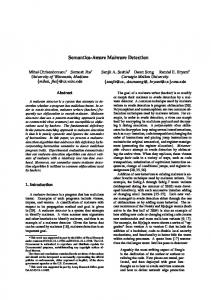
It is experimentally demonstrated in [10] that for metamorphic malware detection bi–gram feature outperforms uni– gram attributes. Present study showed high variability in frequency of bi–grams in malware and in benign model (refer Figure 2). Thus, bi–gram features generated from uni–gram are extracted from train and test set. From training set 6923 opcodes are obtained. Subsequently, 2769 features are selected based on their prominence in training file (refer Figure 1). B. Rank Feature Pruned bi–gram feature space is further ranked using feature selection methods (refer Figure 3) such as Term Frequency-Inverse Document Frequency (TF-IDF), Term Frequency-Inverse Document Frequency-Class Frequency (TF-IDF-CF), Categorical

Frequency Variation of Bi–gram Opcodes in Target Class

Proportional Distance (CPD), Galavotti-Sebastiani-Simi Coefficient (GSS), Weight of Evidence of Text (WET), Term Significance (TS), Odds Ratio (OR), Weighted Odds Ratio (WOR) Multi-Class Odds Ratio (MOR) Comprehensive Measurement Feature Selection (CMFS) and Accuracy2 (ACC2). Feature selection techniques can be broadly categorized as (a) feature search and (b) feature subset evaluation [33]. Feature can be picked using exhaustive, sequential or random searches that improves the classification. Whereas, in feature subset approach a collection of fewer feature is extracted from a larger feature space that enhances the accuracy. Usually, subset methods are segregated into filter and wrapper approaches [32]. Following are the advantages of attribute selection techniques. • Reduced feature length drastically alleviate classification time and memory requirements. • Provides better visualization and knowledge of dataset. • Remove redundant features resulting in maximum discriminant features that contribute towards classification. 1) Term Frequency-Inverse Document Frequency (TFIDF): TF-IDF score [15] of a bi–gram feature j for a sample i belonging to a class is computed as, ! N + 1.0 ai,j = log(tfi,j + 1.0) ∗ log (1) nj where, tfi,j : Frequency of opcode j in sample i. N : Total number of training samples. nj : Total occurrences of opcode j in training set. 2) Term Frequency-Inverse Document Frequency-Class Frequency (TF-IDF-CF): TF-IDF-CF [16] score for a bigram feature j in ith specimen is calculated as, ! N + 1.0 nc,i,j ai,j = log(tfi,j + 1.0) ∗ log ∗ (2) nj nc,i where, tfi,j : Frequency of bi–gram j in sample i.



Nt : Total malware and benign samples consisting of bi–gram feature t. 4) Galavotti-Sebastiani-Simi Coefficient (GSS): GSS Coefficient [18] for a bi–gram feature tk is obtained as, GSS(tk , Ci ) = P (tk , Ci ).P (tk , Ci ) − P (tk , Ci ).P (tk , Ci ) (4) where, P (tk , Ci ) : Joint probability of an opcode tk with respect to class Ci . P (tk , Ci ) : Joint probability of absence of an opcode tk in class Ci . P (tk , Ci ) : Joint probability of an opcode tk with respect to class Ci . P (tk , Ci ) : Joint probability of absence of opcode tk with respect to class Ci . Ci and Ci : Represent malware (M) and benign (B) class. 5) Weight of Evidence of Text (WET): Weight of evidence of text [15] for a feature f is obtained as, ! m X P (Ci |f ).(1 − P (Ci ) W ET (f ) = P (Ci ).P (f ).log P (Ci ).(1 − P (Ci |f ) i=1 (5) where, P (Ci ) : Prior probability of classes. P (f ) :Prior probability of bi–gram feature f . Fig. 3.

Feature Ranking and Classification

P (Ci |f ) : Conditional probability of class Ci given the probability of feature f .

N : Total number of training specimens.

m : Total number of classes

nj : Number of occurrences of opcode j in training documents.

6) Term Significance (TS): Term significance [19] score of a bi–gram feature t with respect to class C is determined as,  log(max{P (t),P (C)})   1−log(min{P (t),P (C)}) , if P (t, C) = 0 T S(t, C) = (6)   log(max{P (t),P (C)})−log(P (t,C))

nc,i,j : Number of files in which bi–gram j belonging to class c where file i is a member. nc,i : Total number of files in class c (malware/benign), where i is a member. 3) Categorical Proportional Distance (CPD): Categorical proportional distance [17] of a feature t in class Ck is defined as, Nt,Ck − Nt,Ck (3) CP D(t, Ck ) = Nt where, Nt,Ck : Number of samples in class Ck consisting of bi–gram feature t. Nt,Ck : Number of specimens in class Ck containing bi–gram feature t.

1−log(min{P (t),P (C)})

where, P (t) : Marginal probability of bi–gram t. P (C) : Prior probability of Class C.

P (t, C) : Joint probability of opcode t in class C. 7) Odds Ratio (OR): For a bi–gram feature f , Odds Ratio [20] with respect to class Ck is calculated as, ) ( P (f |Ck ).(1 − P (f |Ck )) (7) OR(f, Ck ) = log P (f |Ck ).(1 − P (f |Ck ))


IAENG International Journal of Computer Science, 42:2, IJCS_42_2_09 ______________________________________________________________________________________ where, P (f |Ck ) : Conditional probability of bi–gram f given the probability of class Ck . P (f |Ck ) : Conditional probability of bi–gram f given probability of class Ck . 8) Weighted Odds Ratio (WOR): Weighted Odds Ratio [21] score for a feature f is determined as W OR(f ) =

C X

P (C).OR(f, C)

(8)

k=1

where, P (C) : Prior probability of class C. OR(f, C) : Odds score of bi–gram feature f with reference to class C. 9) Multi-Class Odds Ratio (MOR): Multi-Class Odds Ratio [21] of a feature f is obtained as, ( ) X P (f |Cj ).(1 − P (f |Cj )) M OR(f ) = log (9) P (f |Cj ).(1 − P (f |Cj )) j where, P (f |Cj ) : Conditional probability of feature f given probability of Cj .

P (f |Cj ) : Conditional probability of bi–gram f for known probability of target class Cj . 10) Comprehensive Measurement Feature Selection (CMFS): Comprehensive Measurement Feature Selection [22] for a bi–gram tk in class Ci is evaluated as, CM F S(f, Ci ) = P (f |Ci ).P (Ci |f )

(10)

where, P (f |Ci ) : Conditional probability of feature f given probability of class Ci . P (Ci |f ) : Conditional probability of class Ci given probability of bi–gram feature f . 11) Accuracy2 (ACC2): Accuracy2 [23] of a feature f in class Ci is computed as, ACC2(f, Ci ) = P (f, Ci ) − P (f, Ci ) (11)

where, P (f, Ci ) : Joint probability of feature f in class Ci .

P (f, Ci ) : Joint probability of feature f in class Ci .

C. Model Generation and Prediction Bi–gram feature space is sorted in the decreasing order of their ranks obtained with feature selection methods. Besides WET, WOR, MOR and ACC2, feature selection methods such as TF-IDF, TF-IDF-CF, CPD, GSS, TS, OR and CMFS are

used to acquire discriminant features pertaining to target classes (malware and benign) as discussed in Algorithm 1. Relevant bi–gram with variable lengths are used for constructing malware/benign model. Further, learning models are prepared using classification algorithms such as J48, AdaboostM1(using J48 as base classifier) and Random forest implemented in WEKA [24] with default settings. Algorithm 1 Selecting Discriminant Bi–grams of a Class INPUT: (a) O = {b1 ,b2 ......,bN } // Bi–gram opcodes (b) C = {M,B} // Malware or Benign class (c) FS = m1 ,m2 .......,mp // Ranking methods B M B OUTPUT: (a) {DListM m1 ,DListm1 ,.....,DListmp,DListmp }. 1: 2: 3: 4: 5: 6: 7: 8: 9: 10: 11: 12: 13: 14: 15: 16: 17: 18: 19: 20:

for i ← 1to|F | do DListM ⊲ Initialize the discriminant list m1 ← 0 DListB m1 ← 0 end for for p ← 1to|O| do for q ← 1to|F S| do for r ← 1to|C| do ⊲ Computing relevancy score index[r] ← Score(bp , mq ) end for Cid ← M axScore(temp[1], temp[2], .., temp[|C|] ⊲ Return class index with maximum size Cid DListCid mq ← DListmq ∪ (bp , temp[Cid]) end for end for for p ← 1to|F S| do for q ← 1to|C| do Sort(DListqmp ) ⊲ Sort bi–gram opcodes in ⊲ decreasing order of their relevance end for end for

Motivated by a prior work in [25], prediction models obtained from tree based classifiers such as Adaboost and Random Forest are given stronger preference. Models are evaluated using metrics such as accuracy, precision, true positive rate and false positive rate by feeding unseen samples (not used in feature selection phase) to the previously constructed models. D. Comparison of Feature Selection Methods Models generated with feature selection methods perform differently on varying feature length. Therefore, to determine prominent feature selection method at a given feature length McNemar test [7] is employed. McNemar test is a nonparametric approach that follows chi–square distribution. Contingency table obtained for feature selection technique at a specific length is supplied as input for statistical testing. The method is based on acceptance or rejection of null or alternate hypothesis based on the computed chi–square value as in Equation 12. χ2 =

(|Q − R| − 1)2 Q+R

where, Q : Number of malwares misclassified as benign. R : Number of benigns misclassified as malware.


(12)

IAENG International Journal of Computer Science, 42:2, IJCS_42_2_09 ______________________________________________________________________________________ Computed chi–square value is further compared with tabulated value (i.e. is 3.84 in the present case). If the computed value is less than tabular value, null hypothesis is accepted else alternate hypothesis is considered.

•

•

•

Fig. 4.

Contingency Table

IV. E XPERIMENT

AND

F INDINGS

Experiments have been conducted on a computer system employing an Intel Core i3 processor with a RAM capacity of 4GB on a Linux 12.04 operating system. Extensive experimentation following investigations have been carried out: • • • •

Effect of feature length on classification accuracy. Feature selection methods that can produce better accuracy with optimal feature length. Bi–gram opcodes that are predominantly used for generating morphed malware copies. Suitable classifiers to be used for developing malware scanner.

A. Dataset Malware data set consisting of 868 samples of NGVCK viruses and metamorphic worm as in [26] have been considered in afore mentioned experiments. Prior studies in [26] reported that highly morphed NGVCK samples could easily bypass strong statistical detector based on HMM. Likewise, 1218 executables including games, web browsers, media players and executables of system 32 (Windows XP operating system) are considered as benign set. Before including the samples in benign set, they were scanned with commercial antivirus scanners to assure that none of the benign samples are infected. Entire data set is divided into two equal portions where training model is prepared from nearly 50% of samples and remaining files are reserved for prediction phase. B. Evaluation Parameters Performance for diverse feature length are evaluated using accuracy, precision, true positive and false positive rate. These evaluation parameters are determined from True Positive (TP), True Negative (TN), False Negative (FN) and False Positive (FP) rates (refer Figure 4). TP is the number of correctly identified malware samples, FN is the number of incorrectly classified malware specimens, TN the number of correctly identified benign samples and, FP is the number of benign files misclassified as malware. A brief introduction to the evaluation parameters have been presented as follows(refer Equations 13 through 16)

•

Accuracy (Acc) is the ratio of correctly classified instances in the dataset TP + TN Acc = (13) TP + FN + TN + FP Precision (P) is the ratio of number of files that are correctly classified as malware to the total number of correctly identified malware samples and benign files misclassified as malware. TP P = (14) TP + FP True Positive Rate (TPR) corresponds to the proportion of malware samples correctly predicted by the classification model. TP TPR = (15) TP + FN False Positive Rate (FPR) is the proportion of malware samples misclassified as benign. FPR =

FP TN + FP

(16)

C. Results Feature ranking methods such as TF-IDF, TF-IDF-CF, CPD, GSS Coefficient, WET, TS, OR, WOR, MOR, CMFS and ACC2 are applied to pruned 2769 bi–gram features. In this article the impact of classification accuracy at variable feature length is researched. A bi–gram feature is said to be discriminant to a class, if it is prominent in a specific class compared to other. It has been observed that for TF-IDF, TF-IDF-CF, GSS Coefficient, OR and CMFS model constructed with discriminant malware feature (10 features) furnished 100% accuracy (refer Figure 5 through 9). Likewise, MOR features displayed an accuracy of 100% at a reduced feature length of 10 (refer Figure 21). Further reduction of feature space below ten bi–grams drops the classification accuracy. This is because, features that contribute towards classification are eliminated from feature space. However, TF-IDF-CF and TF-IDF discriminant benign features also yielded 100% accuracy with feature length of 200 and 300 respectively. It is because benign bi–gram samples are diverse and large number of features are required for classification (refer Figure 12 and Figure 13). GSS discriminant benign features resulted in an accuracy of 99.8% at feature length of 40 and 100 respectively (refer Figure 14). Further increase in feature space does not improve accuracy and at 800 feature length 100% accuracy is obtained. We choose top 40 discriminant benign GSS features as optimal feature length because only 0.2% increase in accuracy is achieved by increasing feature space from 40 to 800. Adding extra 760 features increases processing overhead. For CPD feature selection, discriminant malware features resulted in 100% accuracy and precision at feature length of 200 bi–grams (refer Figure 10). Moreover CPD discriminant benign features resulted in 99.8% accuracy at 800 feature length (refer Figure 17). It is because CPD renders higher rank for features that fall only in a class even present in few samples. TS discriminant malware depicts an accuracy of 100% at a feature length of 800 (refer Figure 11), whereas TS



98

98

96

96

Accuracy

100

Accuracy

100

94

94

92

92

90

90 10

20

30

40

50

10

20

Feature Length AdaBoostM1

J48

Fig. 5.

30

40

50

Feature Length RandomForest

Evaluation Metrics for TF-IDF(Discriminant Malware Features)

AdaBoostM1

J48

Fig. 7.

RandomForest

Evaluation Metrics for GSS(Discriminant Malware Features)

100 100 98

96

Accuracy

Accuracy

98

96

94

94 92 92 90 90

10 10

20

30

40

AdaBoostM1

30

40

50

Feature Length

Feature Length J48

20

50

AdaBoostM1

J48

RandomForest

RandomForest

Fig. 8.

Evaluation Metrics for OR(Discriminant Malware Features)

Fig. 6. Evaluation Metrics for TF-IDF-CF(Discriminant Malware Features)

100

98

Accuracy

discriminant benign features results in an accuracy of 99.9%, 99.8% at 700 and 400 bi–grams (refer Figure 18). Thus, for TS discriminant benign features, optimal feature length is considered as 400 since there is only a marginal increase in accuracy if feature space is substantially increased. OR and WOR discriminant bi–grams resulted in 99.8% accuracy for 40 feature length (refer Figure 15 and Figure 20). Further increase in bi–gram feature space reduces accuracy and later remains constant. It is also observed that CMFS benign features depicts an 100% for 50 bi–gram features (refer Figure 16).

96

94

92

90

Moreover, WET and ACC2 ranked bi–gram feature resulted in 100% accuracy at 20 and 30 feature length. It is noticed that because of increased false alarms, accuracy drops when feature length is dropped below 10 (refer Figure 19, Figure 22).

10

20

J48

Fig. 22.

30 40 Feature Length AdaBoostM1

Evaluation Metrics for ACC2


50

100 RandomForest


98

98

96

96

Accuracy

100

Accuracy

100

94

92

94

92

90

90 10

20

30

40

50

100

50

100

200


J48

Fig. 9.

RandomForest

500

AdaBoostM1

J48

Fig. 11.

100

600

700

800

RandomForest

Evaluation Metrics for TS(Discriminant Malware Features)

100

98

98

96

Accuracy

Accuracy

400

Feature Length

Evaluation Metrics for CMFS(Discriminant Malware Features)

94

92

96

94

92

90 10

20

30

J48

Fig. 10.

300

40 50 100 Feature Length AdaBoostM1

200

90

300

50

RandomForest

J48

D. Comparative Analysis of Feature Selection Methods Here, feature selection methods are analysed (refer Table II). From experimental results, it can be argued that discriminant malware features extracted using feature ranking methods are prominent than benign features. TABLE II C OMPARATIVE A NALYSIS OF F EATURE S ELECTION M ETHOD BASED ON A CCURACY WITH D ISCRIMINANT M ALWARE F EATURES Feature Length

TF-IDF TF-IDF-CF GSS OR CMFS MOR WET ACC2 WOR CPD TS

10 10 10 10 10 10 20 30 40 200 800

200

300

400

500

Feature Length

Evaluation Metrics for CPD(Discriminant Malware Features)

Feature Selection

100

Accuracy with Random forest Classifier 100 100 100 100 100 100 100 100 99.80 100 100

Rank 1 1 1 1 1 1 2 3 4 5 6

It is observed that for increased feature space using TF-IDF, TF-IDF-CF, GSS, OR, CMFS and MOR feature

Fig. 12.

AdaBoostM1

RandomForest

Evaluation Metrics for TF-IDF(Discriminant Benign Features)

selection techniques with malware features, the accuracy remains constant beyond 10 prominent opcodes. However, in case of benign features larger number of attributes are used to develop the model. This is because benign samples are diverse and usually written in high level language. Hence, the common opcodes are rare due to diversification. Whereas, malware programs are author specific (written in low level language) or generated using metamorphic engine. Thus the appearances of common opcodes are more likely to be present in variants of base files. These opcodes are retained by metamorphic engine to preserve maliciousness. Also the complete transformation of x86 assembly code with equivalent sets of opcode is difficult to be implemented. Therefore, it is likely that a malware model may be generated but a generic benign model is difficult to be developed. Stronger preference for the model generated by Random Forest as well as Adaboost is given. This is because Random Forest [27] is an ensemble of many trees (also known as learners) where, each tree vote for a class. The classifier accumulates votes from entire trees in the forest to categorize new instance. Bagging and boosting properties enhances the


IAENG International Journal of Computer Science, 42:2, IJCS_42_2_09 ______________________________________________________________________________________ TABLE III T OP 10 DISCRIMINANT MALWARE BI – GRAM OPCODES WITH TF-IDF, TF-IDF-CF, GSS, OR, CMFS AND MOR TF-IDF jemov testje cmpje jnemov testjne movsxdmov movmovsxd cmpjne jmpnop jecmp

TF-IDF-CF jemov testje cmpje jnemov cmpjne testjne movsxdmov movmovsxd jmpnop jecmp

GSS jemov cmpjne cmpje retpush jeadd jecmp jnejmp testje jnemov testjne

OR jemov cmpjne cmpje retpush jeadd jecmp jnejmp testje jnemov testjne

CMFS jemov cmpjne cmpje retpush jeadd jecmp jnejmp testje jnemov testjne

MOR jemov cmpjne cmpje retpush jeadd jecmp jnejmp testje jnemov testjne

TABLE IV M EAN VALUES FOR P ROMINENT F EATURES opcode jemov testje cmpje jmpnop jnemov testjne cmpjne jecmp movmovsxd movsxdmov jnejmp jeadd retpush

TF-IDF M B 203.10 0 199.54 0 165.49 0 121.79 0.05 115.57 0 111.40 0 101.87 0 88.84 0 86.73 0.50 86.18 0.56 27.52 0 17.67 0 6.97 0

TF-IDF-CF M B 203.10 0 199.54 0 165.49 0 121.79 0.05 115.57 0 111.40 0 101.87 0 88.84 0 86.73 0.50 86.18 0.56 27.52 0 17.67 0 6.97 0

Feature Selection Method GSS OR M B M B 203.10 0 203.10 0 199.54 0 199.54 0 165.49 0 165.49 0 121.79 0.05 121.79 0.05 115.57 0 115.57 0 111.40 0 111.40 0 101.87 0 101.87 0 88.84 0 88.84 0 86.73 0.50 86.73 0.50 86.18 0.56 86.18 0.56 27.52 0 27.52 0 17.67 0 17.67 0 6.97 0 6.97 0

CMFS M B 203.10 0 199.54 0 165.49 0 121.79 0.05 115.57 0 111.40 0 101.87 0 88.84 0 86.73 0.50 86.18 0.56 27.52 0 17.67 0 6.97 0

MOR M B 203.10 0 199.54 0 165.49 0 121.79 0.05 115.57 0 111.40 0 101.87 0 88.84 0 86.73 0.50 86.18 0.56 27.52 0 17.67 0 6.97 0

TABLE V E XPERIMENTAL R ESULTS WITH R ANDOM F OREST USING T OP 10 S IGNIFICANT F EATURES Feature Selection Method TF-IDF TF-IDF-CF CPD GSS WET TS OR WOR MOR CMFS ACC2

TPR(%) 100 100 78.29 100 100 97.69 100 100 100 100 100

FPR(%) 0 0 0 0 2.95 17.40 0 2.95 0 0 3.11

performance of Random Forest classifier. Performance of decision tree classifiers (J48) is marginally less in comparison to Random Forest and Ababoost. In J48 the decision of splitting a node is performed by gathering information gain determined over all attributes. However, Random Forest picks few attributes in random that have higher probability in identifying a target class. This characteristic of the Random Forest classifier would facilitate in scaling up a model if original feature space is enormous. Moreover, the attributes selected by this classifier are less correlated. A perfect malware detector should have very high True Positive Rate (TPR) along with less False Positive Rate (FPR). Also, the time to predict test samples using different feature selection methods is closer to those of commercial antiviruses (refer Table V). V. I NFERENCE 1) What is the effect of feature length on classification accuracy? It is observed that small feature length has higher classification accuracy and a further increase

Accuracy 100 100 90.97 100 98.27 88.86 100 98.27 100 100 98.17

Time in Microseconds 0.000579 0.000593 0.000643 0.000594 0.000611 0.000748 0.000629 0.000642 0.000614 0.000584 0.000627

of features deteriorates the performance. If features discriminant to malware are used for model creation, higher accuracy is obtained at minimal feature space. Thus it characterizes that the dataset used in our study has large number of discriminant features pertaining to malware with less diversification. 2) Which classifier results in improved performance? Tree based classifiers like Adaboost and Random Forest resulted in higher preference because they use bagging and boosting approach for classification. Random forest classifier is given higher preference than any other classifiers as reported in prior studies [27]. 3) Which category of feature is better? Bi–gram features that are discriminant to malware class are used extensively for model preparation. Since malicious code is written in low level language, there exists certain bi– gram features intended to represent malignity which needs to be retained in successive generations. Benign files are written in diverse high level language, the features discriminant to benign samples are distinct and


100

100

98

98

96

96

Accuracy

Accuracy


94

92

94

92

90

90 10

20

30

40

50

10

20

30


J48

RandomForest

50

100

200

Fig. 15.

100

100

98

98

96

96

94

92

AdaBoostM1

J48

Accuracy

Accuracy

Fig. 13. Evaluation Metrics for TF-IDF-CF(Discriminant Benign Features)

300

RandomForest

Evaluation Metrics for OR(Discriminant Benign Features)

94

92

90

90 10

20 J48

Fig. 14.

40

Feature Length

30

40 50 100 Feature Length AdaBoostM1

200

300

10 J48

RandomForest

Evaluation Metrics for GSS(Discriminant Benign Features)

a universal representation of feature that is required to identify benign files cannot be represented. Thus these features are scarce even after attribute selection algorithm are utilized. Top ten malware bi–gram features for robust feature selection methods that results in 100% accuracy are shown in Table III. Table IV presents mean values of top ranked bi– gram opcodes obtained from feature selection methods. These features are arranged based on their contribution towards classification. We observe that there is a significant difference in mean values of bi–grams in both the target classes. As a result, these top ranked features could identify unseen samples with better accuracy. 4) Which feature selection method result in robust feature space? The appropriateness of feature selection methods (abbreviated as M i eg: M 1, M 2...M 11. M i − M and M i − B designate discriminant malware and benign features extracted using method M i) are evaluated using McNemar Test [7]. McNemar Test is applied to feature selection methods at distinct feature length by determining the Chi–Square value. If the computed

20

Fig. 16.

30 40 Feature Length AdaBoostM1

50

100 RandomForest

Evaluation Metrics for CMFS(Discriminant Benign Features)

Chi–Square value of a give feature selection approach is found to be less in comparison with the tabular value then such methods are considered significant. This indicate acceptance of null hypothesis, i.e. if computed value is less than 3.84 (standard value) otherwise alternate hypothesis is considered. Also, in certain cases optimality of feature selection methods for chi– square value less than 3.84 is discarded considering large feature space. Table VI depict the McNemar Test score for different feature selection methods for variable feature length obtained with a feature selection technique. Each cell in table represents calculated chi– square value. Likewise, Figure 23 shows the feature length and classification accuracy represented using different patterns. In this figure, the cells with diagonal pattern indicate 100% accuracy. It can be observed that for discriminant malware features TF–IDF, TF– IDF-CF, GS, OR and CMFS produces 100% accuracy with 10 bi–grams. However, with benign features better accuracy is achieved at feature length beginning at 100 opcodes (shown in cells with horizontal pattern). Zones


50

100

200

300

400

500

600

700

800

Feature Length J48

Fig. 18.

AdaBoostM1

RandomForest

Evaluation Metrics for TS(Discriminant Benign Features)

with poor accuracy is indicated with black and light grey color. Also, models constructed with IG, WET, MOR and ACC2 perform well with fewer bi–grams. Thus, from this figure it can be concluded that the models created by pruning features using TF-IDF, TFIDF-CF, GS, OR, CMGS, IG, WET, MOR and ACC2 accurately identify unseen instances. VI. C ONCLUSIONS The research carried out here in the domain of metamorphic malware detection to develop a non–signature based scanner using feature ranking methods has been highly successful. Feature selection methods such as TF-IDF, TFIDF-CF, GSS, OR, CMFS and MOR resulted in the detection of MWORM and NGVCK viruses with 100% accuracy using top ten discriminant malware bi–grams. The significance of the feature selection methods using McNemar Test has been experimentally justified. Through the extensive experiments it can be argued that degree of metamorphism exhibited by MWORM and NGVCK is weak. Dead code added to the viruses can defeat any technique based on sequence

Significant Feature Selection Method ACC2 (M11)

16.05 2.25 1.33 0.50 1.33 1.33 0.50 1.33 0.50 1.33

0 0 0 0 0 0 0 0 0 0

CMFS (M10) M10-M M10-B 0 17.05 0 2.25 0 1.33 0 0.50 0 0 0 0.50 0 0 0 0 0 0 0 0 16.05 0 0 0 0 0 0 0 0 0

90

10 20 30 40 50 100 200 300 400 500

92

MOR (M9)

94

WOR (M8)

96

OR (M7) M7-M M7-B 0 16.05 0 2.25 0 1.33 0 0.50 0 1.33 0 1.33 0 0.50 0 1.33 0 0.50 0 1.33

Accuracy

98

TS (M6) M6-M M6-B 46.17 22.04 35.55 0 28.86 0 2.70 0 0.10 0.50 0.12 0

100

GSS (M5) M5-M M5-B 0 16.05 0 2.25 0 1.33 0 0.50 0 1.33 0 0.50 0 1.33 0 2.25 0 1.33 0 0.50

Evaluation Metrics for CPD(Discriminant Benign Features)

TF-IDF-CF (M4) M4-M M4-B 0 0 0 0 0 2.25 0 0 0 0 0 0 0 0 0 0

Fig. 17.

RandomForest

(M3) M3-B 2.25 1.33 0.50 0 0 0


J48

TF-IDF M3-M 0 0 0 0 0 0 0 0 0 0

100 200 300 400 500 600 700 800 900

(M2) M2-B 117.37 113.38 44.84 44.84 44.84 44.46

50

CPD M2-M 92.01 20.04 20.04 20.04 6.12 0 0 0 0 0

80

WET (M1)

85

Feature Length

90

TABLE VI M C N EMAR T EST S CORE FOR F EATURE S ELECTION M ETHODS AT DIFFERENT F EATURE L ENGTH ( CELLS SHADED DEPICT LOW ACCURACY I . E . HIGH C HI –S QUARE VALUE )

Accuracy

95

17.05 2.25 0 0 0 0 0 0 0 0

100

M3-M, M4-M, M5-M, M7-M, M9, M10-M M1, M3-M, M4-M, M5-M, M7-M, M9, M10-M M1, M3-M, M4-M, M5-M, M7-M, M9, M10-M, M11 M1, M3-M, M4-M, M5-M, M7-M, M9, M10-M, M11 M1, M3-M, M4-M, M5-M, M7-M, M9, M10-M, M10-B, M11 M1, M2-M, M3-M, M4-M, M4-B, M5-M, M6-B, M7-M, M9, M10-M, M11 M1, M2-M, M3-M, M4-M, M4-B, M5-M, M6-B, M7-M, M9, M10-M, M10-B, M11 M1, M2-M, M3-M, M3-B, M4-M, M4-B, M5-M, M6-B, M7-M, M9, M10-M, M10-B, M11 M1, M2-M, M3-M, M3-B, M4-M, M4-B, M5-M, M7-M, M9, M10-M, M10-B, M11 M1, M2-M, M3-M, M3-B, M4-M, M4-B, M5-M, M6-B, M7-M, M9, M10-M, M10-B, M11




McNemar Test at Varying Feature Length

100

100

98

98

96

96

Accuracy

Accuracy

Fig. 23.

94

92

94

92

90

90 10

20

30

40

50

100

10

20

30

Feature Length J48

Fig. 19.

AdaBoostM1

40

50

100

200

300

Feature Length RandomForest

Evaluation Metrics for WET

Fig. 20.

alignment, but approach similar to one presented here can capture such opcodes as they are effectively synthesized during feature selection phase. Thus, the statistical scanner developed can be used for detecting complex metamorphic malware. In future, experiments are likely to be extended on a larger dataset and real metamorphic samples in wild. Moreover, other robust feature selection methods along with their combinations will also be explored. ACKNOWLEDGMENT We would like to thank Professor Mark Stamp of SJSU California for sharing the metamorphic malware dataset for conducting this study.

AdaBoostM1

J48

RandomForest

Evaluation Metrics for WOR

R EFERENCES [1] M. Stamp. Information Security: Principles and Practice. John Wiley & Sons, 2011. [2] Wong, Wing and Stamp, Mark, Low Richard M and Stamp Mark. Hunting for metamorphic engines. Journal in Computer Virology, Vol. 2: 211-229, 2006. [3] S. Attaluri, S. McGhee, and Stamp Mark. Profile hidden Markov models and metamorphic virus detection. Journal in Computer Virology, Vol. 5, No. 2, pp. 151-169, 2009. [4] Madenur Sridhara, Sudarshan and Stamp Mark. Metamorphic worm that carries its own morphing engine. Journal of Computer Virology and Hacking Techniques, vol.(9), pp. 49-58, 2013. [5] Annie H T, Mark S. Chi-squared distance and metamorphic virus detection. In Journal in Computer Virology Vol. 9 No. 1 pp. 1-14, 2013. [6] Baysa Donabelle , Low Richard M and Stamp Mark. Structural entropy and metamorphic malware. Journal of Computer Virology and Hacking Techniques, Springer-Verlag, pp. 1-14, 2013. [7] Robert G. Lehr. Encyclopedia of Biopharmaceutical Statistics, Third Edition, ISBN 9781439822456, May 2010. [8] N. Runwal, R. M. Low and Mark Stamp. Opcode graph similarity


IAENG International Journal of Computer Science, 42:2, IJCS_42_2_09 ______________________________________________________________________________________ 100

Accuracy

98

96

94

92

90 10

20

30

40

50

Feature Length J48

Fig. 21.

AdaBoostM1

RandomForest

Evaluation Metrics for MOR

and metamorphic detection. Journal in Computer Virology, 8(1-2):3752, 2012. [9] M.E. Saleh, A.B. Mohamed, A. Nabi. Eigenviruses for metamorphic virus recognition. In IET Information Security (Inf. Secur), Vol.5, Iss. 4, pp. 191-198, 2011. [10] Vinod P, Vijay Laxmi, Manoj Singh Gaur,G.V.S.S Phani Kumar and Yadvendra S Chundawat. Static CFG analyzer for metamorphic Malware code. In Proceedings of the 2nd International Conference on Security of Information and Networks, SIN 2009, Gazimagusa, North Cyprus, October 6-10, pp: 225-228, 2009. [11] Vinod P, Harshit Jain, Yashwant K Golecha, Manoj Singh Gaur and Vijay Laxmi. MEDUSA:MEtamorphic malware dynamic analysis using signature from API. In Proceedings of the 3rd International Conference on Security of Information and Networks, SIN 2010, Rostov-on-Don, Russian Federation, September 7-11, pp: 263-269, 2010. [12] Vinod P, Laxmi V, Gaur M S, Chauhan G. MOMENTUM: MetamOrphic malware Exploration Techniques Using MSA signatures. Innovations in Information Technology(IIT), 2012 International Conference, pp.232-237, 2012. [13] Sushant Priyadarshi and Mark Stamp. Metamorphic detection via emulation. Masters report, Department of Computer Science, San Jose State University, 2011. [14] Jikku Kuriakose, Vinod P. Ranked linear discriminant analysis features for metamorphic malware detection. In Proceedings of 4th IEEE International Advanced Computing Conference (IACC-2014), Gurgaon, India, pp.112 - 117, 21-22 February-2014. [15] Shang, Wenqian and Huang, Houkuan and Zhu, Haibin and Lin, Yongmin and Qu, Youli and Wang, Zhihai. A Novel Feature Selection Algorithm for Text Categorization. In Journal of Expert Syst. Appl., vol.(33), number(1), pp 1-5, July, 2007. [16] Mingyoug Liu and Jiangang Yang. An improvement of TFIDF weighting in text categorization. International Conference on Computer Technology and Science (ICCTS 2012), Singapore, IPCSIT vol.47,2012. [17] Mondelle Simeon, and Robert J. Hilderman. Categorical proportional distance: A feature selection method for text categorization. AusDM, volume 87 of CRPIT, page 201-208. Australian Computer Society, 2008. [18] Zheng Z and Srihari R. Optimally combining positive and negative features for text categorization. In workshop for learning from imbalanced datasets, Proceedings of ICML, 2003. [19] Basu T and Murthy, C.A. Effective Text Classification by a Supervised Feature Selection Approach. In Proceedings of 12th IEEE International Conference on Data Mining Workshops(ICDMW), Los Alamitos, CA, USA, pp 918 - 925, December, 2012. [20] Zhaohui Zheng, Xiaoyun Wu, and Rohini K. Srihari. Feature selection for text categorization on imbalanced data. SIGKDD Explorations 6(1):80-89 ,2004. [21] Al-Rousan, Nabil M, Haeri, Soroush and Trajkovic Ljiljana. Feature selection for classification of BGP anomalies using Bayesian models. In proceedings of ICMLC, IEEE, pp. 140-147, 2012. [22] Yang Jieming, Liu Yuanning, Zhu Xiaodong, Liu Zhen and Zhang Xiaoxu. A new feature selection based on comprehensive measurement both in inter-category and intra-category for text categorization. Inf. Process. Manage. Volume=48:741-754, 2012.

[23] Forman G.. An Extensive Empirical Study of Feature Selection Metrics for Text Classification. Journal of Machine Learning Research 3, pp. 12891305, 2003. [24] M. Hall, E. Frank, G. Holmes, B. Pfahringer, P. Reutemann, Ian H. Witten. The WEKA Data Mining Software: An Update. SIGKDD Explorations, Volume 11, Issue 1,2009. [25] Vinod P, Vijay, L, Manoj, S.G., Smita, N., Parvez, F. MCF: MultiComponent Features for Malware analysis. In Proc of 27th IEEE International Conference on Advanced Information Networking and Applications (AINA-2013), Barcelona, Spain, March 25-28, 2013. [26] D. Lin, M. Stamp, Hunting for undetectable metamorphic viruses. Journal in Computer Virology, Vol. 7, No. 3, pp. 201-214, 2011. [27] Breiman, L, Random forest. Machine Learning. 45 (1):532 doi: 10.1023/A: 1010933404324, 2001. [28] J. Zico Kolter and Marcus A. Maloof, Learning to detect and classify malicious executables in the wild, Journal of Machine Learning Research, 2006, vol.7, pp.2741–2745. [29] Tahan, G.; Rokach, L. and Shahar, Y. (2012), ’Mal-ID: Automatic Malware Detection Using Common Segment Analysis and Meta-Features.’, Journal of Machine Learning Research, 2013 , pp.949-979 . [30] Zongqu Zhao; Junfeng Wang; Jinrong Bai, “Malware detection method based on the control-flow construct feature of software”, Information Security, IET , vol.8, no.1, pp.18,24, Jan. 2014. [31] O’Kane, P.; Sezer, S.; McLaughlin, K.; Eul Gyu Im, “SVM Training Phase Reduction Using Dataset Feature Filtering for Malware Detection”, Information Forensics and Security, IEEE Transactions on, vol.8, no.3, pp.500,509, March 2013. [32] Kumar, R. Kishore, G. Poonkuzhali, and P. Sudhakar, “Comparative study on email spam classifier using data mining techniques”, Proceedings of the International MultiConference of Engineers and Computer Scientists. Vol. 1. 2012. [33] Lin, Pengpeng, et al. “Feature Selection: A Preprocess for Data Perturbation”, IAENG International Journal of Computer Science 38.2 (2011): 168-175.

Jikku Kuriakose : Completed his Master in Technology in Computer Science and Engineering with specialization in Information Systems from SCMS School of Engineering and Technology, Cochin, Kerala, India. He earned B.E. in Computer Science and Engineering from Anna University, Chennai, India. His area of interest include metamorphic malware analysis and detection techniques, software reverse engineering and data mining. He has published articles in the domain of malware analysis in reputed book chapters and international conferences. Vinod P: Vinod P. is an Associate professor in Department of Computer Science and Engineering at SCMS School of Engineering and Technology, Kerala, India. He received his PhD in Malware Analysis and Detection methodologies from Malaviya National Institute of Technology, Jaipur, India. His current area of interest is Desktop and Android malware detection methods, intrusion detection, ethical hacking, algorithms and sentiment analysis. He has widely published 55 papers in reputed international conferences, book chapters and journals. He is also a member of technical program committees in the domain of information and network security.
