Bars, Per Berglund, Peter Bouwknegt, Andreas Brandhuber, Michael Douglas, Pedro. Fonseca, Jaume Gomis, Christiaan Hofman, Sameer Murthy, Dennis ...
RUNHETC-2002-48 USC-02/08 hep-th/0211291
Unoriented Strings, Loop Equations, and N = 1
arXiv:hep-th/0211291v3 16 Dec 2002
Superpotentials from Matrix Models
Sujay K. Ashok♭ , Richard Corrado♮ , Nick Halmagyi♮ , Kristian D. Kennaway♮ , and Christian R¨omelsberger♮ ♭
Department of Physics and Astronomy Rutgers University Piscataway, NJ 08540, USA
♮
Department of Physics and Astronomy University of Southern California Los Angeles, CA 90089, USA Abstract
We apply the proposal of Dijkgraaf and Vafa to analyze N = 1 gauge theory with
SO(N) and Sp(N) gauge groups with arbitrary tree-level superpotentials using matrix model techniques. We derive the planar and leading non-planar contributions to the large M SO(M) and Sp(M) matrix model free energy by applying the technology of higher-genus loop equations and by straightforward diagrammatics. The loop equations suggest that the RP2 free energy is given as a derivative of the sphere contribution, a relation which we verify diagrammatically. With a refinement of the proposal of Dijkgraaf and Vafa for the effective superpotential, we find agreement with field theory expectations. November 2002
Contents 1 Introduction
3
2 Results from N = 1 Gauge Theories
5
2.1 N = 2 Softly Broken to N = 1
. . . . . . . . . . . . . . . . . . . . . .
5
2.2 The N = 1∗ Theories . . . . . . . . . . . . . . . . . . . . . . . . . . . .
7
3 Calabi-Yau Geometry
9
4 The Classical Loop Equation
12
5 gs Corrections and Loop Equations
15
5.1 The Resolvent . . . . . . . . . . . . . . . . . . . . . . . . . . . . . . . .
16
5.2 The Loop Equation . . . . . . . . . . . . . . . . . . . . . . . . . . . . .
18
5.3 Solution to the Loop Equations . . . . . . . . . . . . . . . . . . . . . .
19
5.3.1 5.3.2
Planar Contributions . . . . . . . . . . . . . . . . . . . . . . . . 2
RP Contributions . . . . . . . . . . . . . . . . . . . . . . . . . 2
2
5.4 Counting Feynman diagrams with S and RP topology . . . . . . . . . 6 Computation of Effective Superpotentials
20 21 22 23
6.1 Non-Perturbative Sector . . . . . . . . . . . . . . . . . . . . . . . . . .
23
6.2 The N = 1∗ Theories . . . . . . . . . . . . . . . . . . . . . . . . . . . .
26
7 Discussion
26
A Matrix Integral Measures and Determinants
28
A.1 The Group Measure for General Matrices . . . . . . . . . . . . . . . . .
28
A.2 The Induced Measure of the N = 1∗ Theory . . . . . . . . . . . . . . .
29
B Asymptotic expansion of the gauge group volumes
30
C Matrix model Feynman rules and enumeration of diagrams
31
2
1
Introduction
Recently Dijkgraaf and Vafa [1, 2, 3] have proposed that the exact low-energy superpotential of certain N = 1 supersymmetric gauge theories is captured by the large M
behavior of certain associated M × M matrix models. This is quite remarkable, as
it reduces the problem of what is, in general, strongly-coupled physics of the confining phase of pure gauge theory to the zero-dimensional dynamics of a matrix integral.
Furthermore, the gauge theory quantities are computed from just the planar graphs of the matrix theory, nevertheless capturing finite N results in SU(N) gauge theory. The conjecture was initially tested for N = 2 SU(N) gauge theories softly broken
to N = 1 by a tree-level superpotential for the adjoint chiral superfields [1] and for the
N = 1∗ deformation of N = 4 SU(N) SYM [3, 4, 5]. The conjecture has since been
extended to a number of other cases [2, 6, 7, 8, 9, 10, 11, 12, 13, 14, 15, 16, 17, 18, 19, 20, 21, 22, 23, 24, 25, 26] and has been derived from SU(N) gauge theory [27, 28, 29]. In this work we use matrix techniques to analyze N = 1 gauge theory with SO(N)
and Sp(N) gauge groups. By a careful consideration of the planar and leading nonplanar corrections to the large M SO(M) and Sp(M) matrix models, we derive the matrix model free energy. We do this both by applying the technology of higher-genus loop equations of [30, 31] and by straightforward diagrammatics (see e.g. [32, 33]). The outline of the paper is as follows. In section 2, we discuss general features
of the four-dimensional gauge theories with N = 2 supersymmetry softly broken to N = 1. We also suggest a result for the superpotential of the N = 1∗ theory with
gauge group SO(2N) which is based on a generalization of a derivation of Dorey [34] for SU(N) gauge group. In section 3, we discuss the geometric engineering of the softly broken N = 2 gauge theories by wrapping D5-branes and O5-planes on compact cycles of generalized conifolds.
The corresponding matrix models are introduced and solved in the large M limit in section 4. As for SU(M), we find that the loop equation for the resolvent of the matrix model describes a Riemann surface which is identified with a factorization of the spectral curve of the N = 2 gauge theory. The large M solution of the matrix
models computes the special geometry of Type IIB string theory on the associated Calabi-Yau manifold.
In section 5, we discuss the application of the higher-genus loop equations to the computation of the RP2 contribution to the free energy. The loop equations take the
3
form of integral equations which give recursion relations between the contributions to the resolvent at each genus. They suggest a very simple solution for the RP2 contribution in terms of the sphere contribution. In fact, the one crosscap contribution to the resolvent ω1 satisfies
∂ω0 , (1.1) ∂S0 where ω0 is the contribution to the resolvent from the sphere. We verify this relationship ω1 = ±q
by explicitly enumerating several types of diagrams. We find that the contribution to the free energy F1 from RP2 and F0 from S 2 are related by F1 = ±q
∂F0 , ∂S0
(1.2)
where S0 is half of the ’t Hooft coupling for the SO/Sp component of the matrix group. We determine the proportionality constant q from the diagrammatics to be q =
gs . 4
Our results suggest a refinement of the proposal of Dijkgraaf and Vafa for the effective superpotential in the case of SO and Sp gauge groups. We find that Weff = QD5
∂F0 + QO5 G0 − 2πi τ S, ∂S
(1.3)
where QD5 is the total charge of D5-branes, QO5 is the total charge of O5-planes, F0
is the contribution to the matrix model free energy from diagrams with the topology of a sphere and G0 is proportional to F1 , the contribution to the free energy from RP2
diagrams. We use (1.3) to obtain results consistent with gauge theory expectations. In particular, the matrix model is consistent with the requirement that there is a degeneracy of the massive vacua of the gauge theory given by h, the dual Coxeter
number of the gauge group. In the case of the N = 1∗ SO(2N) theory, which we
discuss in section 6.2, we find that the critical value of the superpotential exactly
matches the result obtained from our gauge theory arguments in section 2. We end with a discussion of our results and point out several areas for future development. Various supporting technical calculations are contained in appendices. In the course of this work, two papers on matrix models with SO/Sp groups have appeared. In [10], aspects of the geometric engineering of the gauge theories, as well the leading order in M computation of the free energy of quartic orthogonal and symplectic matrix ensembles are discussed. We use a different basis of matrices and we account for the appearance of diagrams involving pairs of twisted propagators that are not including in the oriented theory. More recently, while this manuscript was in a final 4
stage, [35] appeared. These authors discuss a perturbative derivation of the matrix model along the lines of [28], including a discussion of RP2 corrections. Their results confirm aspects of the refinement (1.3) that we found was necessary for the computation of the gauge theory effective superpotential.
Results from N = 1 Gauge Theories
2
In this section we review some results about N = 2 and N = 1 supersymmetric gauge
theories, specifically the spectral curves and how they factorize when N = 2 is softly
broken to N = 1. We focus on the case of SO and Sp gauge groups (SU was treated in [36], which this discussion follows). 2.1
N = 2 Softly Broken to N = 1
As is well known [37, 38]1, the moduli space of N = 2 gauge theories is governed by a “spectral curve”, the periods of which give the masses of BPS objects in the theory
(W-bosons, monopoles and dyons). In [41, 42, 43] these spectral curves were found for the SO/Sp gauge groups. For a rank-r gauge theory, the spectral curve is a genus r hyperelliptic curve, y 2 = P2r+2 (x, {φi }),
(2.1)
where P2r+2 is a polynomial of degree 2r + 2 in the x that also depends on the moduli φi . The SO and Sp spectral curves can also be written as a genus 2r − 1 curve, y 2 = P2r (x2 , {φi}),
(2.2)
which is therefore symmetric under the Z2 action x 7→ −x and is a double cover of the genus N curve (2.1) via this map.
In N = 1 language, the N = 2 vector multiplet of the Yang-Mills theory is decom-
posed into an adjoint chiral superfield Φ and an N = 1 vector superfield V . N = 2
supersymmetry can be broken to N = 1 by an appropriate gauge-invariant superpo-
tential term for Φ. Because the trace of odd powers of matrices in the Lie algebra of SO(N)/Sp(N) vanishes, in contrast to the U(N) case discussed in [1,2,3], the superpotential deformation for SO(N)/Sp(N) only includes polynomial terms of even degree: 1
See [39, 40] for reviews.
5
Wtree (Φ) =
n+1 X gk Tr(Φ2k ). 2k k=1
(2.3)
A superpotential Wtree of order 2n + 2 breaks the gauge symmetry down to a direct product of n + 1 subgroups, e.g.: SO(N) → SO(N0 ) × U(N1 ) × . . . × U(Nn ),
(2.4)
where N = N0 + 2N1 + · · · + 2Nn .
The U(1) factors in this theory decouple in the IR. In the supersymmetric vacua
of the N = 1 theory r − n mutually local monopoles simultaneously become massless
and condense, leading to confinement of the gauge theory [36]. The condition that r − n mutually local monopoles become massless leads to a “factorization locus” in the
moduli space of the spectral curve, where r − n of the (non-intersecting) cycles of the spectral curve are simultaneously pinching off to zero-volume.
Imposing this condition is therefore equivalent to the factorization [44] 2
y =
r−n Y i=1
2
(x −
p2i )2
2n Y j=1
(x2 − qi2 ),
(2.5)
where pi 6= pj , qi 6= qj for i 6= j. On this locus we then obtain the “reduced spectral
curve”
2n Y y = (x2 − qi2 ), 2
(2.6)
j=1
which is a genus 2n − 1 curve. This curve parameterizes the N = 2 vacua that are not
lifted by the deformation to N = 1 (2.3). Notice that the factorized curves now have a similar form for SO and Sp, and the curve is still invariant under x 7→ −x (this implies
that the branch points come in pairs: (−qi , qi )). This reduced spectral curve will be derived from string theory in the following section by taking an orientifold action on the configuration of D-branes on a generalized conifold that engineers this N = 1 gauge theory.
The low-energy effective superpotential of these gauge theory can be obtained from the reduced spectral curve as discussed by [36, 44]. It will take the form � X� Weff = Nˆi Πi − 2πiτi Si , i
6
(2.7)
where 2πiSi are the periods of the meromorphic 1-form y dx around the A-cycles of the spectral curve, Πi the corresponding periods around the B-cycles, and Nˆi is SU(Ni ), Ni Ni (2.8) Nˆi = − 1 SO(Ni), 2 Ni + 1 Sp(Ni ). ˆi emerges in the matrix model by By contrast, we will find that the shift Ni 7→ N
considering the first subleading corrections to the large M expansion, coming from Feynman diagrams of topology RP2 . Recently the gaugino effective superpotential has been perturbatively derived from SU(N) gauge theory [27, 28, 29]. It is interesting to note that similar arguments2 to those of [28] can be used to argue that only diagrams with at most one boundary (if quark flavors are present) or crosscap will contribute to the gauge theory superpotential [3, 13, 16]. 2.2
The N = 1∗ Theories
The N = 1∗ theories arise as deformations of N = 4 Yang-Mills theory by mass terms for the three adjoint N = 1 chiral fields. The total superpotential is ! 3 X W = tr Φ1 [Φ2 , Φ3 ] + mi Φ2i
(2.9)
i=1
and the F-flatness conditions can be written as
[Φi , Φj ] ∝ iǫijk Φk .
(2.10)
Supersymmetric vacua are then obtained by embedding SU(2) representations into the gauge group G. In particular, for G = SU(N), the embeddings are classified by the P divisors d of N, leading to d|N d massive vacua [46].
Dorey [34] (see also [47]), following the approach of [48], compactified the theory
with SU(N) gauge group on a circle of radius R. The degrees of freedom of the effective 2 + 1–dimensional theory are r = rank(G) complex Abelian scalar fields Xa which are composed of the Wilson lines and the scalars dual to the massless photons of the theory. The moduli space of the theory is
2
M = Eτr /WG ,
(2.11)
We thank Jaume Gomis and Jongwon Park for discussions on this issue. The same observation about crosscap contributions was made in [35] and more recently for boundaries in [45].
7
where Eτ is the elliptic curve parameterized by each Xa and WG is the Weyl group of G.
By several arguments, including the relationship between the elliptic CalogeroMoser systems and the N = 2 theories which can be softly broken to the N = 1∗
theory, Dorey found that the superpotential of the 2 + 1–dimensional theory took the form W =c
X a>b
℘(Xa − Xb ),
(2.12)
where ℘(z) is the Weierstrass function. Dorey argued that the coefficient c was independent of the radius R, so that critical values of (2.12) (which depend on the modular parameter τ and not the Xa ) could be evaluated in the vacua of the theory and extrapolated directly to the R → ∞ limit.
It is interesting to ask what the generalization3 of (2.12) is to arbitrary gauge
groups G. The modular properties of the superpotential that were crucial to Dorey’s argument must still be preserved, so the superpotential should remain a sum of Weierstrass functions. An obvious guess for the argument of these functions is to replace P Xa − Xb by the sum over the positive roots α>0 α · X. The integrable systems ap-
proach [50, 51, 46, 52] to N = 2 theories is a promising route to this result. In fact,
D’Hoker and Phong [53, 54, 55] have determined the integrable systems that govern a large class of N = 2 theories with gauge group G. An application of the techniques
of [46, 34] to the soft breaking of these theories to N = 1∗ suggests that the correct superpotential for gauge group G is X X ℘(αL · X) + ℘ν(αS ) (αS · X) . W = c {αL >0}
(2.13)
{αS >0}
where αL,S are the long and short positive roots of the Lie algebra of G, respectively, and ℘ν (z) are the twisted Weierstrass functions ν−1 � X σ� ℘ν (z) = ℘ z + 2ωa . ν σ=0
(2.14)
defined in [53]. For non-simply laced groups, roots of only two different lengths appear: ν(α) = 1 for all long roots, ν(α) = 2 for all short roots of bn , cn f4 , while ν(α) = 3 for the short roots of g2 . 3
After an initial version of this paper appeared, we became aware of earlier work by Kumar and
Troost [49], where they also suggest the formula (2.13) and give many more arguments for its validity. We thank P. Kumar for making us aware of this.
8
For SO(2N), since it is simply-laced, twisted Weierstrass functions do not appear, and we obtain W =c
X a>b
[℘(Xa − Xb ) + ℘(Xa + Xb )] .
(2.15)
Following [34], we can evaluate this in the k th confining vacuum to find (up to an additive constant)
� W ∼ E2 (τ + k)/(2N − 2) ,
(2.16)
where E2 (τ ) is the second regularized Eisenstein series. It is tempting to conjecture that the result for arbitrary G will take this form with the obvious substitution of h, the dual Coxeter number of G for 2N − 2, but this remains to be verified.
3
Calabi-Yau Geometry
We now review the string theoretic engineering of a softly broken N = 2 gauge theory with SO/Sp gauge group [44,36,56,1]. We consider type IIB string theory compactified on the non-compact A1 fibration u2 + v 2 + w 2 + W ′ (x)2 = 0,
(3.1)
where W (x) is a degree n + 1 polynomial, which will later be related to the tree level superpotential. This fibration has singularities at the critical points of W (x). In the neighborhood of those singularities, we can introduce the coordinate x′ = W ′ (x). Then it is easy to see that the singularities are all conifold singularities. This generalized conifold can be de-singularized in two ways: it can be resolved or it can be deformed. The resolution is given by the surface ! ! λ1 u + iv w + iW ′ (x) −w + iW ′ (x)
u − iv
λ2
=0
(3.2)
in C4 × P1 . In this geometry each singular point is replaced by a P1 . These P1 ’s are disjoint, holomorphic, have the same volume and are homologically equivalent.
The latter property can be seen by making use of the fibration structure away from W ′ (x) = 0. This A1 fibration over the x plane induces a fibration of non-holomorphic S 2 ’s over the x plane. This S 2 cannot shrink to zero size as one approaches a critical point of W in the x plane, but it becomes the holomorphic P1 of the resolution. We can now construct a softly broken N = 2 U(N) gauge theory with tree level
superpotential W (x) by wrapping N D5-branes around the S 2 . This is an UV definition 9
of the theory. A classical supersymmetric vacuum is obtained by minimizing the volume of the D5-branes. This amounts to distributing a collection of Ni D5-branes over the n minimal-volume holomorphic P1 ’s at the critical points of W . The U(N) gauge symmetry is then spontaneously broken to U(N1 ) × · · · × U(Nn−1 ).
We now want to consider an orientifold of this theory4 . Since we started with a type
IIB theory on a Calabi Yau, we have to combine the worldsheet orientation reversal with a holomorphic involution of the Calabi-Yau (an anti-holomorphic involution would be appropriate for the IIA theory). Furthermore we want to fix one of the P1 ’s and act freely on the rest of the Calabi Yau geometry. This can be done if W (x) is an even polynomial of order 2n. In terms of the fibration structure of the Calabi-Yau this means that the critical points of W ′ (x) come in pairs (−xi , xi ) and one critical point is fixed at x0 = 0. Then (u, v, w, x, λ1, λ2 ) 7→ (−u, −v, −w, −x, λ1 , λ2 )
(3.3)
is a holomorphic involution of the geometry (3.2), which leaves only the P1 at u = v = w = x = 0 fixed. In the string theory this means that there is an O5-plane wrapping this P1 in the Calabi-Yau geometry. There are essentially two choices of O5-plane with which we can wrap the fixed P1 . They are distinguished by a different choice of worldsheet action and carry RR 5-form charge of ±1 (the RR charge of an Op± -plane is ±2p−5 in conventions where we count
the charge of N/2 D-branes but not their N/2 images). The orientifold contribution to the RR charge of objects wrapping the P1 will cause a shift in the coefficient N0 in the flux-generated superpotential on the deformed Calabi-Yau geometry, as explained below. Now we can construct a softly broken N = 2 SO(N)/Sp(N/2) gauge theory with
tree level superpotential W (x) by wrapping N D5-branes around the S 2 and then
performing the orientifold. The gauge symmetry is again broken SO(N) 7→ SO(N0) ×
U(N1 ) × · · · × U(Nn−1 ) or Sp(N/2) 7→ Sp(N0 /2) × U(N1 ) × · · · × U(Nn−1 ) respectively
with N = N0 + 2N1 + · · · + 2Nn−1 .
If we flow this ultraviolet theory to the infrared, there will be a confinement transi-
tion. In string theory this is described by a geometric transition in which the resolved conifold geometry with wrapped D5-branes and O5-planes is replaced by a deformed 4
Orientifolds were discussed in the A-model in [57, 56, 58, 59], while the discussion of [60] is more closely related to the B-model which is our interest here.
10
conifold geometry [61] u2 + v 2 + w 2 + W ′ (x)2 − f (x) = 0,
(3.4)
where f (x) is an even polynomial of degree 2n − 2. Such a polynomial represents
the most general normalizable deformation of the singular conifold that still respects the holomorphic involution (3.3). For a reasonably small f (x), each critical point of W ′ (x) is replaced by two simple zeros of W ′ (x)2 − f (x). This means that each P1i is
replaced by a 3-sphere Ai with 3-form RR-flux H through it, equal to the amount of
D5-brane and O5-plane charge on the P1i . The orientifold acts on one 3-sphere A0 as the antipodal map, while the other 3-spheres are mapped to each other in pairs Ai and A−i . Note that there is no orientifold fixed plane anymore.
The coefficients in f (x) are normalizable modes that are localized close to the tip
of the conifold. The coefficients in f (x) are determined by the periods Z 1 Ω. Si = 2πi Ai
(3.5)
These periods Si can be interpreted as the gaugino condensates of the gauge theory. There are non-compact 3-cycles Bi that are dual to the Ai . The periods of the B-cycles are
Z ∂F0 = Ω, (3.6) ∂Si Bi where F0 is the prepotential. One needs to introduce a cutoff in order to make these periods finite.
The flux through the cycles Ai is determined in terms of the RR-charges of the D-brane and O-plane configuration N0 ± 2 = Ni =
Z
Z
H, A0
(3.7) H,
Ai
i 6= 0,
and the flux through the cycles Bi is given in terms of the coupling constants Z τi = H.
(3.8)
Bi
Since there is no orientifold fixed plane, there are no contributions to the effective superpotential for the gaugino condensate from unoriented closed strings [58]. It is then given by the flux superpotential [62, 63, 64, 65] Z Wef f (Si ) = H ∧ Ω, 11
(3.9)
where the integral is taken only over half of the covering space of the orientifold. Using the expressions for the periods and the fluxes and taking into account the orientifold projection, we get Weff (Si ) =
�
N0 ±1 2
�
X ∂F0 X ∂F0 1 + Ni − τ0 S0 − τi Si . ∂S0 ∂S 2 i i>0 i>0
(3.10)
This result could also have been computed on the open string side before the transition. On the open string side there is no flux through any 3-cycles, so there is no contribution to the superpotential due to closed oriented strings. But there are two kinds of other contributions to the effective superpotential: the open string contributions (disk diagrams) and the contributions due to closed unoriented strings at the orientifold fixed plane (RP2 diagrams). The contribution due to the open strings is the equal to one half that of the theory without the orientifold, i.e., it is o (Si ) = Weff
X N0 ∂F0 X ∂F0 1 + Ni − τ0 S0 − τi Si . 2 ∂S0 ∂S 2 i i>0 i>0
(3.11)
The contribution due to the unoriented closed strings then must be u o Weff (Si ) = Wef f (Si ) − Wef f (Si ) = ±
∂F0 . ∂S0
(3.12)
We will confirm this result in our matrix model computation.
4
The Classical Loop Equation
We first consider the saddle point evaluation of the one matrix integral for SO(M) or Sp(M) matrices. Our discussion is analogous to that of [66,1] and consists of obtaining a loop equation for the resolvent. In the next section, we will formulate a systematic method to obtain the gs corrections to the classical solution. The partition function for the model with one matrix Φ in the adjoint representation of the Lie algebra of G = SO(M) or Sp(M) is � � Z 1 1 Z= dΦ exp − Tr W (Φ) . Vol G gs
(4.1)
In Appendix A.1, we collect results that are useful for SO/Sp groups, but here we shall discuss only the SO(2M) group in detail.
12
In the eigenvalue basis, the integral over an SO(2M) matrix is given by Z∼
Z Y M
dλi
i=1
Y i 0.
ω0,0 (x) =
(5.11)
Using this fact and the existence of the genus expansion, we can write S d (x)F0,0 + , dV x d ωg,c (x) = (x)Fg,c , 2g + c > 0. dV
ω0,0 (x) =
(5.12)
These equations determine the dependence of Fg,c on the coupling constants. There
is still an additive constant which is undetermined, but this is unphysical. In the next section we will derive the loop equation, which will provide us with recursion relations to calculate ωg,c as functions of the coupling constants gj . (For the rest of the discussion, we denote ω0,0 by ω0 and ω0,1 by ω1 .) 17
5.2
The Loop Equation
In this section we will derive an important recursion relation between the different perturbative contributions ωg,c to the resolvent5 . The loop equation can be derived by doing a reparametrization of the matrices Φ in the matrix integral and observing that the integral is invariant under this reparametrization. Let us reparametrize Φ by ′
Φ = Φ − ′
�
ǫ x − Φ′
dΦ = dΦ − ǫ
�
′
odd
=Φ −ǫ
∞ X 2k X Φ′l dΦ′ Φ′2k−l
∞ X Φ′2k+1 k=0
(5.13)
x2k+2
(5.14)
x2k+2
k=0 l=0
where we only take the odd/even powers of Φ′ in order to preserve the SO/Sp Lie algebra. The Jacobian for this reparametrization is then � �2 ǫ 1 1 ǫ ′ J(Φ ) = 1 − Tr . + Tr ′ 2 x−Φ 2x x − Φ′ The action transforms as � � ′ Tr W (Φ) = Tr W Φ −
ǫ x − Φ′
�
odd
�
= Tr W (Φ′ ) − ǫ Tr
Inserting this into the matrix integral, we get "� # �2 Z 1 1 1 1 1 Tr dΦ′ e− gs Tr − Tr ′ ′ 2 x−Φ x x−Φ Z 1 W ′ (Φ′ ) − g1 Tr W (Φ′ ) = dΦ′ Tr e s . gs x − Φ′
(5.15)
W ′ (Φ′ ) . x − Φ′
W (Φ′ )
We can now make use of the identity *� �2 + � �2 1 1 d − Tr (x)ω(x) = Tr dV x−Φ x−Φ to get the loop equation � � 1 gs gs2 d W ′ (Φ) 2 = ω(x) − ω(x) + (x)ω(x). gs Tr x−Φ 2 2x 2 dV 5
(5.16)
(5.17)
(5.18)
(5.19)
In an earlier version of this paper, the last term in (5.15) was missed. This was corrected in [68]. While our result for the RP2 contribution (5.34) is unchanged, we have corrected our derivation here. The same result was obtained via different methods in [68].
18
We can rewrite the loop equation using * + I � � X W ′ (λi ) W ′ (Φ) dx′ W ′ (x′ ) = gs = gs Tr ω(x′ ), ′ x−Φ x − λ 2πi x − x i C i
(5.20)
where C is a contour that encloses all the eigenvalues of Φ but not x. In the small gs (large M) limit of the matrix model, we get a continuous eigenvalue distribution for Φ and all the eigenvalues are distributed over cuts on the real axis of the x-plane. The loop equation now reads I 1 gs gs2 d dx′ W ′ (x′ ) ′ 2 ω(x ) = ω(x) − ω(x) + (x)ω(x). ′ 2 2x 2 dV C 2πi x − x
(5.21)
We can now insert the gs expansions for the resolvent and iteratively solve for the ωg,c . The zeroth and first order equations are I dx′ W ′ (x′ ) 1 ′ ω (x ) = ω0 (x)2 , 0 ′ 2πi x − x 2 IC ′ ′ ′ 1 dx W (x ) ′ ω (x ) = ω (x)ω (x) − ω0 (x). 1 0 1 ′ 2x C 2πi x − x
(5.22) (5.23)
The resolvent that solves the loop equations has to satisfy (5.11) which imposes constraints on the end points of the cuts in the x-plane. Note that this derivation of the loop equation is valid in the saddle point approximation that we are using. Equation (5.23) is a linear inhomogenous integral equation for ω1 . The homogeneous equation is solved by a derivative of ω0 with respect to any parameter which specifies the vacuum, i.e., is independent of the coupling constants gj . In our case there are only the parameters Si , which specify the classical vacuum around which the matrix integral is expanded. We will elaborate on this observation in section 5.3.2 for the case of a softly broken N = 2 theory and we will use this result for the N = 1∗ theory. 5.3
Solution to the Loop Equations
Let us now solve the the loop equations (5.22) first for ω0 and then for ω1 in the case of a polynomial potential
n X gj 2j Φ . W (Φ) = 2j j=1
In this section, we closely follow the discussion in [30, 31]. 19
(5.24)
5.3.1 Planar Contributions In equation (5.22), we deform the integration contour C to encircle infinity, and rewrite it as
1 ω0 (x)2 = W ′ (x)ω0 (x) + 2
I
C∞
dx′ W ′ (x′ )ω0 (x′ ) . 2πi x − x′
Assuming that ω0 (x) has k cuts in the complex x-plane, we make the ansatz v u 2k uY ′ ω0 (x) = W (x) − M(x)t (x − xi ),
(5.25)
(5.26)
i=1
where M(x) is an undetermined analytic function at the moment. Here the end points
of the cuts, denoted by the xi , are unknown and have to be determined. From the discussion in [31], it is clear that if we have the maximum number k = 2n − 1 of cuts
allowed, the function M(x) is a constant. The loop equation determines M in this case
to be the coupling constant gn . Also, in the SO/Sp case the eigenvalues come in pairs and the total number of “independent” cuts is n. There is one cut [−x0 , x0 ] centered around zero, and the other cuts come in pairs [x2i−1 , x2i ] and [−x2i , −x2i−1 ]. We shall follow these notations in what follows.
We now demand that the resolvent ω0 (x) have the S/x fall off at infinity and thus get n constraints δk,n
1 = 2
I
dx′ x′2k−1 W ′ (x′ ) q , k = 1, 2, · · · , n. 2πi Q2(n−1) ′2 2 (x − xi ) i=0
C
(5.27)
The most general solution to these n constraints (5.27) is given by 2(n−1)
gn2
Y i=0
(x2 − x2i ) = W ′(x)2 − f (x),
(5.28)
where f (x) is the most general even polynomial of order 2n − 2 f (x) =
n−1 X
bl x2l .
(5.29)
l=0
Note that we have now recovered the solution to the classical loop equation that we obtained in section 4. We now repeat the procedure outlined there and define the Riemann surface Σ given by y 2 = W ′ (x)2 − f (x). 20
(5.30)
The filling fractions Si then become period integrals of the meromorphic 1-form y dx over the 1-cycle Ai of Σ that encircles the ith branch cut I y dx . Si = Ai 2πi
(5.31)
We can then argue that the change in the free energy due to bringing an eigenvalue from infinity to the ith cut is
∂F0 = ∂Si
Z
y dx.
(5.32)
Bi
Note here that the B cycles are non compact, so for (5.32) to make sense we have to introduce an ultraviolet cut-off Λ0 in the integral which has been identified with the bare coupling of the gauge theory [44]. We comment here that there are only semiclassical arguments for equation (5.32), and we have been unable to rigorously prove this as a consequence of the loop equations and (5.8). 5.3.2 RP2 Contributions Once we have the form of the solution for ω0 (x), we can substitute it in the loop equation, which is now a linear inhomogenous integral equation for ω1 (x), I 1 dx′ W ′ (x′ )ω1 (x′ ) = ω0 (x)ω1 (x) − ω0 (x). ′ x−x 2x C 2πi
(5.33)
We can get a natural ansatz for ω1 from the string theory expectation that F1
should be a derivative with respect to S0 of F0 , F1 = q
∂F0 , ∂S0
(5.34)
where q is some constant which has to be determined. Inserting this into (5.12), we get X 2j ∂ ∂F0 d (x)F1 = −q dV x2j+1 ∂gj ∂S0 j � � ∂ S =q ω0 (x) − ∂S0 x ∂ω0 2q =q − . ∂S0 x
ω1 (x) =
(5.35)
∂ω0 solves the homogeneous part of the loop equation. The It is easy to see that q ∂S 0
inhomogenous part of the loop equation is solved by − 2q if q = − 14 . x 21
More generally, in the case of multi cut solutions, we could have added any solution to the homogeneous loop equations. This amounts to taking F1 = such that
P
X ∂F0 , qi ∂S i i
qi = − 14 . However, corrections of the form
(5.36) ∂F0 ∂Si
for i > 0 should not
be generated since these cuts represent U(Ni ) gauge physics. We will give a short perturbative discussion of this in the next section. We can extend this result to a single cut model with an arbitrary polynomial potential. We will use this to solve the SO/Sp N = 1∗ theories. 5.4
Counting Feynman diagrams with S 2 and RP2 topology
For a perturbative check of the relation F1 = ±q
∂F0 ∂S0
(5.37)
we need to enumerate “ribbon” graphs in the ’t Hooft (genus) expansion of the matrix model. Recall that the genus expansion is ordered by diagram topology, with diagrams of genus g and c cross-caps contributing at order gs−χ = gs−2+2g+c . The coefficient q is related to the relative contribution of the planar (genus 0) diagrams which dominate at large M with the leading
1 M
correction coming from diagrams with topology RP2 .
It is known that SO(2M) and Sp(M) matrix models are related by analytic continuation M 7→ −M (for the analogous gauge theory results see [69,70,33]). Therefore, at
even orders in the genus expansion, the contribution to the matrix model free energy is
the same for both theories, while at odd orders the Sp(M) diagrams contribute to the free energy with an additional minus sign relative to SO(2M). This fact determines the sign in (5.37). Recall that χ=v−p+l
(5.38)
where v is the number of vertices in the ribbon graph, p is the number of propagators and l the number of boundary loops. The Feynman rules are summarized in appendix C. Let us evaluate the first-order quartic diagrams in fig. 1. The planar diagram has the value
1 g2 � gs � 2 3 2× M 1! 4gs 2m 22
(5.39)
whereas the RP2 diagram with one twisted propagator contributes 1 g2 � gs �2 2 M −4 × 1! 4gs 2m
and the the RP2 diagram with two twisted propagators contributes 1 g2 � gs �2 2 M . 1× 1! 4gs 2m Using the fact, that S =
gs M, 2
(5.40)
(5.41)
this shows that F1 = −
1 ∂F0 4 ∂S0
(5.42)
at the first order. We have calculated the Feynman diagrams for several higher orders and higher vertices and confirmed this relationship in those cases6 . It would be nice to have a purely combinatorial proof of (5.42), that would not rely on the loop equation. In order to describe a multi-cut matrix model, we need to use ghosts [67] to expand around the classical vacuum. In this prescription, one can think of the matrix model as several matrix models, which are coupled by bifundamental ghosts. Only one of those matrix models is actually an SO(M0)/Sp(M0 /2) matrix model, the other matrix models are U(Mi ) matrix models. The ghosts do not have twisted propagators either, so the leading contribution from the SO(M0 )/Sp(M0 /2) matrix model is again the same as for a single cut model. The loop equations still hold for the multi-cut model and we can extend the result to all orders.
6
Computation of Effective Superpotentials
In this section we combine the results of the previous sections to compute the effective superpotential of the dual gauge theories. We will find that it is necessary to refine the formula for the unoriented string contribution to the effective superpotential of [3]. 6.1
Non-Perturbative Sector
As discussed in [71,3], there is a non-perturbative contribution to the free energy which arises from the Gaussian integral: 2πgs 1 − log vol(G). F np = dim G log 2 m 6
This relationship was apparently not known to mathematicians.
23
(6.1)
Planar diagrams:
RP2 diagrams:
2
−4
1 Figure 1: S 2 and RP2 diagrams with one quartic vertex, written in terms of twisted and untwisted propagators and as diagrams on RP2 to show their planarity. Propagators that pass through the cross-cap become twisted.
24
In appendix B, following [71], we have included the large M expansion of the logarithm of the volume of the SO/Sp groups. We find that, for SO(M) when M is even, 1 1 np F0 + F1np + · · · 2 gs gs � � �� 1 2πS 3 2 2 = 2 S log −S + log π gs m 2 � � 1 S 2πS S + − log + (1 + log π − log 4) + · · · , gs 2 m 2
F np =
(6.2)
with a similar expression for M odd or G = Sp(M). We see that F1np
1 ∂F0np 1 ± log 2, =∓ 4 ∂S 2
(6.3)
where the first −/+ sign is for SO/Sp respectively. This is almost the same relationship
as we found for the perturbative contributions (5.42), but it is spoiled by the log 2 term.
We have traced this term through the volume computation outlined in [71] and found that it could be removed by a different choice for the measure on the maximal torus of the Lie group. It is the non-perturbative sector, specifically the coefficient of the S 2 log S term, that determines the number of gauge theory vacua, which is a main consistency test of the translation between matrix model quantities and the effective superpotential of the gauge theory. The number of vacua of a supersymmetric gauge theory is equal to the dual Coxeter number h of the gauge group [72, 73]. Therefore the total superpotential should lead to the conclusion that S h is single-valued. Open string physics tells us that the sphere contribution to the effective superpotential should be proportional to QD5 , the total charge of D5-branes, while the RP2 contribution should be proportional to QO5 , the total charge of O5-planes. We can express this by refining the suggestion of [3]: Weff = QD5
∂F0 + QO5 G0 − 2πi τ S, ∂S
(6.4)
We assume that G0 is proportional to the total RP2 free energy, G0 = a (F1np + F1p ) . Proceeding with this result, we find that � � 1 a N S log S − τ S + · · · , ± Weff = 2 4 2 25
(6.5)
(6.6)
where the +/− is for SO/Sp respectively. Consistency with both the closed string result (3.10) and the gauge theory7 requires that we must have a = ∓4. Very re-
cently [35] produced this factor |a| = 4 from a perturbative argument along the lines of [28]. It was found to be related to the measure on the moduli space of Schwinger
parameters, a quantity that is intrinsic to the gauge theory. Presumably, there is a similar explanation of this correction within the holomorphic Chern-Simons theory. 6.2
The N = 1∗ Theories
Following [3], we can also consider the N = 1∗ theories. Table 1 contains the results that are needed to write the partition function in the eigenvalue basis. In the large M
limit, the discussion will entirely parallel that of [3]. Inclusion of RP2 contributions to the superpotential for SO(2N) gauge group yields Weff =
2N − 2 1 ΠB (τ ) − τ0 ΠA (τ ). 2 2
(6.7)
This has extrema at
τ0 + k , k = 0, · · · 2N − 1, 2N − 2 at which points the superpotential takes the critical values τ=
(6.8)
W(k) ∼ E2 ((τ0 + k)/(2N − 2)),
(6.9)
in complete agreement with (2.16).
7
Discussion
In this paper we have outlined a general scheme for computing the subleading contributions to the gauge theory effective superpotential from RP2 diagrams in the dual matrix model of Dijkgraaf and Vafa. The methods involve an application of the highergenus loop equations to determine the RP2 correction to the resolvent, which allows us to compute the RP2 contribution to the free energy of the matrix model. We then established a refinement of Dijkgraaf and Vafa’s relationship between matrix model 7
Note that, after including a = ∓4, the effective superpotential naively suggests that for gauge group Sp(N/2), S N +2 is single-valued, whereas h = N/2 + 1. The resolution to this puzzle was explained in [60]. Namely the D1-string wrapped on P1 has instanton number two in Sp(N/2). Properly accounting for this reproduces the Z2h chiral symmetry of the dual gauge theory.
26
quantities and the gauge theory effective superpotential which was necessary to obtain consistent field theoretic results. The computation of [35] provides a gauge theoretic explanation of our prescription. There are many future directions that can be pursued. First, while we were interested in an order gs (equivalently 1/M) correction from unoriented diagrams, in the matrix model duals to gauge theory with matter in general representations, such as quarks in the fundamental, there will be 1/M corrections8 arising from worldsheets with a single boundary. Our application of the loop equations should apply to this case and it would be interesting to use this to make contact with the results of [13,14,15,16,12]. Similarly, it would be of interest to examine higher-order corrections in the genus expansion, which have an interpretation as gravitational corrections [1, 3, 21, 22]. It would be interesting to make contact between the loop equations and the KodairaSpencer equations of [74], which also relate higher genus results to those at lower genus. It seems reasonable that there are higher genus forms of our relation between oriented and unoriented contributions at a given genus like Fg,1 ∝
∂Fg,0 . ∂S0
(7.1)
It would also be useful to obtain a deeper understanding of relations like (7.1) from the diagrammatic combinatorics. For example a diagrammatic proof of our conjecture seems to be possible. Acknowledgments The work of S.A. was supported in part by DOE grant number DE-FG02-96ER40959 and that of R.C., N.H., K.K., and C.R. was supported in part by DOE grant number DE-FG03-84ER-40168. N.H. is supported by a Fletcher Jones Graduate Fellowship. C.R. would like to thank the Aspen Center for Physics, the New High Energy Theory Center at Rutgers, and the Department of Mathematical Physics at the University of Adelaide for hospitality during the course of this work. We have greatly benefited from discussions with Bobby Acharya, Mina Aganagic, Itzhak Bars, Per Berglund, Peter Bouwknegt, Andreas Brandhuber, Michael Douglas, Pedro Fonseca, Jaume Gomis, Christiaan Hofman, Sameer Murthy, Dennis Nemeschansky, Jongwon Park, Krzysztof Pilch, Alessandro Tomasiello, and Nicholas Warner. 8
For example, for Nf < Nc , these correspond to terms of order Nf /Nc in the gauge theory effective superpotential.
27
A
Matrix Integral Measures and Determinants
In this section we collect some results on the group measure and adjoint action which are needed to do computations in the matrix models. A.1
The Group Measure for General Matrices
We wish to compute the Jacobian for the transformation from certain matrices Φ to their eigenvalues. This can be derived by a group-theoretic argument. In terms of the Cartan generators Hi and ladder operators Eα , for the algebra of the group G, satisfying [H i , E α ] = αi E α ,
(A.1)
Φ = U † ΛU, X Λ= λi H i .
(A.2)
we can diagonalize a matrix Φ
i
We will define parameters tα so that " # X dU = dtα Eα U,
t∗α = −t−α .
α
The infinitesimal variation of Φ can then be written as " # X dtα [Λ, E α ] U dΦ =U † dΛ + "
α
=U † dΛ +
X
dtα
α
X
Tr dΦ dΦ† =
i
dλ2i +
X
X
dtα dtβ
i
α,β
λi αi
#
(A.4)
λi αi E α U.
i
We now calculate the metric on the Lie algebra X
!
(A.3)
!
X j
λj βj
!
Tr Eα Eβ .
(A.5)
Using the identity Trr E α E β = C(r)δα+β,0
(A.6)
where C(r) is a representation dependent constant, we can simplify the second term in equation (A.5) to
2 X X i 2 α λ C(r) i |dtα | α
i
28
(A.7)
Up to numerical factors, the Jacobian is 2 Y X i α λ ∆(Λ) = i . i
α>0
A.2
(A.8)
The Induced Measure of the N = 1∗ Theory
In this section, we calculate det (adjΦ + im) whose modulus squared appears in the calculation of the induced measure of the N = 1∗ theory. In order to calculate the
determinant, we go to a diagonal basis in which Φ is an element of the Cartan subalgebra (A.2). Then we solve the eigenvalue equation [Φ, A] + iA = aA,
(A.9)
where A is a completely general matrix in the Lie algebra A=
X
hi H i +
i
X
tα E α .
(A.10)
α
We can compute [Φ, A] + iA = i
X
hi H i +
i
X X α
!
αi λi + i tα E α ,
i
(A.11)
so the eigenvectors and eigenvalues are A = H i , a = i, X � A = Eα , a = α i λi + i .
(A.12)
i
Up to numerical factors, the determinant is then det (adjΦ + im) ∼
Y
α>0
X i
!
αiλi + im .
(A.13)
We list the expressions for the roots and the corresponding determinants for the different classical groups in Table 1.
29
G
J(Λ)
Roots AN −1
Q
ei − ej (i 6= j)
i