J.P. González-Varo, C.S. Carvalho, J.M. Arroyo & P. Jordano
Supporting Information for
Unravelling seed dispersal through fragmented landscapes: Frugivore species operate unevenly as mobile links JUAN P. GONZÁLEZ-VARO,*,† CAROLINA S. CARVALHO,‡ JUAN M. ARROYO* and PEDRO JORDANO* * Integrative Ecology Group, Estación Biológica de Doñana, EBD-CSIC, Avda. Americo Vespucio S/N, Isla de La Cartuja, E-41092, Sevilla, Spain, †Conservation Science Group, Department of Zoology, University of Cambridge, The David Attenborough Building, Pembroke Street, Cambridge, CB2 3EJ, UK, ‡Departamento de Ecologia, Universidade Estadual Paulista (UNESP), Rio Claro, 13506-900, São Paulo, Brazil
Correspondence: Juan P. González-Varo, E-mail:
[email protected]
Fig. S1 Aerial photograph and digitalized map of the study landscape showing the sampling sites, the microsatellite-genotyped trees and some seed dispersal events. Fig. S2 Photographs illustrating different methodological components of this study. Fig. S3 Example of a large wild olive tree located in the forest edge, the type of tree from the forest for which we targeted sampling for genotyping. Fig. S4 Example of regeneration of wild olive trees beneath an electricity pylon. Appendix S1 PCR protocols for leaf and endocarp genotyping. Appendix S2 Details about the lack of evidence of seed dispersal from nearby olive orchards. Appendix S3 Frugivore abundances in forest and matrix. Table S1 Proportional similarity (PS index) in the contribution of different frugivorous birds to seed rain at different distance classes from the forest edge. Table S2 Nonparametric Kendall s rank correlations (τ) testing for associations between the relative contribution (%) of different source habitats of wild olive trees to seed rain in the matrix at different distance classes from the forest edge, and the ranks of such distance classes.
1
J.P. González-Varo, C.S. Carvalho, J.M. Arroyo & P. Jordano
Fig. S1. Left: Aerial photograph of the study landscape in South Spain (1.4 km in longitude × 2 km in latitude). The cells of the grid are 100 × 100 m in size (coordinates for UTM30S). The white square includes the area in which most of the sampling was carried out both in the forest and in the matrix. Circles and diamonds denote, respectively, the oak trees and the electricity pylons where we sampled dispersed seeds in the matrix. Right: Digitalized map of the study landscape showing a subset of seed dispersal events mediated by the four main frugivore species (n = 5 events per species; blue: Sylvia atricapilla; green: Turdus philomelos; pink: Columba palumbus; red: Sturnus unicolor; colour codes as in Fig. 2). Microsatellite-genotyped wild olive trees are shown with yellow circles (all from the matrix, n matrix = 208; a sample from the forest, n forest = 82). Dispersal events connect a wild olive tree with the oak trees and the electricity pylons where we sampled dispersed seeds in the matrix, shown with white circles and white diamonds, respectively. The band along the lines represent the 25-m buffer we used to quantify the canopy cover along each seed dispersal event.
2
Fig. S1
J.P. González-Varo, C.S. Carvalho, J.M. Arroyo & P. Jordano
3
J.P. González-Varo, C.S. Carvalho, J.M. Arroyo & P. Jordano
Fig. S2. Photographs illustrating different methodological components of this study including the study landscape, the study species and the sampling protocols.
4
J.P. González-Varo, C.S. Carvalho, J.M. Arroyo & P. Jordano
Fig. S3. Example of a large wild olive tree located in the forest edge, the type of tree from the forest for which we targeted sampling for genotyping.
5
J.P. González-Varo, C.S. Carvalho, J.M. Arroyo & P. Jordano
Fig. S4. Example of regeneration of wild olive trees beneath an electricity pylon located in unmanaged land, between a building and a road.
6
J.P. González-Varo, C.S. Carvalho, J.M. Arroyo & P. Jordano
Appendix S1. PCR protocols for leaf and endocarp genotyping Polymerase chain reaction (PCR) was performed in a final volume 20 µL containing: 20-50 ng of leaf DNA or 0.5-20 ng endocarp DNA, 1x PCR buffer, 2.5 mM MgCl2, 0.1-0.2 mg/mL BSA, 0.25 mM of each dNTP, 0.40 µM of dye-labeled M13 primer, 0.40 µM PIG-tailed reverse primer, 0.04 µM M13-tailed forward primer, and 0.5 U of Taq DNA polymerase. PCR products were labeled using FAM, VIC, NED, or PET dyes (Applied Biosystems, Foster City, California, USA) on an additional 19-bp M13 primer (5′-CACGACGTTGTAAAACGAC-3′) according to the methods of Boutin-Ganache et al. (2001). Moreover, a palindromic sequence tail (5′-GTGTCTT-3′) was added to the 5′ end of the reverse primer to improve adenylation and facilitate genotyping. Reactions were incubated in a Bio-Rad DNA Engine Peltier Thermal Cycler (Bio-Rad Laboratories, Hercules, California, USA) programmed for a ‘touchdown’ PCR as follows: an initial denaturation step at 94 °C for 2 min; 17 cycles of 92 °C for 30 s, annealing at 66/50 ºC (60/44 °C for ssrOeUA-DCA1, ssrOeUA-DCA8 and ssrOeUA-DCA15), for 30 s (1 °C decrease in each cycle), and extension at 72 °C for 30 s; 25 cycles of 92 °C for 30 s, 50/44 °C for 30 s, and 72 °C for 30 s. A final extension was programmed at 72 °C for 5 min. DNA fragments were sized in ABI 3130xl Genetic Analyzer (Applied Biosystems, Foster City, CA, USA) using GeneScan 500 LIZ size standard (Applied Biosystems), and were scored using GeneMaper v.4.1 software (Applied Biosystems). References Boutin-Ganache I, Raposo M, Raymond M, Deschepper CF. 2001. M13-tailed primers improve the readability and usability of microsatellite analyses performed with two different allele-sizing methods. Biotechniques, 31, 25-26.
7
J.P. González-Varo, C.S. Carvalho, J.M. Arroyo & P. Jordano
Appendix S2. No evidence of seed dispersal from nearby olive orchards We assessed whether some seeds dispersed in the matrix came from some of the small olive orchards located both within and outside the study landscape (see Fig. A2). We sampled leaves of cultivated trees (Olea europaea var. europaea) belonging to five different orchards (n = 29, 5–6 trees per orchard) for microsatellite genotyping (see Fig. A2). The 29 cultivated trees genotyped had only six unique genotypes, reflecting the vegetative (clonal) propagation of olive cultivars. In this case, genotype-matching with dispersed seeds would only reveal that the source was a cultivated tree, but not exactly which individual tree. However, we found no matching between the genotypes of cultivated trees and that of dispersed seeds. Taking together, this lack of evidence, the high success of source tree identification (76.3%) and the trends in source habitat contribution shown in Figures 2 and 3, strongly suggest that seed dispersal from cultivated trees must be negligible in this system. This makes sense considering that these orchards aim at producing very large green olives (‘Gordal’ cultivar) that are harvested unripe for local consumption (not for oil). Moreover, the few non-harvest olives that could remain in the trees are likely too large (~2 cm diameter) to be ingested the avian frugivore species present in the study region. Finally, wild olive trees are abundant in the system, bearing abundant crops of fruits that can be swallowed. Figure A2. Aerial photograph of the study landscape (white rectangle) and its surroundings showing the location of the sampled olive orchards (red and black dots).
8
J.P. González-Varo, C.S. Carvalho, J.M. Arroyo & P. Jordano
Appendix S3. Frugivore abundances in forest and matrix We conducted bird censuses both in the forest and the matrix in order to assess habitat preferences the nine species identified through DNA barcoding to disperse wild olive seeds. Censuses were carried out monthly between 2013 and 2015 within the fruiting period of the wild olive, between September and March (15 surveys). We established a fixed-transect in the forest (600 m length and 20 m width along each side; 600 × 40 m = 2.4 ha) and two fixed-transects in the matrix (each of 400 m length and 30 m along each side; 400 × 60 m = 2.4 ha each). Transect in the matrix were wider because bird detectability is greater than in the forest. Each census consisted of the noting of all contacted birds – either audibly or visually – within the transect area. We carried out a total of 15 ‘forest–matrix’ paired censuses, which were performed between 08.00 h and 12.00 h, on sunny or slightly cloudy days with low wind speed (< 20 km h–1). Bird density was expressed as number of birds per 10 ha. We used Wilcoxon matched-pairs tests to assess habitat preferences (forest vs. matrix) by the nine avian frugivore species. The two transects of the matrix were pooled (averaged) into a single transect, and forest and matrix transects were paired by sampling day for analyses. We found that the patterns in bird densities were in general consistent with results from DNA barcoding on species contributions to seed rain. Sylvia melanocephala, Erithacus rubecula and Parus major were only identified in seeds sampled in the forest. Accordingly, their densities were much higher in the forest (167-, 66- and 3-fold, respectively) than in the matrix (Fig. A2). Sylvia atricapilla, Turdus philomelos and Columba palumbus (in the main text Sylvia, Turdus and Columba) contributed to seed rain in both habitats, yet S. atricapilla mostly did it in the forest, whereas T. philomelos and C. palumbus mostly did it in the matrix. Accordingly, we found that densities of S. atricapilla were on average 21-fold higher in the forest than in the matrix, but nonsignificant differences between habitats in the densities of T. philomelos and C. palumbus (Fig. A2). In contrast, Sturnus unicolor (Sturnus in the main text) Corvus monedula and Phoenichurus ochruros were only identified in seeds sampled in the matrix. Accordingly, the densities of S. unicolor and P. ochruros were, respectively, 7- and 14-fold higher in the matrix (Fig. A2). However, we found nonsignificant differences between habitats in the densities of C. monedula. Yet, we sporadically recorded large densities of C. monedula and S. unicolor as a result of flocks foraging in the matrix (see Fig. A2). Importantly, although frugivore abundances supported the observed seed-rain patterns, they were not a good predictor for them. Frugivore contributions to seed rain not only depend on the frugivore abundance but also on diet (Morales et al. 2013). For instance, S. melanocephala and E. rubecula were very abundant in the forest, but they mainly fed on other fruit species (González-Varo et al. 2014). Also, one would have expected a higher contribution by C. monedula to seed rain in the
9
J.P. González-Varo, C.S. Carvalho, J.M. Arroyo & P. Jordano
forest (Fig. A2), however, this species rarely consumes fruits and disperses seeds (JPGV unpubl. data).
References González-Varo, J.P., Arroyo, J.M. & Jordano, P. (2014). Who dispersed the seeds? The use of DNA barcoding in frugivory and seed dispersal studies. Methods Ecol. Evol., 5, 806-814. Morales, J.M., García, D., Martínez, D., Rodriguez-Pérez, J. & Herrera, J.M. (2013). Frugivore behavioural details matter for seed dispersal: a multi-species model for Cantabrian thrushes and trees. PLoS ONE, 8, e65216.
Figure A3 Densities of wild olive seed dispersers both in forest (left) and matrix (right). Silhouettes are shown in the four main seed dispersers (97% of barcoded seeds). Dots denote recorded densities (zeros non-shown) along fixed transects in 15 ‘forest–matrix’ paired surveys. The vertical levels labelled with [forest], [both habitats] and [matrix] denote the habitats the three species groups dispersed seeds. Mean densities in forest and matrix are shown below species names along with the significance of Wilcoxon matched-pairs tests. § Large flocks of Sturnus unicolor were frequently observed in the matrix outside the transect bandwidth.
10
J.P. González-Varo, C.S. Carvalho, J.M. Arroyo & P. Jordano
Table S1. Proportional similarity (PS index) in the contribution of different frugivorous birds to seed rain at different distance classes from the forest edge (including the forest). Below the diagonal, PS values considering seeds dispersed in natural microhabitats (trees, shrubs and open ground). In bold are shown PS values between forest and different distance classes. There was a significant decrease in similarity with forest with increasing distance from the forest edge both when considering natural microhabitats (column Forest: τ = –0.80, P = 0.042)* and when considering all microhabitats, including electricity pylons (row Forest τ = –0.95, P = 0.011)*. Distance classes
Forest
0–50 m
50–100 m
100–150 m
150–200 m
> 200 m
Forest
–
0.84
0.54
0.38
0.38
0.09
0–50 m
0.84
–
0.54
0.53
0.51
0.10
50–100 m
0.64
0.67
–
0.68
0.62
0.43
100–150 m
0.38
0.53
0.73
–
0.73
0.31
150–200 m
0.39
0.52
0.53
0.73
–
0.40
> 200 m
0.32
0.32
0.65
0.71
0.48
–
* We conservatively used Kendall’s rank correlation to assess spatial trends in similarity with forest because Mantel tests require sample sizes of n > 10 (here, n = 6 distance classes) to detect significant spatial patterns (Scheiner 1998).
Reference Scheiner, S. (1998). Design and analysis of ecological experiments. CRC Press.
11
J.P. González-Varo, C.S. Carvalho, J.M. Arroyo & P. Jordano
Table S2. Nonparametric Kendall’s rank correlations (τ) testing for associations between the relative contribution (%) of different source habitats of wild olive trees to seed rain in the matrix at different distance classes from the forest edge, and the ranks in distance of such classes (1: 0–50 m; 2: 50–100 m; 3: 100–150 m; 4: 150–200 m; 5: > 200 m). The sign of the associations denote whether the contribution of each source habitat increased (positive) or decreased (negative) with increasing distance from forest edge. Forest
Matrix
Unknown
Seeds dispersed by
τ
P
τ
P
τ
P
All seeds (Fig. 3d)
–1.00
0.008
0.80
0.042
–0.40
0.242
Sylvia atricapilla (Fig. 4)
–0.91
0.035
0.66
0.167
0.00
0.625
Turdus philomelos (Fig. 4)
–1.00
0.008
0.80
0.042
–0.20
0.408
Columba palumbus (Fig. 4)
–
–
0.80
0.042
–1.00
0.008
Sturnus unicolor (Fig. 4)
–
–
0.33
0.375
–0.33
0.375
12