Unsteady MHD Mixed Convection Flow of Chemically Reacting

Hindawi Publishing Corporation Journal of Engineering Volume 2016, Article ID 6531948, 13 pages http://dx.doi.org/10.1155/2016/6531948

Research Article Unsteady MHD Mixed Convection Flow of Chemically Reacting Micropolar Fluid between Porous Parallel Plates with Soret and Dufour Effects Odelu Ojjela and N. Naresh Kumar Department of Applied Mathematics, Defence Institute of Advanced Technology (Deemed University), Pune 411025, India Correspondence should be addressed to Odelu Ojjela; [email protected] Received 15 November 2015; Accepted 26 January 2016 Academic Editor: Oronzio Manca Copyright © 2016 O. Ojjela and N. Naresh Kumar. This is an open access article distributed under the Creative Commons Attribution License, which permits unrestricted use, distribution, and reproduction in any medium, provided the original work is properly cited. The objective of the present study is to investigate the first-order chemical reaction and Soret and Dufour effects on an incompressible MHD combined free and forced convection heat and mass transfer of a micropolar fluid through a porous medium between two parallel plates. Assume that there are a periodic injection and suction at the lower and upper plates. The nonuniform temperature and concentration of the plates are assumed to be varying periodically with time. A suitable similarity transformation is used to reduce the governing partial differential equations into nonlinear ordinary differential equations and then solved numerically by the quasilinearization method. The fluid flow and heat and mass transfer characteristics for various parameters are analyzed in detail and shown in the form of graphs. It is observed that the concentration of the fluid decreases whereas the temperature of the fluid enhances with the increasing of chemical reaction and Soret and Dufour parameters.

1. Introduction The flow through porous boundaries has many applications in science and technology such as water waves over a shallow beach, mechanics of the cochlea in the human ear, aerodynamic heating, flow of blood in the arteries, and petroleum industry. Several authors have studied theoretically the laminar flow in porous channels. Berman [1] considered the viscous fluid and analyzed the flow characteristics when it passed through the porous walls. Later the same problem for different permeability was studied by Terril and Shrestha [2]. The theory of micropolar fluids was introduced by Eringen [3] which are considered as an extension of generalized viscous fluids with microstructure. Examples for micropolar fluids include lubricants, colloidal suspensions, porous rocks, aerogels, polymer blends, and microemulsions. The same Berman problem with micropolar fluid was discussed by Sastry and Rama Mohan Rao [4]. The flow and heat transfer of micropolar fluid between two porous parallel plates was analyzed by Ojjela and Naresh Kumar [5]. Srinivasacharya

et al. [6] obtained an analytical solution for the unsteady Stokes flow of micropolar fluid between two parallel plates. The effect of buoyancy parameter on flow and heat transfer of micropolar fluid between two vertical parallel plates was investigated by Maiti [7]. The study of MHD heat and mass transfer through porous boundaries has attracted many researchers in the recent past due to applications in engineering and science, such as oil exploration, boundary layer control, and MHD power generators. The steady incompressible free convection flow and heat transfer of an electrically conducting micropolar fluid in a vertical channel was studied by Bhargava et al. [8]. The laminar incompressible magnetohydrodynamic flow and heat transfer of micropolar fluid between porous disks was analyzed numerically by Ashraf and Wehgal [9]. Islam et al. [10] obtained a numerical solution for an incompressible unsteady magnetohydrodynamic flow through vertical porous medium. Nadeem et al. [11] discussed the unsteady MHD stagnation flow of a micropolar fluid through porous media. The effects of Hall and ion slip currents on micropolar

2 fluid flow and heat and mass transfer in a porous medium between parallel plates with chemical reaction were considered by Ojjela and Naresh Kumar [12]. The MHD heat and mass transfer of micropolar fluid in a porous medium with chemical reaction and Hall and ion slip effects by considering variable viscosity and thermal diffusivity were investigated by Elgazery [13]. The mixed convection flow and heat transfer of an electrically conducting micropolar fluid over a vertical plate with Hall and ion slip effects was analyzed by Ayano [14]. When heat and mass transfer occurs simultaneously in a moving fluid, the energy flux caused by a concentration gradient is termed as diffusion thermoeffect, whereas mass fluxes can also be created by temperature gradients which is known as a thermal diffusion effect. These effects are studied as second-order phenomena and may have significant applications in areas like petrology, hydrology, and geosciences. The effect of thermophoresis on an unsteady natural convection flow and heat and mass transfer of micropolar fluid with Soret and Dufour effects was studied by Aurangzaib et al. [15]. Srinivasacharya and RamReddy [16] considered the problem of the steady MHD mixed convection heat and mass transfer of micropolar fluid through non-Darcy porous medium over a semi-infinite vertical plate with Soret and Dufour effects. Influence of the Soret and Dufour numbers on mixed convection flow and heat and mass transfer of non-Newtonian fluid in a porous medium over a vertical plate was analyzed by Mahdy [17]. Hayat and Nawaz [18] investigated analytically the effects of the Hall and ion slip on the mixed convection heat and mass transfer of secondgrade fluid with Soret and Dufour effects. Rani and Kim [19] studied numerically the laminar flow of an incompressible viscous fluid past an isothermal vertical cylinder with Soret and Dufour effects. The effects of chemical reaction and Soret and Dufour on the mixed convection heat and mass transfer of viscous fluid over a stretching surface in the presence of thermal radiation were analyzed by Pal and Mondal [20]. Sharma et al. [21] studied the mixed convective flow, heat and mass transfer of viscous fluid in a porous medium past a radiative vertical plate with chemical reaction, and Soret and Dufour effects. In the field of fluid mechanics many fluid flow problems are nonlinear boundary value problems. To solve these problems we can use a numerical technique, quasilinearization method which is a powerful technique having second-order convergence. Several authors (Lee and Fan [22], Hymavathi and Shanker [23], Huang [24], Motsa et al. [25], and Ojjela and Naresh Kumar [5, 12]) applied the quasilinearization method to solve the nonlinear boundary layer equations. In the present study the effects of chemical reaction on two-dimensional mixed convection flow and heat transfer of an electrically conducting micropolar fluid in a porous medium between two parallel plates with Soret and Dufour have been considered. The reduced flow field equations are solved using the quasilinearization method. The effects of various parameters such as Hartmann number, inverse Darcy’s parameter, Schmidt number, Prandtl number, chemical reaction rate, Soret and Dufour numbers on the velocity components, microrotation, temperature distribution, and

Journal of Engineering Y

h

0 B

V2 ei𝜔t

T2 ei𝜔t

C1 ei𝜔t

V1 ei𝜔t

T1 ei𝜔t

C0 ei𝜔t

X

Z

Figure 1: Schematic diagram of the fluid flow between parallel porous plates.

concentration are studied in detail and presented in the form of graphs.

2. Formulation of the Problem Consider a two-dimensional laminar incompressible micropolar fluid flow through an elongated rectangular channel, as shown in Figure 1. Assume that the fluid is injected and aspirated periodically through the plates with injection velocity 𝑉1 𝑒𝑖𝜔𝑡 and suction velocity 𝑉2 𝑒𝑖𝜔𝑡 . Also the nonuniform temperature and concentration at the lower and upper plates are 𝑇1 𝑒𝑖𝜔𝑡 , 𝐶0 𝑒𝑖𝜔𝑡 and 𝑇2 𝑒𝑖𝜔𝑡 , 𝐶1 𝑒𝑖𝜔𝑡 , respectively. The region inside the parallel plates is subjected to porous medium and a constant external magnetic field of strength 𝐵0 perpendicular to the 𝑋𝑌-plane is considered. The governing equations of the micropolar fluid flow and heat and mass transfer in the presence of buoyancy forces, magnetic field and in the absence of body forces, body couples are given by ∇ ⋅ 𝑞 = 0, 𝜕𝑞 𝜌 [ + (𝑞 ⋅ ∇) 𝑞] = −grad𝑝 + 𝑘1 curl 𝑙 𝜕𝑡 − (𝜇 + 𝑘1 ) curl curl (𝑞)

(1)

(2)

𝜇 + 𝑘1 𝑞 + 𝐽 × 𝐵 + 𝐹𝑏 , − 𝑘2 𝜌𝑗 [

𝜕𝑙 + (𝑞 ⋅ ∇) 𝑙] = −2𝑘1 𝑙 + 𝑘1 curl 𝑞 𝜕𝑡

(3)

− 𝛾 curl curl (𝑙) , 𝜌𝑐 [

𝜕𝑇 + (𝑞 ⋅ ∇) 𝑇] = 𝑘∇2 𝑇 + 2𝜇𝐷 : 𝐷 𝜕𝑡 2 𝑘 + 1 (curl (𝑞) − 2𝑙) 2 𝜇 + 𝑘1 2 + 𝛾∇𝑙 : ∇𝑙 + 𝑞 𝑘2 󵄨󵄨 󵄨󵄨2 󵄨󵄨𝐽󵄨󵄨 𝜌𝐷1 𝑘𝑇 2 +󵄨 󵄨 + ∇𝐶 𝜎 𝑐𝑠

(4)

Journal of Engineering [

3

𝜕𝐶 + (𝑞 ⋅ ∇) 𝐶] = 𝐷1 ∇2 𝐶 − 𝑘3 (𝐶 − 𝐶0 𝑒𝑖𝜔𝑡 ) 𝜕𝑡 𝐷𝑘 + 1 𝑇 ∇2 𝑇, 𝑇𝑚

(5)

The boundary conditions for the velocity, microrotation, temperature, and concentration are 𝑢 (𝑥, 𝜆, 𝑡) = 0, V (𝑥, 𝜆, 𝑡) = 𝑉1 𝑒𝑖𝜔𝑡 ,

where 𝐹𝑏 is the buoyancy force and it is defined as (𝜌𝑔𝛽𝑇 (𝑇 − 𝑇1 𝑒𝑖𝜔𝑡 ) + 𝜌𝑔𝛽𝐶(𝐶 − 𝐶0 𝑒𝑖𝜔𝑡 ))̂𝑖. Neglecting the displacement currents, the Maxwell equations and the generalized Ohm’s law are

𝑁 (𝑥, 𝜆, 𝑡) = 0, 𝑇 (𝑥, 𝜆, 𝑡) = 𝑇1 𝑒𝑖𝜔𝑡 , 𝐶 (𝑥, 𝜆, 𝑡) = 𝐶0 𝑒𝑖𝜔𝑡

∇ ⋅ 𝐵 = 0,

at 𝜆 = 0

∇ × 𝐵 = 𝜇󸀠 𝐽, ∇×𝐸=

𝑢 (𝑥, 𝜆, 𝑡) = 0,

(6)

𝜕𝐵 , 𝜕𝑡

(10)

V (𝑥, 𝜆, 𝑡) = 𝑉2 𝑒𝑖𝜔𝑡 ,

𝐽 = 𝜎 (𝐸 + 𝑞 × 𝐵) ,

𝑁 (𝑥, 𝜆, 𝑡) = 0, 𝑇 (𝑥, 𝜆, 𝑡) = 𝑇2 𝑒𝑖𝜔𝑡 ,

where 𝐵 = 𝐵0 𝑘̂ + 𝑏, 𝑏 is induced magnetic field. Assume that the induced magnetic field is negligible compared to the applied magnetic field so that magnetic Reynolds number is small, the electric field is zero, and magnetic permeability is constant throughout the flow field. The velocity and microrotation components are

𝐶 (𝑥, 𝜆, 𝑡) = 𝐶1 𝑒𝑖𝜔𝑡 at 𝜆 = 1. Substituting (8) and (9) in (2), (3), (4), and (5) then we get

𝑞 = 𝑢̂𝑖 + V̂𝑗, ̂ 𝑙 = 𝑁𝑘.

(7)

𝑓󸀠𝑉 =

−𝑅 󸀠󸀠 Re 𝐴 + (𝑓𝑓󸀠󸀠󸀠 − 𝑓󸀠 𝑓󸀠󸀠 ) cos 𝜓 1+𝑅 1+𝑅

Following Ojjela and Naresh Kumar [5, 12] the velocity and microrotation components are

+

Ha2 󸀠󸀠 EcGr 𝑓 + 𝐷−1 𝑓󸀠󸀠 − (𝜙󸀠 + 𝜁2 𝜙2󸀠 ) 1+𝑅 (1 + 𝑅) 𝜁 1

𝑈 𝑉𝑥 𝑢 (𝑥, 𝜆, 𝑡) = ( 0 − 2 ) 𝑓󸀠 (𝜆) 𝑒𝑖𝜔𝑡 , 𝑎 ℎ

−

Sh Gm (𝑔󸀠 + 𝜁2 𝑔2󸀠 ) , (1 + 𝑅) 𝜁 1

𝑖𝜔𝑡

V (𝑥, 𝜆, 𝑡) = 𝑉2 𝑓 (𝜆) 𝑒 ,

(8)

𝜙1󸀠󸀠 = −2𝜙2 − Re𝑠2 𝐴2 cos 𝜓 − Re Pr ((1 + 𝑅) 𝐷−1 𝑓2

𝑈 𝑉𝑥 𝑁 (𝑥, 𝜆, 𝑡) = ( 0 − 2 ) 𝐴 (𝜆) 𝑒𝑖𝜔𝑡 . 𝑎 ℎ

+ Ha2 𝑓2 + 4𝑓󸀠2 − 𝑓𝜙1󸀠 ) cos 𝜓 − Du (𝑔1󸀠󸀠 + 2𝑔2 ) ,

The temperature and concentration distributions can be taken as

𝜇𝑉2 𝑈 𝑥 2 [𝜙1 (𝜆) + ( 0 − ) 𝜙2 (𝜆)]) 𝑒𝑖𝜔𝑡 , 𝜌ℎ𝑐 𝑎𝑉2 ℎ

𝐶 (𝑥, 𝜆, 𝑡) = (𝐶0 +

𝜙2󸀠󸀠 = −Re Pr (

(11)

2 𝑠 𝑅 󸀠󸀠 (𝑓 + 2𝐴) + 2 𝐴󸀠2 2 Pr

+ (1 + 𝑅) 𝐷−1 𝑓󸀠2 + Ha2 𝑓󸀠2 + 𝑓󸀠󸀠2 + 2𝑓󸀠 𝜙2 − 𝑓𝜙2󸀠 )

𝑇 (𝑥, 𝜆, 𝑡) = (𝑇1 +

𝐽1 (𝑓𝐴󸀠 − 𝑓󸀠 𝐴) cos 𝜓 = −𝑠1 (2𝐴 + 𝑓󸀠󸀠 ) + 𝐴󸀠󸀠 ,

⋅ cos 𝜓 − Du𝑔2󸀠󸀠 , (9)

𝑈 𝑛𝐴̇ 𝑥 2 [𝑔1 (𝜆) + ( 0 − ) 𝑔2 (𝜆)]) 𝑒𝑖𝜔𝑡 , ℎ𝜐 𝑎𝑉2 ℎ

where 𝜆 = 𝑦/ℎ and 𝑓(𝜆), 𝐴(𝜆), 𝜙1 (𝜆), 𝜙2 (𝜆), 𝑔1 (𝜆), and 𝑔2 (𝜆) are to be determined.

𝑔1󸀠󸀠 = −2𝑔2 + Kr𝑔1 + Sc Re𝑓𝑔1󸀠 cos 𝜓 − Sc Sr (𝜙1󸀠󸀠 + 2𝜙2 ) , 𝑔2󸀠󸀠 = Kr𝑔2 + Sc Re (𝑓𝑔2󸀠 − 2𝑓󸀠 𝑔2 ) cos 𝜓 − Sc Sr𝜙2󸀠󸀠 , where the prime denotes the differentiation with respect to 𝜆.

4

Journal of Engineering

The dimensionless forms of temperature and concentration from (9) are 𝑇 − 𝑇1 𝑒𝑖𝜔𝑡 = Ec (𝜙1 + 𝜁2 𝜙2 ) , 𝑇 = (𝑇2 − 𝑇1 ) 𝑒𝑖𝜔𝑡 ∗

𝐶∗ =

𝐶 − 𝐶0 𝑒𝑖𝜔𝑡 = Sh (𝑔1 + 𝜁2 𝑔2 ) . (𝐶1 − 𝐶0 ) 𝑒𝑖𝜔𝑡

(12)

The nonlinear equations (11) are converted into the following system of first-order differential equations by the substitution (𝑓, 𝑓󸀠 , 𝑓󸀠󸀠 , 𝑓󸀠󸀠󸀠 , 𝐴, 𝐴󸀠 , 𝜙1 , 𝜙1󸀠 , 𝜙2 , 𝜙2󸀠 , 𝑔1 , 𝑔1󸀠 , 𝑔2 , 𝑔2󸀠 ) = (𝑥1 , 𝑥2 , 𝑥3 , 𝑥4 , 𝑥5 , 𝑥6 , 𝑥7 , 𝑥8 , 𝑥9 , 𝑥10 , 𝑥11 , 𝑥12 , 𝑥13 , 𝑥14 )

The boundary conditions (10) in terms of 𝑓, 𝐴, 𝜙1 , 𝜙2 , 𝑔1 , and 𝑔2 are 𝑓 (0) = 1 − 𝑎,

𝑑𝑥1 = 𝑥2 , 𝑑𝜆 𝑑𝑥2 = 𝑥3 , 𝑑𝜆 𝑑𝑥3 = 𝑥4 , 𝑑𝜆

𝑓 (1) = 1,

𝑑𝑥4 −𝑅 = (𝑠 (𝑥 + 2𝑥5 ) + 𝐽1 (𝑥1 𝑥6 − 𝑥2 𝑥5 )) cos 𝜓 𝑑𝜆 1+𝑅 1 3

𝑓󸀠 (0) = 0, 𝑓󸀠 (1) = 0,

+

Re Ha2 (𝑥2 𝑥3 − 𝑥1 𝑥4 ) cos 𝜓 + 𝐷−1 𝑥3 + 𝑥 1+𝑅 1+𝑅 3

𝐴 (1) = 0

−

EcGr Sh Gm (𝑥 + 𝜁2 𝑥10 ) − (𝑥 (1 + 𝑅) 𝜁 8 (1 + 𝑅) 𝜁 12

𝜙1 (0) = 0,

+ 𝜁2 𝑥14 ) ,

𝐴 (0) = 0,

𝜙1 (1) =

1 Ec

(13)

𝜙2 (0) = 0,

𝑑𝑥7 = 𝑥8 , 𝑑𝜆

𝑔1 (0) = 0, 𝑔1 (1) =

𝑑𝑥8 Re Pr = −2𝑥9 − (4𝑥22 + (1 + 𝑅) 𝐷−1 𝑥12 𝑑𝜆 1 − Du Sc Sr

1 Sh

𝑔2 (0) = 0,

+ Ha2 𝑥12 − 𝑥1 𝑥8 +

𝑔2 (1) = 0.

+

For micropolar fluids the shear stress 𝜏𝑘𝑙 is given by 𝜏𝑘𝑙 = (−𝑝 + 𝜂V𝑟,𝑟 ) 𝛿𝑘𝑙 + 2𝜇𝑑𝑘𝑙 + 2𝑘1 𝑒𝑘𝑙𝑟 (𝜔𝑟 − 𝑙𝑟 ) .

𝑑𝑥5 = 𝑥6 , 𝑑𝜆 𝑑𝑥6 = 𝑠1 (𝑥3 + 2𝑥5 ) + 𝐽1 (𝑥1 𝑥6 − 𝑥2 𝑥5 ) cos 𝜓, 𝑑𝜆

𝜙2 (1) = 0,

(14)

Then the nondimensional shear stress at the lower and upper plates is 𝑆𝑓 =

3. Solution of the Problem

𝑠2 2 Kr Du 𝑥5 ) cos 𝜓 − 𝑥 Pr 1 − Du Sc Sr 11

Du Sc Re𝑥1 𝑥12 cos 𝜓, 1 − Du Sc Sr

𝑑𝑥9 = 𝑥10 , 𝑑𝜆 𝑑𝑥10 Re Pr 𝑅 2 =− ( (𝑥 + 2𝑥5 ) + 𝑥32 + (1 + 𝑅) 𝑑𝜆 1 − Du Sc Sr 2 3 ⋅ 𝐷−1 𝑥22 + Ha2 𝑥22 + 2𝑥2 𝑥9 − 𝑥1 𝑥10 ) cos 𝜓

2𝜏𝑘𝑙 𝜌𝑉22

𝑈 2 𝑥 = [ ( 0 − ) (𝑅 − 1) 𝑓󸀠󸀠 (𝜆) cos 𝜓] . Re 𝑎𝑉2 ℎ 𝜆=0,1

(15)

𝑑𝑥11 = 𝑥12 , 𝑑𝜆

(16)

Then the nondimensional couple stress at lower and upper plates is 𝑚 = [(

𝑈0 𝑥 − ) 𝑔󸀠 (𝜆) cos 𝜓] . 𝑎𝑉2 ℎ 𝜆=0,1

Kr Du Du Sc 𝑥 − Re (𝑥1 𝑥14 1 − Du Sc Sr 13 1 − Du Sc Sr

− 2𝑥2 𝑥13 ) cos 𝜓

For micropolar fluids, the couple stress 𝑀𝑖𝑗 is given by 𝑀𝑖𝑗 = 𝛼𝑙𝑟,𝑟 𝛿𝑖𝑗 + 𝛽𝑙𝑖,𝑗 + 𝛾𝑙𝑗,𝑖 .

−

(17)

𝑑𝑥12 Sc Sr Re Pr = −2𝑥13 + (4𝑥22 + (1 + 𝑅) 𝐷−1 𝑥12 𝑑𝜆 1 − Du Sc Sr + Ha2 𝑥12 − 𝑥1 𝑥8 + +

𝑠2 2 Kr 𝑥 ) cos 𝜓 + 𝑥 Pr 5 1 − Du Sc Sr 11

Sc Re𝑥1 𝑥12 cos 𝜓, 1 − Du Sc Sr


5

𝑑𝑥13 = 𝑥14 , 𝑑𝜆 𝑑𝑥14 Sc Sr Re Pr = (𝑥2 + (1 + 𝑅) 𝐷−1 𝑥22 + Ha2 𝑥22 𝑑𝜆 1 − Du Sc Sr 3 𝑠 𝑅 2 + 2 𝑥62 + (𝑥3 + 2𝑥5 ) + 2𝑥2 𝑥9 − 𝑥1 𝑥10 ) cos 𝜓 Pr 2 Sc Kr + 𝑥 + Re (𝑥1 𝑥14 1 − Du Sc Sr 13 1 − Du Sc Sr

− 𝑥2𝑟 𝑥3𝑟+1 ) cos 𝜓 + 𝐷−1 𝑥3𝑟+1 +

𝑅 (𝑠 (𝑥𝑟+1 + 2𝑥5𝑟+1 ) + 𝐽1 (𝑥1𝑟+1 𝑥6𝑟 + 𝑥1𝑟 𝑥6𝑟+1 1+𝑅 1 3 Ec Gr − 𝑥2𝑟+1 𝑥5𝑟 − 𝑥5𝑟+1 𝑥2𝑟 ) cos 𝜓) − (𝑥𝑟+1 (1 + 𝑅) 𝜁 8 −

𝑟+1 + 𝜁2 𝑥10 )−

− 2𝑥2 𝑥13 ) cos 𝜓.

(18) The boundary conditions in terms of 𝑥1 , 𝑥2 , 𝑥3 , 𝑥4 𝑥5 , 𝑥6 , 𝑥7 , 𝑥8 , 𝑥9 , 𝑥10 , 𝑥11 , 𝑥12 , 𝑥13 , 𝑥14 are 𝑥1 (0) = 1 − 𝑎, 𝑥5 (0) = 0, 𝑥9 (0) = 0, 𝑥13 (0) = 0, (19)

𝑥2 (1) = 0, 𝑥5 (1) = 0, 1 , Ec

𝑥9 (1) = 0, 1 , Sh

𝑥13 (1) = 0. The system of (18) is solved numerically subject to boundary conditions (19) using the quasilinearization method given by Bellman and Kalaba [26]. Let (𝑥𝑖𝑟 , 𝑖 = 1, 2, . . . , 14) be an approximate current solution and let (𝑥𝑖𝑟+1 , 𝑖 = 1, 2, . . . , 14) be an improved solution of (18). Using Taylor’s series expansion about the current solution by neglecting the second- and higher-order derivative terms, coupled first-order system (18) is linearized as 𝑑𝑥1𝑟+1 = 𝑥2𝑟+1 , 𝑑𝜆 𝑑𝑥2𝑟+1 = 𝑥3𝑟+1 , 𝑑𝜆 𝑑𝑥3𝑟+1 = 𝑥4𝑟+1 , 𝑑𝜆 𝑑𝑥4𝑟+1 Re =− (𝑥𝑟+1 𝑥𝑟 + 𝑥4𝑟+1 𝑥1𝑟 − 𝑥2𝑟+1 𝑥3𝑟 𝑑𝜆 1+𝑅 1 4

− 𝑥2𝑟 𝑥5𝑟 ) cos 𝜓, 𝑑𝑥5𝑟+1 = 𝑥6𝑟+1 , 𝑑𝜆

𝑑𝑥7𝑟+1 = 𝑥8𝑟+1 , 𝑑𝜆

𝑥11 (0) = 0,

𝑥11 (1) =

𝑅𝐽1 Re (−𝑥2𝑟 𝑥3𝑟 + 𝑥1𝑟 𝑥4𝑟 ) cos 𝜓 + (𝑥𝑟 𝑥𝑟 1+𝑅 1+𝑅 1 6

− 𝑥2𝑟+1 𝑥5𝑟 − 𝑥5𝑟+1 𝑥2𝑟 ) cos 𝜓 − 𝐽1 (𝑥1𝑟 𝑥6𝑟 − 𝑥2𝑟 𝑥5𝑟 ) cos 𝜓,

𝑥7 (0) = 0,

𝑥7 (1) =

+

Sh Gm 𝑟+1 ) (𝑥𝑟+1 + 𝜁2 𝑥14 (1 + 𝑅) 𝜁 12

𝑑𝑥6𝑟+1 = 𝑠1 (𝑥3𝑟+1 + 2𝑥5𝑟+1 ) + 𝐽1 (𝑥1𝑟+1 𝑥6𝑟 + 𝑥1𝑟 𝑥6𝑟+1 𝑑𝜆

𝑥2 (0) = 0,

𝑥1 (1) = 1,

Ha2 𝑟+1 𝑥 1+𝑅 3

𝑑𝑥8𝑟+1 Re Pr = −2𝑥9𝑟+1 − (8𝑥2𝑟 𝑥2𝑟+1 + 2 (1 + 𝑅) 𝑑𝜆 1 − Du Sc Sr ⋅ 𝐷−1 𝑥1𝑟 𝑥1𝑟+1 + 2Ha2 𝑥1𝑟 𝑥1𝑟+1 − 𝑥1𝑟 𝑥8𝑟+1 − 𝑥8𝑟 𝑥1𝑟+1 +

2𝑠2 𝑟 𝑟+1 Kr Du 𝑥 𝑥 ) cos 𝜓 − 𝑥𝑟+1 Pr 5 5 1 − Du Sc Sr 11

+

Du Sc 𝑟+1 𝑟 𝑟+1 𝑟 + 𝑥12 𝑥1 − 𝑥1𝑟 𝑥12 ) Re (𝑥1𝑟 𝑥12 1 − Du Sc Sr

Re Pr (4𝑥2𝑟 𝑥2𝑟 + (1 + 𝑅) 𝐷−1 𝑥1𝑟 𝑥1𝑟 1 − Du Sc Sr 𝑠 + Ha2 𝑥1𝑟 𝑥1𝑟 − 𝑥1𝑟 𝑥8𝑟 + 2 𝑥5𝑟 𝑥5𝑟 ) cos 𝜓, Pr

⋅ cos 𝜓 +

𝑑𝑥9𝑟+1 𝑟+1 , = 𝑥10 𝑑𝜆 𝑟+1 𝑑𝑥10 Re Pr 𝑅 =− ( (2𝑥3𝑟 𝑥3𝑟+1 + 8𝑥5𝑟 𝑥5𝑟+1 𝑑𝜆 1 − Du Sc Sr 2

+ 4𝑥3𝑟 𝑥5𝑟+1 + 4𝑥5𝑟 𝑥3𝑟+1 ) + 2𝑥3𝑟 𝑥3𝑟+1 + 2 (1 + 𝑅) ⋅ 𝐷−1 𝑥2𝑟 𝑥2𝑟+1 + 2Ha2 𝑥2𝑟 𝑥2𝑟+1 + 2𝑥2𝑟 𝑥9𝑟+1 + 2𝑥2𝑟+1 𝑥9𝑟 𝑟+1 𝑟 − 𝑥1𝑟 𝑥10 − 𝑥1𝑟+1 𝑥10 ) cos 𝜓 −

Du Sc Re (𝑥𝑟 𝑥𝑟+1 1 − Du Sc Sr 1 14

𝑟 𝑟+1 𝑟 𝑟 + 𝑥1𝑟+1 𝑥14 − 2𝑥2𝑟 𝑥13 − 2𝑥2𝑟+1 𝑥13 − 𝑥1𝑟 𝑥14 𝑟 + 2𝑥2𝑟 𝑥13 ) cos 𝜓 +

Re Pr 𝑅 ( (𝑥𝑟 𝑥𝑟 + 4𝑥5𝑟 𝑥5𝑟 1 − Du Sc Sr 2 3 3

+ 4𝑥3𝑟 𝑥5𝑟 ) + 𝑥3𝑟 𝑥3𝑟 + (1 + 𝑅) 𝐷−1 𝑥2𝑟 𝑥2𝑟 + Ha2 𝑥2𝑟 𝑥2𝑟 𝑟 + 2𝑥2𝑟 𝑥9𝑟 − 𝑥1𝑟 𝑥10 ) cos 𝜓 −

Kr Du 𝑥𝑟+1 , 1 − Du Sc Sr 13

6

Journal of Engineering 𝑟+1 𝑑𝑥11 𝑟+1 = 𝑥12 , 𝑑𝜆

𝑥6ℎ3 (0) = 1, 𝑥𝑖ℎ3 (0) = 0

𝑟+1 𝑑𝑥12 Sc Sr Re Pr 𝑟+1 + = −2𝑥13 (8𝑥2𝑟 𝑥2𝑟+1 + 2 (1 + 𝑅) 𝑑𝜆 1 − Du Sc Sr

𝑥8ℎ4 (0) = 1,

⋅ 𝐷−1 𝑥1𝑟 𝑥1𝑟+1 + 2Ha2 𝑥1𝑟 𝑥1𝑟+1 − 𝑥1𝑟 𝑥8𝑟+1 − 𝑥1𝑟+1 𝑥8𝑟 +

2𝑠2 𝑟 𝑟+1 Kr 𝑥 𝑥 ) cos 𝜓 + 𝑥𝑟+1 Pr 5 5 1 − Du Sc Sr 11

+

Sc Re 𝑟 𝑟 − 𝑥1𝑟 𝑥12 ) cos 𝜓 (𝑥𝑟 𝑥𝑟+1 + 𝑥1𝑟+1 𝑥12 1 − Du Sc Sr 1 12

𝑥𝑖ℎ4 (0) = 0

𝑥𝑖ℎ5 (0) = 0

𝑥𝑖ℎ6 (0) = 0

for 𝑖 ≠ 12

ℎ7 𝑥14 (0) = 1,

𝑥𝑖ℎ7 (0) = 0

⋅ 𝐷−1 𝑥2𝑟 𝑥2𝑟+1 + 2Ha2 𝑥2𝑟 𝑥2𝑟+1 +

𝑝1

2𝑠2 𝑟 𝑟+1 𝑥𝑥 Pr 6 6

𝑝1

𝑝1

𝑝1

𝑝1

𝑝1

𝑝1

𝑝1

𝑝1

𝑝1

(21) By using the principle of superposition, the general solution can be written as 𝑥𝑖𝑛+1 (𝜆) = 𝐶1 𝑥𝑖ℎ1 (𝜆) + 𝐶2 𝑥𝑖ℎ2 (𝜆) + 𝐶3 𝑥𝑖ℎ3 (𝜆)

Sc Sr Re Pr (𝑥𝑟 𝑥𝑟 + (1 + 𝑅) 1 − Du Sc Sr 3 3

+ 𝐶4 𝑥𝑖ℎ4 (𝜆) + 𝐶5 𝑥𝑖ℎ5 (𝜆) + 𝐶6 𝑥𝑖ℎ6 (𝜆)

(22)

𝑝1

+ 𝐶7 𝑥𝑖ℎ7 (𝜆) + 𝑥𝑖 (𝜆) ,

𝑠2 𝑟 𝑟 𝑅 𝑟 𝑟 𝑥 𝑥 + (𝑥 𝑥 Pr 6 6 2 3 3

𝑟 + 4𝑥5𝑟 𝑥5𝑟 + 4𝑥3𝑟 𝑥5𝑟 ) + 2𝑥2𝑟 𝑥9𝑟 − 𝑥1𝑟 𝑥10 ) cos 𝜓.

(20) To solve for (𝑥𝑖𝑟+1 , 𝑖 = 1, 2, . . . , 14), the solutions to seven separate initial value problems, denoted by 𝑥𝑖ℎ1 (𝜆), 𝑥𝑖ℎ2 (𝜆), 𝑥𝑖ℎ3 (𝜆), 𝑥𝑖ℎ4 (𝜆), 𝑥𝑖ℎ5 (𝜆), 𝑥𝑖ℎ6 (𝜆), and 𝑥𝑖ℎ7 (𝜆) (which are the solutions of the homogeneous system corresponding to (20)) 𝑝1 and 𝑥𝑖 (𝜆) (which is the particular solution of (20)), with the following initial conditions are obtained by using the 4thorder Runge-Kutta method:

𝑥𝑖ℎ2 (0) = 0 for 𝑖 ≠ 4,

𝑝1

𝑥13 (0) = 𝑥14 (0) = 0.

𝑟 𝑟+1 𝑟 𝑟 + 𝑥1𝑟+1 𝑥14 − 2𝑥2𝑟 𝑥13 − 2𝑥2𝑟+1 𝑥13 − 𝑥1𝑟 𝑥14

𝑥4ℎ2 (0) = 1,

𝑝1

𝑥10 (0) = 𝑥11 (0) = 𝑥12 (0) = 0

Kr Sc Re 𝑥𝑟+1 + (𝑥𝑟 𝑥𝑟+1 1 − Du Sc Sr 13 1 − Du Sc Sr 1 14

𝑥𝑖ℎ1 (0) = 0 for 𝑖 ≠ 3,

𝑝1

𝑥6 (0) = 𝑥7 (0) = 𝑥8 (0) = 𝑥9 (0) = 0

𝑟+1 𝑟 + 2𝑥2𝑟 𝑥9𝑟+1 + 2𝑥2𝑟+1 𝑥9𝑟 − 𝑥1𝑟 𝑥10 − 𝑥1𝑟+1 𝑥10 ) cos 𝜓

𝑥3ℎ1 (0) = 1,

𝑝1

𝑥2 (0) = 𝑥3 (0) = 𝑥4 (0) = 𝑥5 (0) = 0

𝑅 (2𝑥3𝑟 𝑥3𝑟+1 + 8𝑥5𝑟 𝑥5𝑟+1 + 4𝑥3𝑟 𝑥5𝑟+1 + 4𝑥5𝑟 𝑥3𝑟+1 ) 2

⋅ 𝐷−1 𝑥2𝑟 𝑥2𝑟 + Ha2 𝑥2𝑟 𝑥2𝑟 +

for 𝑖 ≠ 14

𝑥1 (0) = 1 − 𝑎,

𝑟+1 𝑑𝑥14 Sc Sr Re Pr = (2𝑥3𝑟+1 𝑥3𝑟 + 2 (1 + 𝑅) 𝑑𝜆 1 − Du Sc Sr

𝑟 + 2𝑥2𝑟 𝑥13 ) cos𝜓 −

for 𝑖 ≠ 10

ℎ6 𝑥12 (0) = 1,

𝑟+1 𝑑𝑥13 𝑟+1 , = 𝑥14 𝑑𝜆

+

for 𝑖 ≠ 8

ℎ5 𝑥10 (0) = 1,

Sc Sr Re Pr − (4𝑥2𝑟 𝑥2𝑟 + (1 + 𝑅) 𝐷−1 𝑥1𝑟 𝑥1𝑟 1 − Du Sc Sr 𝑠 + Ha2 𝑥1𝑟 𝑥1𝑟 − 𝑥1𝑟 𝑥8𝑟 + 2 𝑥5𝑟 𝑥5𝑟 ) cos 𝜓, Pr

+

for 𝑖 ≠ 6,

where 𝐶1 , 𝐶2 , 𝐶3 , 𝐶4 , 𝐶5 , 𝐶6 , and 𝐶7 are the unknown constants and are determined by considering the boundary conditions at 𝜆 = 1. This solution (𝑥𝑖𝑟+1 , 𝑖 = 1, 2, . . . , 14) is then compared with solution at the previous step (𝑥𝑖𝑟 , 𝑖 = 1, 2, . . . , 14) and further iteration is performed if the convergence has not been achieved.

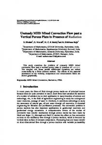
4. Results and Discussion The system of nonlinear differential equations (18) subject to boundary conditions (19) is solved numerically by the quasilinearization method. The influences of various fluid and geometric parameters such as Soret number Sr, Dufour number Du, Hartmann number Ha, chemical reaction parameter Kr, Schmidt number Sc, Eckert number Ec, and Prandtl number Pr on nondimensional velocity components, microrotation, temperature distribution, and concentration are analyzed through graphs in the domain [0, 1]. Figures 2 and 3 show the influence of Sr and Du on temperature and concentration. From these figures, it is

7

3

1.2

2.5

1

2

0.8

Concentration

Temperature


1.5 1

0.4 0.2

0.5 0

0.6

0 0

0.2

0.4

0.6

0.8

1

0

0.2

0.4

𝜆

Sr = 1 Sr = 1.5

Sr = 0.1 Sr = 0.5

0.6

0.8

1

𝜆

Sr = 1 Sr = 1.5

Sr = 0.1 Sr = 0.5

(a)

(b)

Figure 2: Effect of Sr on (a) temperature and (b) concentration for Kr = 2, Gr = 4, Gm = 4, Re = 2, Du = 2, Sc = 0.22, Pr = 1, 𝑎 = 0.2, 𝜓 = 0.2, 𝑅 = 0.2, 𝐽1 = 0.2, 𝑠1 = 2, 𝑠2 = 10, Ha = 1, 𝐷−1 = 2, and Ec = 1. 3.5

1.2

3

1 Concentration

Temperature

2.5 2 1.5 1

0.8 0.6 0.4 0.2

0.5

0

0 0

0.2

0.4

0.6

0.8

1

0

0.2

0.4

Du = 2 Du = 3

Du = 0.1 Du = 1

0.6

0.8

1

𝜆

𝜆

(a)

Du = 2 Du = 3

Du = 0.1 Du = 1 (b)

Figure 3: Effect of Du on (a) temperature and (b) concentration for Kr = 2, Gr = 4, Gm = 4, Re = 2, Sr = 1, Sc = 0.22, Pr = 1, 𝑎 = 0.2, 𝜓 = 0.2, 𝑅 = 0.2, 𝐽1 = 0.2, 𝑠1 = 2, 𝑠2 = 10, Ha = 1, 𝐷−1 = 2, and Ec = 1.

evident that the temperature of the fluid increases whereas the concentration decreases with the increasing of Sr and Du. This is because of the difference between the temperatures of the fluid and surface as well as the difference between concentrations of the fluid and surface concentrations are increased with Sr and Du. Figure 4 describes the behavior of the temperature distribution and concentration for the various values of Kr. As Kr increases the temperature distribution of the fluid also increases, whereas the concentration decreases from the lower plate to the upper plate. It is clear that the increase in the Kr produces a decrease in the species concentration. This causes the concentration buoyancy effects to decrease as Kr increases. The effect of Ec on velocity components, microrotation, and temperature is presented in Figure 5. As Ec

increases the radial velocity, microrotation and temperature are decreasing towards the upper plate. However, the axial velocity decreases towards the center of the channel and then increases. Since the Eckert number is the relation between the kinetic energy and enthalpy, as enthalpy increases, the temperature distribution decreases. Figure 6 elucidates the change in velocity components, microrotation, temperature distribution, and concentration for different values of Pr. It is observed that the axial velocity reaches highest value near the hot plate and the radial velocity, microrotation, and concentration decrease whereas the temperature increases with the increasing value of Pr. Physically, if Pr increases the thermal diffusivity decreases and this leads to the decrease in the heat transfer ability at the thermal boundary layer.

Journal of Engineering 1.8

0.8

1.6

0.7

1.4

0.6

1.2

Concentration

Temperature

8

1 0.8 0.6

0.5 0.4 0.3

0.4

0.2

0.2

0.1

0

0 0

0.2

0.4

0.6

0.8

1

0

0.2

0.4

0.6

𝜆

1

𝜆

Kr = 6 Kr = 8

Kr = 2 Kr = 4

0.8

Kr = 6 Kr = 8

Kr = 2 Kr = 4

(a)

(b)

Figure 4: Effect of Du on (a) temperature and (b) concentration for Du = 1, Gr = 4, Gm = 4, Re = 2, Sr = 0.2, Sc = 0.22, Pr = 1, 𝑎 = 0.2, 𝜓 = 0.8, 𝑅 = 2, 𝐽1 = 0.2, 𝑠1 = 2, 𝑠2 = 10, Ha = 2, 𝐷−1 = 2, and Ec = 1. 0.69

1

0.67

0.8

0.65

Radial velocity

Axial velocity

1.2

0.6 0.4

0.63 0.61 0.59

0.2

0.57 0.55

0 0

0.2

0.4

0.6

0.8

0

1

0.2

0.4

Ec = 1 Ec = 1.4

Ec = 0.2 Ec = 0.6

0.6

0.8

1

𝜆

𝜆

Ec = 1 Ec = 1.4

Ec = 0.2 Ec = 0.6

(a)

(b)

0.1

3.5

0.05

3

0

2.5

0

0.2

0.4

−0.05

0.6 𝜆

−0.1

0.8

1

Temperature

Microrotation

4

2 1.5 1

−0.15

0.5

−0.2

0 0

−0.25

0.2

0.4

0.6

0.8

1

𝜆

Ec = 1 Ec = 1.4

Ec = 0.2 Ec = 0.6 (c)

Ec = 1 Ec = 1.4

Ec = 0.2 Ec = 0.6 (d)

Figure 5: Effect of Ec on (a) axial velocity, (b) radial velocity, (c) microrotation, and (d) temperature for 𝐷−1 = 2, Du = 0.2, Gr = 4, Re = 2, Sr = 0.2, Ha = 2, Sc = 0.22, 𝑎 = 0.2, 𝜓 = 0.8, 𝑅 = 2, 𝐽1 = 2, 𝑠1 = 2, 𝑠2 = 1, Gm = 4, Kr = 2, and Pr = 0.71.


9 0.71

1.2

0.69

1 Radial velocity

Axial velocity

0.67 0.8 0.6 0.4

0.65 0.63 0.61 0.59

0.2

0.57 0.55

0 0

0.2

0.4

0.6

0.8

0

1

0.2

0.4

0.6

Pr = 0.2 Pr = 0.4

0.8

1

𝜆

𝜆

Pr = 0.71 Pr = 1

Pr = 0.71 Pr = 1

Pr = 0.2 Pr = 0.4

(a)

(b)

1.6 1.4

0.1

1.2

Microrotation

0.05 0 0

0.2

0.4

−0.05

0.6

0.8

1

Temperature

0.15

𝜆

1 0.8 0.6 0.4

−0.1

0.2

−0.15

0 0

−0.2

0.2

0.4

0.6

0.8

1

𝜆

Pr = 0.2 Pr = 0.4

Pr = 0.2 Pr = 0.4

Pr = 0.71 Pr = 1 (c)

Pr = 0.71 Pr = 1 (d)

0.7 0.6

Concentration

0.5 0.4 0.3 0.2 0.1 0 0

0.2

0.4

0.6

0.8

1

𝜆

Pr = 0.2 Pr = 0.4

Pr = 0.71 Pr = 1 (e)

Figure 6: Effect of Pr on (a) axial velocity, (b) radial velocity, (c) microrotation, (d) temperature, and (e) concentration for 𝐷−1 = 2, Du = 0.2, Gr = 4, Re = 2, Sr = 0.2, Ha = 2, Sc = 0.22, 𝑎 = 0.2, 𝜓 = 0.8, 𝑅 = 2, 𝐽1 = 0.2, 𝑠1 = 2, 𝑠2 = 1, Gm = 4, Kr = 2, and Ec = 1.

10


0.98

1.4

0.93 0.88 Radial velocity

Axial velocity

1.2 1 0.8 0.6

0.83 0.78 0.73

0.4

0.68

0.2

0.63

0 0.2

0

0.4

0.6

0.8

0.58

1

0

0.2

0.4

0.6

𝜆

Ha = 3 Ha = 4

Ha = 1 Ha = 2

0.8

1

0.8

1

𝜆

Ha = 3 Ha = 4

Ha = 1 Ha = 2

(a)

(b)

1.4 0.15

1.2

0.1

1 Temperature

Microrotation

0.05 0 −0.05

0

0.2

0.4

0.6

0.8

1

𝜆

0.8 0.6

−0.1

0.4

−0.15

0.2

−0.2

0 0

−0.25

0.2

0.4

0.6 𝜆

Ha = 3 Ha = 4

Ha = 1 Ha = 2

Ha = 3 Ha = 4

Ha = 1 Ha = 2

(c)

(d)

1 0.9 0.8 Concentration

0.7 0.6 0.5 0.4 0.3 0.2 0.1 0 0

0.2

0.4

0.6

0.8

1

𝜆

Ha = 3 Ha = 4

Ha = 1 Ha = 2 (e)

Figure 7: Effect of Ha on (a) axial velocity, (b) radial velocity, (c) microrotation, (d) temperature, and (e) concentration for Kr = 2, Du = 0.02, Gr = 4, Re = 2, Sr = 0.2, Sc = 1, Pr = 0.2, 𝑎 = 0.4, 𝜓 = 0.2, 𝑅 = 2, 𝐽1 = 2, 𝑠1 = 2, 𝑠2 = 2, Gm = 4, 𝐷−1 = 0.2, and Ec = 1.

Journal of Engineering Figure 7 displays the change in the velocity components, microrotation, temperature distribution, and concentration for several values of Ha. From this it is observed that when Ha increases, the temperature distribution also increases whereas the concentration decreases from the lower plate to upper plate and the axial velocity attains maximum value at the center of the plates. However, the radial velocity and microrotation increase towards the center of the plates and then decrease. This is due to the fact that the magnetic force retards the flow in both axial and radial directions. The variations in the velocity components, microrotation, temperature distribution, and concentration for different values of 𝐷−1 are shown in Figure 8. From these one can deduce that the temperature distribution is increasing with 𝐷−1 whereas the radial velocity, microrotation, and concentration are decreasing towards the upper plate and the axial velocity decreases towards the center of the plates and then increases because the resistance offered by the porosity of the medium is more than the resistance due to the magnetic lines of force.

5. Conclusions The thermal diffusion and diffusion thermoeffects on combined free and forced convection magnetohydrodynamic flow of micropolar fluid in a porous medium between two parallel plates with chemical reaction are considered. The numerical solution of the transformed governing equations is obtained by the method of quasilinearization and the results are analyzed for various fluid and geometric parameters through graphs. From the results the following is concluded: (i) The influences of Sr and Du on temperature and concentration are similar. (ii) The temperature of the fluid is enhanced whereas the concentration of the fluid is decreased with the increasing of Ha and 𝐷−1 .

11 𝑘1 : 𝑘2 : 𝑘3 : 𝑢: V: Pr: Re: 𝑗: 𝐽: 𝐽1 : 𝐵: 𝑏: 𝐵0 : 𝐷: 𝐸: Ha: 𝐷−1 : 𝑅: 𝑠1 : 𝑠2 : 𝑇: 𝑇1 𝑒𝑖𝜔𝑡 : 𝑇2 𝑒𝑖𝜔𝑡 : 𝑇∗ : 𝐶: 𝐶∗ : 𝐶0 𝑒𝑖𝜔𝑡 : 𝐶1 𝑒𝑖𝜔𝑡 : 𝐷1 : Kr:

(iii) Kr reduces the concentration and enhances the temperature of the fluid.

Sc: Gr:

(iv) Ec and Pr exhibit similar effects on the velocity components and microrotation whereas it is opposite in the case of temperature.

Gm:

Nomenclature 𝑎: 𝑡: ℎ: 𝑉1 𝑒𝑖𝜔𝑡 : 𝑉2 𝑒𝑖𝜔𝑡 : 𝑝: 𝑞: 𝑐: 𝑙: 𝑁: Ec: 𝑘:

Injection suction ratio, 1 − 𝑉1 /𝑉2 Time Distance between two parallel plates Injection velocity Suction velocity Fluid pressure Velocity vector Specific heat at constant temperature Microrotation vector Microrotation component Eckert number, 𝜇𝑉2 /𝜌ℎ𝑐(𝑇2 − 𝑇1 ) Thermal conductivity

Sh: 𝑛𝐴̇ : Sr: Du: 𝑇𝑚 : 𝑘𝑇 : 𝑐𝑠 :

Viscosity parameter Permeability of the medium Chemical reaction rate Velocity component in 𝑥-direction Velocity component in 𝑦-direction Prandtl number, 𝜇𝑐/𝑘 Suction Reynolds number, 𝜌𝑉2 ℎ/𝜇 Gyration parameter Current density Nondimensional gyration parameter, 𝜌𝑗ℎ𝑉2 /𝛾 Total magnetic field Induced magnetic field Magnetic flux density Rate of deformation tensor Electric field Hartmann number, 𝐵0 ℎ√𝜎/𝜇 Inverse Darcy parameter, ℎ2 /𝑘2 Nondimensional viscosity parameter, 𝑘1 /𝜇 Nondimensional micropolar parameter, 𝑘1 ℎ2 /𝛾 Nondimensional micropolar parameter, 𝛾𝑐/ℎ2 𝑘 Temperature Temperature of the lower plate Temperature of the upper plate Dimensionless temperature, (𝑇 − 𝑇1 𝑒𝑖𝜔𝑡 )/(𝑇2 − 𝑇1 )𝑒𝑖𝜔𝑡 Concentration Nondimensional concentration, (𝐶 − 𝐶0 𝑒𝑖𝜔𝑡 )/(𝐶1 − 𝐶0 )𝑒𝑖𝜔𝑡 Concentration of the lower plate Concentration of the upper plate Mass diffusivity Nondimensional chemical reaction parameter, 𝑘3 ℎ2 /𝐷1 Schmidt number, 𝜐/𝐷1 Thermal Grashof number, 𝜌𝑔𝛽𝑇 (𝑇2 − 𝑇1 )ℎ2 /𝜇𝑉2 Solutal Grashof number, 𝜌𝑔𝛽𝐶(𝐶1 − 𝐶0 )ℎ2 /𝜇𝑉2 Sherwood number, 𝑛𝐴̇ /ℎ𝜐(𝐶1 − 𝐶0 ) Mass transfer rate Soret number, 𝐷1 𝑘𝑇 𝜐𝑉2 /𝑐𝑇𝑚 𝑛𝐴̇ Dufour number, 𝐷1 𝑘𝑇 𝑛𝐴̇ 𝜌𝑐/𝜐2 𝑉2 𝑐𝑠 𝑘 Mean temperature Thermal diffusion ratio Concentration susceptibility.

Greek Letters 𝜆: 𝛼, 𝛽, 𝛾: 𝜁: 𝜐: 𝜌: 𝜇:

Dimensionless 𝑦 coordinate, 𝑦/ℎ Gyro viscosity parameters Dimensionless axial variable, (𝑈0 /𝑎𝑉2 − 𝑥/ℎ) Kinematic viscosity Fluid density Fluid viscosity

12


0.98

1.4

Radial velocity

Axial velocity

1.2 1 0.8 0.6

0.88

0.4 0.2 0.78

0 0

0.2

0.4

0.6

0.8

1

0

0.2

0.4

0.6

𝜆

0.8

1

𝜆

D−1 = 20 D−1 = 30

D−1 = 1 D−1 = 10

D−1 = 20 D−1 = 30

D−1 = 1 D−1 = 10

(a)

(b)

0.15

4

0.1

3.5

0.05

3

Temperature

Microrotation

4.5

0 −0.05

0

0.2

0.4

0.6

0.8

1

𝜆

−0.1

2.5 2 1.5

−0.15

1

−0.2

0.5

−0.25

0 0

−0.3

0.2

0.4

0.6

0.8

1

𝜆

D−1 = 20 D−1 = 30

D−1 = 1 D−1 = 10

D−1 = 20 D−1 = 30

D−1 = 1 D−1 = 10

(c)

(d)

1.2

Concentration

1 0.8 0.6 0.4 0.2 0 0

0.2

0.4

0.6

0.8

1

𝜆

D−1 = 20 D−1 = 30

D−1 = 1 D−1 = 10

(e)

Figure 8: Effect of 𝐷−1 on (a) axial velocity, (b) radial velocity, (c) microrotation, (d) temperature, and (e) concentration for Kr = 2, Du = 0.02, Gr = 4, Re = 2, Sr = 0.2, Ha = 1, Sc = 0.2, Pr = 0.2, 𝑎 = 0.2, 𝜓 = 0.2, 𝑅 = 2, 𝐽1 = 2, 𝑠1 = 2, 𝑠2 = 2, Gm = 4, and Ec = 1.

Journal of Engineering 𝜇󸀠 : Magnetic permeability 𝜎: Electric conductivity 𝜓: Nondimensional frequency parameter, 𝜔𝑡.

Conflict of Interests The authors declare that there is no conflict of interests regarding the publication of this paper.

Acknowledgments The authors thank referees for their suggestions which have resulted in the improvement of the paper. Also one of the authors (N. Naresh Kumar) is grateful to the Defence Research and Development Organization, Government of India, for providing senior research fellowship.

References [1] A. S. Berman, “Laminar flow in channels with porous walls,” Journal of Applied Physics, vol. 24, pp. 1232–1235, 1953. [2] R. M. Terril and G. M. Shrestha, “Laminar flow through parallel and uniformly porous walls of different permeability,” Zeitschrift f¨ur Angewandte Mathematik und Physik, vol. 16, pp. 470–482, 1965. [3] A. C. Eringen, “Theory of micropolar fluids,” Journal of Mathematics and Mechanics, vol. 16, pp. 1–18, 1966. [4] V. U. K. Sastry and V. Rama Mohan Rao, “Numerical solution of micropolar fluid flow in a channel with porous walls,” International Journal of Engineering Science, vol. 20, no. 5, pp. 631–642, 1982. [5] O. Ojjela and N. Naresh Kumar, “Unsteady MHD flow and heat transfer of micropolar fluid in a porous medium between parallel plates,” Canadian Journal of Physics, vol. 93, no. 8, pp. 880–887, 2015. [6] D. Srinivasacharya, J. V. Ramana Murthy, and D. Venugopalam, “Unsteady stokes flow of micropolar fluid between two parallel porous plates,” International Journal of Engineering Science, vol. 39, no. 14, pp. 1557–1563, 2001. [7] G. Maiti, “Convective heat transfer in micropolar fluid flow through a horizontal parallel plate channel,” ZAMM—Journal of Applied Mathematics and Mechanics, vol. 55, no. 2, pp. 105– 111, 1975. [8] R. Bhargava, L. Kumar, and H. S. Takhar, “Numerical solution of free convection MHD micropolar fluid flow between two parallel porous vertical plates,” International Journal of Engineering Science, vol. 41, no. 2, pp. 123–136, 2003. [9] M. Ashraf and A. R. Wehgal, “MHD flow and heat transfer of micropolar fluid between two porous disks,” Applied Mathematics and Mechanics, vol. 33, no. 1, pp. 51–64, 2012. [10] A. Islam, Md. H. A. Biswas, Md. R. Islam, and S. M. Mohiuddin, “MHD micropolar fluid flow through vertical porous medium,” Academic Research International, vol. 1, no. 3, pp. 381–393, 2011. [11] S. Nadeem, M. Hussain, and M. Naz, “MHD stagnation flow of a micropolar fluid through a porous medium,” Meccanica, vol. 45, no. 6, pp. 869–880, 2010. [12] O. Ojjela and N. Naresh Kumar, “Unsteady heat and mass transfer of chemically reacting micropolar fluid in a porous

13 channel with hall and ion slip currents,” International Scholarly Research Notices, vol. 2014, Article ID 646957, 11 pages, 2014. [13] N. S. Elgazery, “The effects of chemical reaction, Hall and ion-slip currents on MHD flow with temperature dependent viscosity and thermal diffusivity,” Communications in Nonlinear Science and Numerical Simulation, vol. 14, no. 4, pp. 1267–1283, 2009. [14] M. S. Ayano, “Mixed convection flow micropolar fluid over a vertical plate subject to hall and ion-slip currents,” International Journal of Engineering & Applied Sciences, vol. 5, no. 3, pp. 38– 52, 2013. [15] A. R. M. K. Aurangzaib, N. F. Mohammad, and S. Shafie, “Soret and dufour effects on unsteady MHD flow of a micropolar fluid in the presence of thermophoresis deposition particle,” World Applied Sciences Journal, vol. 21, no. 5, pp. 766–773, 2013. [16] D. Srinivasacharya and C. RamReddy, “Soret and Dufour effects on mixed convection in a non-Darcy porous medium saturated with micropolar fluid,” Nonlinear Analysis: Modelling and Control, vol. 16, no. 1, pp. 100–115, 2011. [17] A. Mahdy, “Soret and Dufour effect on double diffusion mixed convection from a vertical surface in a porous medium saturated with a non-Newtonian fluid,” Journal of Non-Newtonian Fluid Mechanics, vol. 165, no. 11-12, pp. 568–575, 2010. [18] T. Hayat and M. Nawaz, “Soret and Dufour effects on the mixed convection flow of a second grade fluid subject to Hall and ionslip currents,” International Journal for Numerical Methods in Fluids, vol. 67, no. 9, pp. 1073–1099, 2011. [19] H. P. Rani and C. N. Kim, “A numerical study of the dufour and soret effects on unsteady natural convection flow past an isothermal vertical cylinder,” Korean Journal of Chemical Engineering, vol. 26, no. 4, pp. 946–954, 2009. [20] D. Pal and H. Mondal, “Effects of Soret Dufour, chemical reaction and thermal radiation on MHD non-Darcy unsteady mixed convective heat and mass transfer over a stretching sheet,” Communications in Nonlinear Science and Numerical Simulation, vol. 16, no. 4, pp. 1942–1958, 2011. [21] B. K. Sharma, K. Yadav, N. K. Mishra, and R. C. Chaudhary, “Soret and Dufour effects on unsteady MHD mixed convection flow past a radiative vertical porous plate embedded in a porous medium with chemical reaction,” Applied Mathematics, vol. 3, no. 7, pp. 717–723, 2012. [22] E. S. Lee and L. T. Fan, “Quasilinearization technique for solution of boundary layer equations,” The Canadian Journal of Chemical Engineering, vol. 46, no. 3, pp. 200–204, 1968. [23] T. Hymavathi and B. Shanker, “A quasilinearization approach to heat transfer in MHD visco-elastic fluid flow,” Applied Mathematics and Computation, vol. 215, no. 6, pp. 2045–2054, 2009. [24] C. L. Huang, “Application of quasilinearization technique to the vertical channel flow and heat convection,” International Journal of Non-Linear Mechanics, vol. 13, no. 2, pp. 55–60, 1978. [25] S. S. Motsa, P. Sibanda, and S. Shateyi, “On a new quasilinearization method for systems of nonlinear boundary value problems,” Mathematical Methods in the Applied Sciences, vol. 34, no. 11, pp. 1406–1413, 2011. [26] R. E. Bellman and R. E. Kalaba, Quasilinearization and Boundary-Value Problems, Elsevier, New York, NY, USA, 1965.

International Journal of

Rotating Machinery

Engineering Journal of

Hindawi Publishing Corporation http://www.hindawi.com

Volume 2014

The Scientific World Journal Hindawi Publishing Corporation http://www.hindawi.com

Volume 2014


Distributed Sensor Networks

Journal of

Sensors Hindawi Publishing Corporation http://www.hindawi.com

Volume 2014


Volume 2014


Volume 2014

Journal of

Control Science and Engineering

Advances in

Civil Engineering Hindawi Publishing Corporation http://www.hindawi.com


Volume 2014

Volume 2014

Submit your manuscripts at http://www.hindawi.com Journal of

Journal of

Electrical and Computer Engineering

Robotics Hindawi Publishing Corporation http://www.hindawi.com


Volume 2014

Volume 2014

VLSI Design Advances in OptoElectronics


Navigation and Observation Hindawi Publishing Corporation http://www.hindawi.com

Volume 2014



Chemical Engineering Hindawi Publishing Corporation http://www.hindawi.com

Volume 2014

Volume 2014

Active and Passive Electronic Components

Antennas and Propagation Hindawi Publishing Corporation http://www.hindawi.com

Aerospace Engineering


Volume 2014


Volume 2014

Volume 2014




Modelling & Simulation in Engineering

Volume 2014


Volume 2014

Shock and Vibration Hindawi Publishing Corporation http://www.hindawi.com

Volume 2014

Advances in

Acoustics and Vibration Hindawi Publishing Corporation http://www.hindawi.com

Volume 2014