WEST-EAST HIGH SPEED FLOW FIELD CONFERENCE 19-22, November 2007 Moscow, Russia
UNSTRUCTURED MESHES IN UNSTEADY CFD APPLICATIONS Dmitry A. Lysenko Engineering Technology Center, ETEC GE Energy Masterkova str.4, 17th floor, 115280 Moscow, Russia Email:
[email protected], web page: http://www.ge.ru
Key words: CFD, structured/unstructured grids, turbulent separated compressible/incompressible flows, parallel computing, Euler/URANS/LES methods. Abstract. Four state-of-the-art applications of unstructured tetrahedral meshes (both static and dynamicadaptive) in numerical simulations of different fluid dynamics phenomena are presented. The numerical methods are varied form simple Euler equations through unsteady Reynolds averaged equations to filtered Navie-Stokes equations. Meshes practically of all types are applied for these simulations. Special attention is devoted to the questions related to dynamic adaptive grids for unsteady flows. Overall, it’s shown that unstructured grids are highly competitive with traditional structured meshes.
1.
INTRODUCTION
High efficiency generation of unstructured grids for objects with complicated geometry together with violence increasing of computer’s power and development of powerful effective numeric methods allow to conduct more and more complex CFD investigations in different areas of hydro- and aerodynamics. As a result, the question of adequacy using of such meshes in numerical simulations is coming up. The effective usage and numerical accuracy obtained on such meshes are presented based on fundamental fluid flow’s test cases, such as: 1) laminar flow over a circular cylinder1 (Reynolds number, Re = 140), for the purpose of reproduction in a numerical experiment - visualization of a Karman vortex street (presented in the known Van Dyke atlas of flows) by smoke; 2) supersonic flow in the step channel2 with Mach number, M = 3 where the degree of resolution of complex aerodynamics elements and phenomena – the unsteady interaction of compression and rarefaction and Mach disks occurring in interaction of shock waves with each other and with the walls – with the use of selected numerical algorithm are of special interest; 3) turbulent supersonic flow around 2D wedge-plate model3 (M = 2) results in the generation of a complex flow downstream of the body, characterized by a large separated region bounded by separating free shear layers and the base wall. Because the near wake region influences the performance of many fluid dynamic applications there is a strong motivation to better understand its fundamental features from the numerical and experimental point of view; 4) fully developed turbulent channel flow around a single surface-mounted cubical obstacle4,5
D. LYSENKO/Unstructured meshes in unsteady CFD applications
(Re = 40,000). The separated region in front of the cube is characterized by the appearance of a quasi-regular distribution of saddle and nodal points on the forward face. These three-dimensional effects are considered to be inherent to such separating flows with stagnation. Several different approaches are applied to predict governmental fluid flow equations implemented in CFD code FLUENT v6.2-6.3 which are varied from Euler equations through unsteady Reynolds averaged equations to filtered Navie-Stokes equations.
2.
PARALLEL COMPUTING
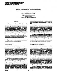
Analyzing data located on the site of Top500 project6 which are used in forming of the most powerful supercomputer’s list (Figure 1) one can make an estimation that parallel computers will achieve a PentaFlops performance at least in 2010 year. The Top500 list is forming according to results based on famous test Linpack7. Besides theoretical performance (Rpeak) additionally Rmax (obtained in Linpack with the maximum for a given computer system matrix – Nmax) value is pointed for each system. The final list is sorted according to the Rmax values. Figure 1 illustrates a quite optimistic trend in performance increasing both for parallel (1,2) and personal (4,5) computer systems.
Figure 1. Computer’s performance evolution. (1) – parallel computers and its trend line (2); (3) – target performance; (4) – personal computers based on Intel CPU’ and its trend line (5).
Especially this tendency looks optimistic for cluster systems, which can be considered as the most economical and high-productivity computational systems for engineering and scientific simulations. Another interesting observations following from Figure 1 consists of the fact that interpolations (2) and (5) parallel to each other. And it’s not surprised because parallel and personal computers have the same component base. Testing of the CFD code FLUENT8 based on 4-nodes Linux-cluster system (with the following node configuration: HP DL360, 2x Intel Xeon 3GHz, 4 GB Memory, 1G-T network) shown the performance’s increasing in 6.76 times, compare to 8 times in an ideal case. Official data presented on the FLUENT company web-site shown the result
D. LYSENKO/Unstructured meshes in unsteady CFD applications
of 6.88 performance’s increasing for the systems with similar configurations9. The test was performed for turbulent separation flow in the channel with the grid size of 1.3M nodes. From several available algorithms of fluid flow equations modeling the “worst” segregated approach was chosen. In this case the government equations are solving sequentially (another method represents coupled solution) i.e. the pressure-velocity coupling (or SIMPLEC based) method is used. Thus, when equations are nonlinear and independent it’s needed to perform additional sub-iterations to get the convergence on each iteration step. In such a way an additional load is taken place on the network hardware because information exchange between computational nodes is increasing significantly.
3.
LAMINAR FLOW AROUND A CIRCULAR CYLINDER
Methodical investigation of an unsteady laminar flow around a circular cylinder at a definite Reynolds number (Re = 140) was carried out for the purpose of reproduction, in a numerical experiment, of the physical conditions of visualization of a Karman vortex shedding (presented in the known Van Dyke atlas of flows10) by smoke1. A smoke jet introduced into an air flow passes around the circular cylinder and colors the vortex flow in the wake. This problem on a two-phase flow around a body is solved on unstructured triangular grid adapted to the CO concentration. The computational region represents a rectangle of size 6.5 × 2 m. A cylinder of diameter 0.1 m is located at a distance of 17.5 calibers from the input boundary and symmetrically relative to the upper and positioned boundaries. The width of the gas jet supplied is 0.01 m (10% of the cylinder diameter). The simulation is carried out based on unstructured triangular grid (Figure 1a). A structured ring grid with a minimum nearwall step of 10-5 m surrounds the cylinder. The cylinder profile is divided into 100 equal intervals. The grid is adapted to three regions: 1) a circle of radius 0.5 m, the center of which coincides with the center of the cylinder; 2) a rectangular region of size 4.65 × 1.2 m, used for better representation of the wake formed downstream of the cylinder; 3) a rectangular region of size 1.75 × 0.4 m, used for better representation of the zone where the air flows are mixed with the smoke jet. The time step is taken to be equal to 0.1 sec. A gas mixture of air with smoke contains O2, N2, and CO. The mixture’s density and viscosity are calculated according to volume-weighted-mixing-law8 and to massweighted-mixing-law8. The inlet boundary conditions are defined by the velocities of the flows and the mass fractions of the components (0.23 for O2 and 1 for CO). The velocity of the incoming flow is determined at a definite value of the Reynolds number (Re = 140). The symmetry conditions are set at the upper and lower boundaries of the computational region. Outflow conditions are set at the output boundary. A system of URANS equations and transport equations of gas-mixture components are solved by the factorized finite-difference method based on algebraic multigrid method11. The computational algorithm involves the third-order approximation of the convective terms in equations by the QUICK scheme12, the second-order approximation of the pressure13, the PISO procedure of pressure correction14, and the second-order discretization with respect to time by an implicit iterative scheme15. Particular emphasis is placed on the triangular grids (Figure. 2a) adapted to the solution of the problem (the CO concentration), because these grids are best suited for representation of details of the vortex structure of a flow around a cylinder. This is explained by the fact that the density of cells in them is larger where this is desired, i.e.,
D. LYSENKO/Unstructured meshes in unsteady CFD applications
in the zones of vortex cores. Nonetheless, despite the high accuracy of reproduction of the pattern of a flow and the minimum errors in the solution, only a grid containing an extremely large number of cells (as large as 1,500,000) can be adapted to a solution.
Figure 2. Unstructured triangular grid (a) with local dynamic refinement with respect to the CO concentration. Comparison of the smoke concentration (b): measured (1) and calculated (2) at Re = 140; data (1) was taken from Van Dyke atlas10.
It is known that a Karman vortex street is formed in the wake downstream of the cylinder; a smoke jet easily visualizes it at small velocities of the flow, e.g. The positions of the vorticity bunches correspond to the positions of the smokeconcentration cores numerically calculated and the cores presented on the photograph of a flow visualized by smoke at Re = 140, taken from the Van-Dyke atlas10. The trajectory of a fluid particle, moving from the separation region to the cylinder, passes through the centers of the bunches and/or concentration cores and has a wave-like shape. It is also significant that the Strouhal number (Sh = 0.172) calculated at Re = 140 is in good agreement with measured values16,17.
4.
A MACH 3 WIND TUNNEL WITH A STEP
The problem on supersonic flow in a channel with a step for Mach number M = 3 has been a popular test for comparison of the accuracy of different computational schemes and methods over many years. It was introduced more then fifty years ago by Emery18, but it overall public acknowledgement was taken place after paper by Woodward and Colella in 198419. Thus, this problem has proven to be useful test for a large number of numerical methods, schemes and algorithms during large number of years. Of special interest is the degree of resolution of complex aerodynamics elements and phenomena – the nonstationary interaction of compression and rarefaction and Mach disks occurring in interaction of shock waves with each other and with the walls – with the use of selected numerical algorithm. The wind tunnel is 1 length unit wide and 3 length unit long. The step is 0.2 length units high and is located 0.6 length units from the left-hand end of the tunnel. It’s assumed here that tunnel has an infinity width, or in other words it’s considered two-dimensional planar base flow. The test has the following boundary conditions: flow inlet conditions
D. LYSENKO/Unstructured meshes in unsteady CFD applications
at the felt (basically so-called pressure-inlet conditions are used) and at the right all gradients are assumed to vanish. Since the exit velocity is always supersonic the exit boundary conditions has no effect on the flow. Along the walls of the tunnel reflecting boundary conditions are applied. Initially wind tunnel is filled with a inviscid γ-law (or ideal) gas (γ = 1.4), which everywhere has density 1.4, pressure 1.0 and axial velocity 3. Gas with such properties is continually fed in from the left-hand boundary. The corner of the step is the center of rarefaction fan and hence is a singular point of the flow. Frankly speaking the flow is seriously affected by large numerical errors generated just in the neighborhood of this singular point if nothing special is not undertaken. The modern study shown that the presence of such point in flow may lead to phase – time delay20. In general, there are two ways to reduce or eliminate this point. The original idea was proposed by Woodward19 and consisted of applying special boundary conditions near the corner of the step, which is based on the assumption of a nearly steady flow in this region. The density was reset here so that the entropy had the same value as in the zone just to the left and below the corner of the step. The magnitudes of velocities (but no their directions) were reset also, so that the sum of enthalpy and kinetic energy per unit mass had the same value as in the same zone to set the entropy. More sophisticated and accurate approach may be applied to solve this problem, which consists in making a little fillet to avoid the straight angle in the step corner. Robust unstructured meshes allow additionally preparing some grid refinement in this region. It was shown previously20 that either structured or unstructured meshes allow obtaining quite good results regarding this test problem. In this paper uniform triangular grid was used with the size of element equal to 0.0125 – which one may consider equivalent to the quad structured grid with the element size19: Δx = Δy = 1/80. Compare to previous results20 the number of grid nodes was increased from 8 to 20 thousands. Insignificant mesh refinement is performed in the area of the singular point. This mesh is used also as initial for numerical simulations with dynamic local grid adaptation based on the density field with two levels of refinement. During simulations the total number of elements is limited by 400 thousands, the control values for mesh refinement and coursing are set as 0.01 and 0.02 respectively. Domain remeshing is occurred after each 5 time steps. The finite-volume method based on the conception of precondition technique21 is used to solve Euler equations. Modified Advection Upstream Splitting Method22,23 for inviscid flux-difference splitting and the standard second order accuracy upwind scheme for convective terms calculations24 are applied. The implicit-time stepping (also known as dual-time formulation) based on second order Euler backward method is used for time integration25. Inner iterations in pseudo-time are performed based on implicit timemarching scheme26. CFL condition is set to 0.8 for this case and unsteady simulations are carried out with fixed time-step equal to 0.0025.
D. LYSENKO/Unstructured meshes in unsteady CFD applications
Figure 3. Numerical results performed with dynamic local-gradient mesh refinement for time t= 4: dynamic unstructured triangular mesh (а); 30 equally spaced contours of log density (b), min and max values –1 and 1, respectively; 30 equally spaced contours of the numerical noise, min and max values 0.3 and 1.7, respectively (c).
Typical solution for time t = 4 based on dynamic local-gradient refinement is displayed in Figure 3: (a) – dynamic unstructured triangular mesh; (b) – contours of log density; (c) – contours of the quantity
(numerical noise), which is a function of
entropy. Main discordance, which should be underlined - Kelvin-Helmholtz instability development starting from the trinity point - intersection of the main strong shock wave and upper Mach disk. Such instabilities evolution is amplified by numeric errors generated in the trinity point while shock waves interaction independently of mesh density. Thus, promising for further investigation of this test may be switching from inviscid Eulers methods to viscous RANS approaches.
5.
TURBULENT SUPERSONIC FLOW AROUND THE 2D WEDGE-PLATE MODEL
The supersonic flow about a blunt-based body results in the generation of a complex flow downstream of the body, characterized by a large separated region bounded by separating free shear layers and the base wall. Because the near wake region influences the performance of many fluid dynamic applications, such as high-speed projectiles, missiles and bullets, there is a strong motivation to better understand its fundamental features from the numerical and experimental point of view. At present PIV (Particle Image Velocimetry) and POD (Proper Orthogonal Decomposition) methods are widely used to investigate turbulent transonic and supersonic planar compressible base flows to
D. LYSENKO/Unstructured meshes in unsteady CFD applications
obtain mean and instantaneous velocity fields in separation regions downstream of bluff-body27,28. From the other hand the modern CFD codes give a wide robust numerical methods for the prediction of the near wake region for such types of flows. Because the near wake region is dominated by intense velocity and density gradients due to the viscous action in the free shear it’s important to predict impact of turbulent viscosity during numerical simulations. It’s leads to use RANS/URANS methods (compressible Navier-Stokes equations) based on one of the turbulent closure assumptions instead of simple Euler approach. To demonstrate the correlation between abilities of modern experimental27,28 and state-of-the-art numerical methods8 the case of turbulent supersonic flow around the 2D wedge-plate model is chosen. Physical experiments were performed in the blow-down transonic-supersonic wind tunnel (TST-27) of the High-Speed Aerodynamics Laboratories at Delft University of Technology29 with a test section of 27 × 28 cm2. The facility generated flows in the Mach number range 0.5 to 4.2 in the test section, operating at unit Reynolds numbers ranging from 38×106 to 130×106 (m-1). The model consists of a symmetrical doublewedge with a sharp leading edge giving a deflection angle of 11.31 deg, followed by a 50mm long plate with constant base height thickness of h = 20mm. Based on these dimensions the total chord of the model was 100 mm. The model terminates with a vertical base and spans the width of the test section. The wind tunnel was operated at a stagnation pressure of approximately 200kPa. The tunnel operation was set to provide freestream Mach numbers of 2.0 (490m/s) respectively along the thick plate. Twocomponent PIV was employed. The PIV measurement consisted of 500 instantaneous snapshots returning the velocity distribution over the wake flow. The data sets were analyzed statistically returning the mean velocity pattern and the turbulence intensity spatial distribution. The implicit finite-volume method based on the conception of precondition technique21 is used to solve compressible RANS equations. Spalart-Allmaras turbulence model30 with rotation correction31,32 is applied for equation’s closure. AUSM22,23 for inviscid flux-difference splitting and standard upwind scheme of second order accuracy for convective terms calculations24 are used. The test has the following boundary conditions: flow inlet conditions at the felt (pressure-inlet) and at the right all gradients are assumed to vanish. Inlet flow had the following turbulence intensity and turbulence length scale: 3% and 0.02 m. Since the exit velocity is always supersonic the exit boundary conditions has no effect on the flow. Along the walls of the tunnel slipping boundary conditions are applied. The walls of the wedge-plate model have no-slip conditions. Initially wind tunnel is filled with an air with γ-law equation of state (γ = 1.4), which everywhere had total pressure 200 kPa, total temperature 270K, and Mach number M = 2. Gas with such properties is continually fed in from the left-hand boundary. Properties of the gas, such as heat capacity and viscosity are modeled using functional dependences of temperature8 (polynomial and Sutherland laws, respectively).
D. LYSENKO/Unstructured meshes in unsteady CFD applications
Figure 4. Unstructured triangular mesh (a) and 40 equally spaced contours of log density (b).
2D computational domain is chosen in such a way to replicate the conditions of TST-27 wind tunnel (Figure 4a). The length and the width of domain are: 1 m and 0.27 m, respectively. The wedge-plate bluff body is placed at the distance of 0.3 m from the inlet (left) boundary. The unstructured triangular mesh with total number cells of 171 K (~ 90K nodes) is used. The size of elements for bluff-body walls is chosen as 0.5 mm. Outer domain boundaries are meshed with the element’s size of ~7 mm with the purpose to provide the smooth transition in the grid cell sizes. The viscous structured sublayer is applied also to the walls of the wedge-plate body (first row size – 0.01 mm, growth factor – 1.5 and number of rows – 6). Thus the maximum Y+ value is received as 8.83. The general view of the computational domain with triangular grid is presented on Figure 4a. Figures 4-6 present some results. Contours of log density in the whole computational domain are shown in Figure 4b. The more detailed flow visualization near the bluffbody is presented in Figure 5. Schlieren image obtained in experiment (Figure 5a) is compared to numerically predicted density field (Figure 5b). Two-dimensional compressible flow features are clearly revealed by both methods: front shock (1), shoulder (2) and base (3) expansion fans emanating from the shoulder and base corners, shear layer (4) and the recompression waves (5). One can see the excellent match between experimental and numerical flow visualization. The near wake region is shown in Figure 6. The mean velocity distribution also provides the description of the separated shear layers (1), reverse flow (2), reattachment (3) and wake development (4). The streamlines verify the symmetry of the mean topology. Using these streamlines, the mean flow reattachment location is estimated to occur at approximately x/h= 1.25 respectively, consistent with previous related studies33 and current numerical results (Figure 6b).
D. LYSENKO/Unstructured meshes in unsteady CFD applications
Figure 5. Flow visualization near the wedge-plate bluff body: (a) – PIF method, (b) – numerical results, contours of density. Flow features: (1) - front shock (1), shoulder (2) and base (3) expansion fans emanating from the shoulder and base corners, shear layer (4) and the recompression waves (5).
Figure 6. Near wake zone downstream the bluff-body visualization: (a) – PIF method, (b) – numerical results (contours of density and streamlines).
6.
FULLY DEVELOPED TURBULENT FLOW AROUND A SURFACE MOUNTED CUBE IN THE CHANNEL
Large eddy simulation is applied for investigating well-known fully developed turbulent flow in the channel around a surface mounted cube34,35 with typical Reynolds number, Re = 40,000 (based on cubical obstacle size). Computational domain is selected from conditions of physical tests34,35. The cube side size D = 0.025 m is chosen as main length scale. Based on it, the height of the channel is equal to 2D, the length of the computational domain in the longitudinal direction is -
D. LYSENKO/Unstructured meshes in unsteady CFD applications
10D, the width (in transversal direction) - 4D, and the cube is mounted on the distance of 3D from the inlet boundary. The experimental turbulent velocity profile is applied at the inlet boundary. The mean inflow velocity magnitude is chosen as the dimensionless quantity with numeric value34,35 of 19.18 m/sec. Inlet turbulent intensity is set to 1.5% and the cube side size is taken as turbulent length scale. Outlet boundary conditions are treated as outflow; symmetry conditions - for lateral sides and the no-slip conditions for the cube and channel walls. The fluid is considered as incompressible and adiabatic. Both structured (hexahedral) and unstructured (tetrahedral) grids are used to estimate solution’s mesh independence. The structured mesh contains total number of nodes ~ 1.7M [278x112x56]. Exponential distribution of the nodes from the outside boundaries towards the cube is performed with the growth factor 0.8. Three unstructured tetrahedral grids are used additionally to assess the solution accuracy with the ratio of grid spacing (h) between each other’s of ~1.25, i.e. h2/h1 = h3/h2 ~ 1.25. Each tetrahedral mesh has the viscous boundary layer (number of rows – 6, the height of the first cell - 8х10-4 and growth factor − 1.9) and the same as for structured exponential distribution of the nodes from the outside boundaries towards the cube. Table 1 contains the grid’s information summary and the extreme values of the Y+ also. Method LES LES LES LES
Node's Mesh type number Hexa 1,776,627 Tetra 212,344 Tetra 382,244 Tetra 655,644
Cell's number 1,721,664 883,981 1,727,464 3,078,224
Y+ min 0.323 0.087 0.061 0.070
Y+ max 14.770 1.753 1.489 1.594
Time step 3.84E-03 7.67E-03 7.67E-03 7.67E-03
Table 1. Used meshes description.
Large-eddy simulation is based on implicit filtering of NS equations using top-hat filter36 and dynamic Smagorinsky-Lilly SGS model37,38. Thus, sub- grid resolution (the ratio of the filter width to the grid-spacing) is limited and equaled to 1. Second order upwind scheme for pressure24, bounded center-differencing scheme39 for all other convective terms, implicit non-iterative second order time integration scheme40 are used. Special inlet boundary conditions based on so-called vortex method41 are applied to inflow boundaries to simulate fluctuations of velocity field. The sampling data interval is chosen based on the assumption of ergodic’s theorem correctness42. It’s known, that ergodic’s theorem guarantees the match between time averaged and sampling averaged values under certain assumptions. To estimate the time period the so-called integral time scale is introduced (T* - the ratio between length scale and the typical velocity scale). It’s shown42 that the error is minimum when the sampling data interval significantly increased the integral time scale. For this problem, T* = 0.00125 sec., and sampling data is chosen ~ 0.1- 0.3 sec., respectively. The fixed time step is set in such manner to satisfy CFL conditions, i.e. the local Courant number has to be less the 1 in all computational domain. Some results related to the adequacy assess of the used grids are displayed on Figure 7. As the main comparison criteria time-averaged local profiles of the mean axial velocity are chosen in the center longitudinal section of the domain (z = 0). Some observations are outlined below. Figure 7a represents distributions of experimental data (1) and numerical results obtaining for hexahedral (2) and tetrahedral (3 – with number of cells ~ 1.7M) meshes. Figure 7b demonstrates solution independence obtaining on
D. LYSENKO/Unstructured meshes in unsteady CFD applications
unstructured tetrahedral meshes. One can see that increasing of the number of cells from 0.8M to 3.0M doesn’t affect on the solution significantly in case of unstructured meshes. In this case the match between solutions for all three unstructured grids are quite good. From the other side, looking on the distributions of experimental data and numerical results received on different mesh’s types (Figure 7a), it may be layout that some discrepancies between numerical solutions exist. First of all, the nature of them may be associated with simple geometry discretization principles. In general, if it’s needed to achieve the same approximation accuracy of one hexahedral cell it’s required about 6-8 tetrahedral cells. Thus, to compare ‘identical’ or ‘equal’ structured and unstructured grids between each other one has to keep the correlation between total number of nodes ~ 1:6. For example, if the structured hexahedral mesh contains about 1M cells, the ‘equal’ unstructured mesh must has at least ~6M cells. Since it is still quite computationally expensive to carry out LES on grids with such mesh density (>6M) this is a challenging task for the nearest future.
Figure 7. Adequacy assesses of the used grids based on time-averaged four local profiles of the mean (time-averaged) axial velocity in the center longitudinal section (z = 0): (a) – Distributions of experimental data (1) and numerical results obtaining for hexahedral (2) and tetrahedral (3 – with number of cells ~ 1.7M) meshes; (b) – unstructured meshes of levels 1-3, respectively.
Figure 8 demonstrates the time-averaged flow field with path lines in the central longitudinal section of the domain (z = 0): numerical results obtained on structured (a) and unstructured (b – with number of cells ~1.7 M) meshes, respectively; experimental oil-flow visualization (c). The integral values of separation and reattachment points (Xl and Xr on Figure 8, respectively) are given in Table 2. In the same place experimental values and the results of other authors are presented.
D. LYSENKO/Unstructured meshes in unsteady CFD applications
Figure 8. Time-averaged flow field in the central longitudinal section of the domain (z =0): numerical results obtained on structured (a) and unstructured (b) meshes and experimental oil-flow visualization (c). Contribution Martinuzzi and Tropea Breuer et al. Rodi et al. Shah Krajnovic & Davidson Present Calculations:
Year 1993 1997 1998 1999
Model Experiment LES LES LES LES
XF/D 1.04 1.23 1.00 1.08 1.06
XR/D 1.61 1.70 1.43 1.69 1.38
2007 2007
LES (Hexa) LES (Tetra)
0.84 1.12
1.62 1.72
Table 2. Integral parameters of the flow: numerical and experimental results.
7.
SUMMARY
There is the list of conclusions, which can be done from this study. •
High numerical accuracy of the 4 predicted state-of-the-art solutions (laminar flow around circular cylinder, a mach 3 wind tunnel with a step, turbulent supersonic flow around wedge-plate model, fully developed turbulent flow around a surfaced mounted cube in a channel) with unstructured meshes usage is demonstrated. Three different approaches are applied to model governmental fluid flow equations: Euler equations, RANS/URANS equations and filtered NS equations with two corresponded finite-volume methods based on pressurevelocity coupling11 and on the conception of precondition technique21, respectively.
D. LYSENKO/Unstructured meshes in unsteady CFD applications
•
All applied numerical methods are well validated and tested. Demonstrated in this article test cases may be used also to confirm it as all of them contain available experimental data and numerical results obtained by the different authors. Additionally all presented solutions were obtained both on structured and unstructured grids verifying the mesh independent data.
•
Overall, it’s shown based on presented results that unstructured grids are highly competitive with traditional structured meshes. A good match is obtained for all test cases in terms of mesh independence, adequacy of numerical and physical experimental results and also good correlations with others.
•
Local dynamic grids with gradient adaptation are powerful tool in unsteady simulations, though they are not used widely in industrial engineering calculations. It’s allowed significantly decrease the total CPU time and increased dramatically the solutions accuracy for the single CPU computers. But the main constraint in their wide applications is parallel computations. The advantage in efficiency of dynamic grids is becoming not so evident since it’s required to rebuild mesh on each time step.
8.
REFERENCES
[1]
S. A. Isaev, P. A. Baranov, N. A. Kudryavtsev, D. A. Lysenko, A. E. Usachev, “Comparative analysis of the calculation data on an unsteady flow around a circular cylinder obtained using the VP2/3 and FLUENT packages and the Spalart-Allmaras and Menter turbulence models”, Journal of Engineering Physics and Thermophysics, Vol:78(6)., 1199-1213 (2005).
[2]
S.A. Isaev., D.A. Lysenko, “Testing of the FLUENT package in calculations of supersonic flow in a step channel”, Journal of Engineering Physics and Thermophysics. Vol:77(4)., 857-860 (2004).
[3]
R.A. Humble, F. Scarano, B.W. van Oudheusden, “Application of PIV and POD to Unsteady Planar Base Flows”, PIVNET II International Workshop on the Application of PIV in Compressible Flows, (2005).
[4]
R. Martinuzzi, C. Tropea, “The flow around surface-mounted, prismatic obstacles placed in a fully developed channel flow”, Journal of Fluid Engineering, Vol. 115, 85-92 (1993).
[5]
http://cfd.me.umist.ac.uk/ercoftac/index.html.
[6]
www.top500.org
[7]
J. Dongarra, J.R. Bunch, C.B. Moler, G.W. Stewart, LINPACK User Guide, SIAM Publications, Philadelphia (1978).
[8]
Fluent Inc. Fluent 6.2. Users Guide. Lebanon (2004).
[9]
http://www.fluent.com/software/fluent/fl5bench/relinfo.htm
[10] M. Van Dyke, An Album of Fluid Motion [Russian translation], Mir, Moscow (1986). [11] B.R. Hutchinson, G.D. Raithby, A Multigrid Method Based on the Additive Correction Strategy. Numerical Heat Transfer, 9, 511-537 (1986).
D. LYSENKO/Unstructured meshes in unsteady CFD applications
[12] B.P. Leonard, S. Mokhtari, ULTRA-SHARP Nonoscillatory Convection Schemes for High-Speed Steady Multidimensional Flow. NASA TM 1-2568 (ICOMP-9012), NASA Lewis Research Center (1990). [13] T.J. Barth, D. Jespersen, The design and application of upwind schemes on unstructured meshes. Technical Report AIAA-89-0366, AIAA 27th Aerospace Sciences Meeting, Reno, Nevada (1989). [14] I R. Issa, Solution of Implicitly Discretized Fluid Flow Equations by Operator Splitting, J. Comput. Phys., 62, 40-65 (1986). [15] J.H. Ferziger, M. Peric, Computational Methods for Fluid Dynamics, Heidelberg, Berlin (1999). [16] C. Norberg, An experimental investigation of the flow around a circular cylinder: Influence of aspect ratio, J. Fluid Mech., 258, 287–316 (1994). [17] C. H. K. Williamson, A. Roshko, Measurements of base pressure in the wake of a cylinder at low Reynolds numbers, Z. Flugwissund. Weltraumforsch, 14, No. 1–2, 38–46 (1990). [18] Emery A.E., An evaluation of several differencing methods for inviscid fluid flow problems, Journal of Computational Physics, Vol. 2, 306-331 (1968). [19] P. Woodward, P. Colella. The numerical simulation of two-dimensional fluid flow with strong shocks, Journal of Computational Physics. V.54, 115-173 (1984). [20] D.A. Lysenko, S.A. Isaev, Testing of the FLUENT package in calculations of supersonic flow in a step channel, Journal of Engineering Physics and Thermophysics. Vol:77(4), 857-860, (2004). [21] J.M. Weiss, J.P. Maruszewski, W.A. Smith. Implicit Solution of Preconditioned Navier-Stokes Equations Using Algebraic Multigrid. AIAA Journal, 37(1), 29-36, (1999). [22] M.S. Liou, C.J. Stefen, A new flux splitting scheme, Journal of Computational Physics, 107(1):2339, (1993). [23] M.S. Liou A sequel to AUSM: AUSM+. Journal of Computational Physics, 129, 364-382, (1996). [24] T.J. Barth, D. Jespersen, The design and application of upwind schemes on unstructured meshes, Technical Report AIAA-89-0366, AIAA 27th Aerospace Sciences Meeting, Reno, Nevada, (1989). [25] S.A. Pandya, S. Venkateswaran, T.H. Pulliam, Implementation of dual-time procedures in overflow, Technical Report AIAA-2003-0072, American Institute of Aeronautics and Astronautics, (2003). [26] Weiss J. M., Smith W. A. Preconditioning Applied to Variable and Constant Density Flows. AIAA Journal, 33(11): 2050-2057, November 1995. [27] R.A. Humble, F. Scarano, B.W. van Oudheusden, Application of PIV and POD to Unsteady Planar Base Flows, PIVNET II International Workshop on the Application of PIV in Compressible Flows, 6-8 June 2005, Delft, The Netherlands. [28] R.A. Humble, F. Scarano, B.W. van Oudheusden, Application of PIV and POD to Unsteady Planar Base Flows, PIVNET II International Workshop on the
D. LYSENKO/Unstructured meshes in unsteady CFD applications
Application of PIV in Compressible Flows, 6-8 June 2005, Delft, The Netherlands. [29] http://www.tudelft.nl [30] P. Spalart, S. Allmaras, A one-equation turbulence model for aerodynamic flows. Technical Report AIAA-92-0439, American Institute of Aeronautics and Astronautics, (1992). [31] S.A. Isaev, P.A. Baranov, N.A. Kudryavtsev, D.A. Lysenko, A.E. Usachov, Complex Analysis of turbulence models, algorithms, and grid structures at the computation of recirculating flow in a cavity by means of VP2/3 and FLUENT packages. Part 1. Scheme factors influence, Thermophysics and Aeromechanics, Vol 12, No 4, 549-569 (2005). [32] S.A. Isaev, P.A. Baranov, N.A. Kudryavtsev, D.A. Lysenko, A.E. Usachov, Complex Analysis of turbulence models, algorithms, and grid structures at the computation of recirculating flow in a cavity by means of VP2/3 and FLUENT packages. Part 2. Estimation of models adequacy, Thermophysics and Aeromechanics, Vol 13, No 1, 55-65, (2006). [33] F. Scarano, B.W. van Oudheusden, Planar Velocity Measurements of a Twodimensional Compressible Wake, Experiments in Fluids, 34, (2003). [34] R. Martinuzzi, C. Tropea. The flow around surface-mounted, prismatic obstacles placed in a fully developed channel flow. Journal of Fluid Engineering, Vol. 115, 85-92, (1993). [35] http://cfd.me.umist.ac.uk/ercoftac/index.html. [36] B.J. Geurts, Elements of direct and large-eddy simulation, Edwards, Inc., (2004). [37] J. Smagorinsky, General Circulation Experiments with the Primitive Equations. I. The Basic Experiment. Month. Weather. Rev., 91, 99-164, (1963). [38] M. Germano, U. Piomelli, P. Moin, W.H. Cabot, Dynamic subgrid-scale eddy viscosity model, In Summer Workshop, Center for Turbulence Research, Stanford, CA, (1996). [39] B.P. Leonard, The ULTIMATE conservative difference scheme applied to unsteady one-dimensional advection, Comp. Methods Appl. Mech. Eng..V.88, 1774, (1991). [40] H.M. Glaz, J.B. Bell, P. Colella, An Analysis of the fractional-step method, Journal of Computational Physics.,V.108, 51-58, (1993). [41] F. Mathey, D. Cokljat, J.P. Bertoglio, E. Sergent, Specification of LES Inlet Boundary Condition Using Vortex Method. In K. Hanjalic, Y. Nagano, and M. Tummers, editors, 4th International Symposium on Turbulence, Heat and Mass Transfer, Antalya, Turkey,Begell House, Inc., (2003). [42] U. Frisch. Turbulence: The Legacy of A. N. Kolmogorov, Cambridge University Press, (1995).