Unsupervised Bioacoustic Segmentation by Hierarchical Dirichlet

Chapter 7

Unsupervised Bioacoustic Segmentation by Hierarchical Dirichlet Process Hidden Markov Model Vincent Roger, Marius Bartcus, Faicel Chamroukhi, and Hervé Glotin

Abstract Bioacoustics is powerful for monitoring biodiversity. We investigate in this paper automatic segmentation model for real-world bioacoustic scenes in order to infer hidden states referred as song units. Nevertheless, the number of these acoustic units is often unknown, unlike in human speech recognition. Hence, we propose a bioacoustic segmentation based on the Hierarchical Dirichlet Process (HDP-HMM), a Bayesian non-parametric (BNP) model to tackle this challenging problem. Hence, we focus our approach on unsupervised learning from bioacoustic sequences. It consists in simultaneously finding the structure of hidden song units, and automatically infers the unknown number of the hidden states. We investigate two real bioacoustic scenes: whale, and multi-species birds songs. We learn the models using Markov-Chain Monte Carlo (MCMC) sampling techniques on Mel Frequency Cepstral Coefficients (MFCC). Our results, scored by bioacoustic expert, show that the model generates correct song unit segmentation. This study demonstrates new insights for unsupervised analysis of complex soundscapes and illustrates their potential of chunking non-human animal signals into structured units. This can yield to new representations of the calls of a target species, but also to the structuration of inter-species calls. It gives to experts a tracktable approach for efficient bioacoustic research as requested in Kershenbaum et al. (Biol Rev 91(1):13–52, 2016).

7.1 Introduction Acoustic communication is common in the animal world where individuals communicate with sequences of some different acoustic elements [3]. An accurate analysis is important in order to give a better identification of some animal species and

V. Roger (!) · M. Bartcus · H. Glotin DYNI Team, DYNI, Aix Marseille Univ, Université de Toulon, CNRS, LIS, Marseille, France F. Chamroukhi LMNO UMR CNRS, Statistics and Data Science, University of Caen, Caen, France © Springer International Publishing AG, part of Springer Nature 2018 A. Joly et al. (eds.), Multimedia Tools and Applications for Environmental & Biodiversity Informatics, Multimedia Systems and Applications, https://doi.org/10.1007/978-3-319-76445-0_7

113

114

V. Roger et al.

B

c

A Frequency

Frequency

A

Time

Time

(A)

B

(B)

c

A Frequency

Frequency

A

B

Time

(C)

B

A

B

Time

(D)

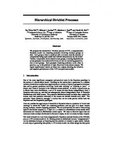
Fig. 7.1 The four acoustic common ways used to divide into units [3]. (a) Separated by silence. (b) Change in acoustic properties (regardless of silence). (c) Series of sounds. (d) Higher levels of organisation

interpret the identified song units in time. There is a lack of methodologies focused on real world data, and with further applications in ecology and wildlife management. One of the major bottlenecks for the application of these methodologies is their inability to work under heavy complex acoustic environment, where different taxa may sing together or conversely, their extreme sensitivity which may result in an over classification due to the high degree of variability insight many repertoire of the vocal species. In this paper, we model the sequence of a non-human signals and determine their acoustic song units. The way according to which non-human acoustic sequences can be interpreted can be summarized as shown in Fig. 7.1. Four common properties are used to define potential criteria for segmenting such signals into song units. The first way, shown in Fig. 7.1a, consists in separating the signals using silent gaps. The second way, shown in Fig. 7.1b, consists in separating the signals according to the changes in the acoustic properties in the signal. The third way, shown in Fig. 7.1c consists in grouping similar sounds separated with silent gaps as a single unit. The last common way, shown in Fig. 7.1d consists in separating signal in organized sound structure, considered as fundamental units. Manual segmentation is time consuming and not possible for a large acoustic dataset. That is why automatic approaches are needed. Furthermore, in bioacoustic signals, the problem of segmenting signals of many species, is still an issue. Hence, a well-principled learning system based on unsupervised approach can help to have a better understanding of bioacoustics species. In this context, we investigate statistical latent data models to automatically identify song units. First, we study Hidden Markov Models (HMMs) [4].The main issue with HMMs is to select the number of hidden states. Because of the lack of knowledge on non-human species, it is hard to have this number. This rises a model selection problem, which can be addressed by information selection criteria such as BIC, AIC [5, 6], which select an

7 Unsupervised Bioacoustic Segmentation. . .

115

HMM with a number of states from pre-estimated HMMs with varying number of states. Such approaches require learning multiple HMMs. On the other hand, nonparametric derivations of HMMs constitute a well-principled alternative to address this issue. Thus we used Bayesian parametric (BNP) formulation for HMMs [7], also called the infinite HMM (iHMM) [8]. It allows to infer the number of states (segments, units) from the data. The BNP approach for HMMs relies on Hierarchical Dirichlet Process (HDP) to define a prior over the states [7]. It is known as the Hierarchical Dirichlet Process for the Hidden Markov Models (HDP-HMM) [7]. The HDP-HMM parameters can be estimated by MCMC sampling techniques such as Gibbs sampling. The standard HDP-HMM Gibbs sampling has the limitation of an inadequate modeling of the temporal persistence of states [9]. This problem has been addressed by Fox et al. [9] by relying on a sticky extension which allows a more robust learning. Hence, we have a model to separate non-human signals into states that represent different activities (song units) and exploring the inference of complex data such as bioacoustic data in an environmental case (multispecies/multisources) this problem is not yet resolved. In this paper, we investigate the BNP formulation of HMM, that is the HDPHMM, into two challenges involving real bioacoustic data. First, a challenging problem of humpback whale song decomposition is investigated. The objective is the unsupervised structuration of whale bioacoustic data. Humpback whale songs are long cyclical sequences produced by males during the reproduction season which follows their migration from high-latitude to low-latitude waters. Singers from the same geographical region share parts of the same song. This leads to the idea of dialect [10]. Different hypotheses of these songs were emitted [11–14]. Next, we investigate a challenging problem of bird song unit structuration. Catchpole and Slater [15], Kroodsma and Miller [16] show how birds sing and why birds have such elaborate songs. However, analysing bird song units is difficult due to the transientness of typical bird chirps, the large behavioural intra-class variability, the small amount of examples per class, the presence of wildlife noise, and so forth. As shown later in the obtained segmentation results, such automatic approaches allow large-scale analysis of environmental bioacoustics recordings

7.1.1 Related Work Discovering the call units (which can be considered as a kind of non-human alphabet) of such complex signals can be seen as a problem of unsupervised call units classification as [1, 17]. Picot et al. [18] also tried to analyse bioacoustic songs using a clustering approach. They implemented a segmentation algorithm based on Payne’s principle to extract sound units from a bioacoustic song. Contrary to [17], in which the number of states (call units in this case) has been fixed by Davies Bouldin criteria, or [18] where a K-means algorithm is used, our approach is based on a probabilist

116

V. Roger et al.

approach on the MFCC1 ; it is non-parametric that is well-suited to the problem of automatically inferring the number of the states corresponding to the data. In the next section we describe the real-world bioacoustic challenges we used and explain our approach.

7.2 Data and Methods The data used represent the difficulties of bioacoustic problems, especially when the only information linked to the signal is the species name. Thus, we have to determine a sequence without ground truth.

7.2.1 Humpback Whale Data Humpback whale song data consist of a recording (about 8.6 minutes) produced at few meters from the whale in La Reunion—Indian Ocean [19],2 at a frequency sample of 44.1 kHz, 32 bits, one channel. We extract MFCC features from the signal, with pre-emphasis: 0.95, hamming window, FFT on 1024 points (nearly 23 ms), frameshift 10 ms, 24 Mel channels, 12 MFCC coefficients plus energy and their delta and acceleration, for a total of 39 dimensions as detailed in the NIPS 2013 challenge [19] where the signal and the features are available. The retained data for our experiment are the 51,336 first observations.

7.2.2 Multi-Species Bird Data Bird species song data from Fernand Deroussen Jerome Sueur of Musee National d’Histoire Naturelle [20], consists of a training and a testing set (not used here because it contains multiple species singing simultaneously). Theses sets were designed for the ICML4B challenge.3 The recordings have a frequency sample of 44.1 kHz, 16 bits, one channel. The training set is composed of 35 recordings, 30 s each taken from 1 microphone. Each record contains 1 bird species in the foreground for a total of 35 different birds species.

1 The

MFCC are features that represent and compress short-term power spectrum of a sound. It follows the Mel scale. 2 http://sabiod.univ-tln.fr/nips4b/challenge2.html. 3 http://sabiod.univ-tln.fr/icml2013/BIRD_SAMPLES/.


117

The feature extraction for this application is applied as follows. First, a high pass filter is processed to reduce the noise (set at 1.000 kHz to avoid noises). Then, we extract the MFCC features with windows of 0.06 s and shift of 0.03 s, we keep 13 coefficients, with energy as first parameter, to be compact and sufficient accurate, considering only the vocal track information and removing the source information. Also, we focus on frequencies below 8.000 kHz, because of the alterations into the spectrum. We obtain 34,965 observations with 13 dimensions each for train set, that is used to learn our model.

7.2.3 Method: Unsupervised Learning for Signal Representation To solve bioacoustic problems and finding the number of call units we propose to use the HDP-HMM model to model complex bioacoustic data. Our approach automatically discovers and infers the number of states from the non-human song data. In this paper we present two applications on bioacoustic data. We study the song unit structuration, for the humpback whale and for the multi-species birds signal. In the next section we give a brief description of the Hidden Markov Model and it’s Bayesian non-parametric used in our bioacoustic signal representation applications.

7.3 Bayesian Non-parametric Alternative for Hidden Markov Model The finite Hidden Markov Model (HMM) is very popular due to its stability to model sequential data (e.g. acoustic data). It assumes that the observed sequence X = (x1 , . . . , xT ) is governed by a hidden state sequence z = (z1 , . . . , zT ), where xt ∈ Rd is the multidimensional observation at time t and zt represents the hidden state of xt values in a finite set {1, . . . , K}, K being the number of states, that is unknown. The generative process of the HMM can be described in general by the following steps. First, z1 follows the initial distribution π1 . Then, given the previous state (zt−1 ), the current state zt follows the transition distribution. Finally, given the state zt , the observation xt follows the emission distribution F (θ zt ) of that state. The HMM parameters, that are the initial state transition (π1 ), the transition matrix (π), and the emission parameters (θ ) are in general estimated in a maximum likelihood estimation (MLE) framework by using the Expectation-Maximization (EM) algorithm, also known as the Bauch-Welch algorithm [21] in the context of HMMs.

118

V. Roger et al.

Therefore, for the finite HMM, the number of states K is required to be known a priori. This model selection issue can be addressed in a two-stage scheme by using model selection criteria such as the Bayesian Information Criterion (BIC) [5], the Akaike Information Criterion (AIC) [6], the Integrated Classification Likelihood criterion (ICL) [22], etc to select a model from pre-estimated HMMs with varying number of states. Such approaches are limited to learn N HMMs, N being sufficiently high to have an equivalent of a non parametric approach. In the light of this, a non parametric approach is more efficient because it theoretically tends to an infinite number of states. Thus, we use a Bayesian non-parametric (BNP) version of the HMM, that is able to infer the number of hidden states from the data. It is more flexible than learning multiple HMMs, because in bio-acoustic problems the model have to characterize multiple species/individuals, thus it possibly tends to a large number of hidden states. The BNP approach for the HMM, that is the infinite HMM (iHMM), is based on a Dirichlet Process (DP) [23]. However, as the transitions of states have independent priors, there is no coupling across transitions between different states [8], therefore the DP is not sufficient to extend the HMM to an infinite model. The Hierarchical Dirichlet Process (HDP) prior distribution on the transition matrices over countability infinite state space, derived by Teh et al. [7], extends the HMM to the infinite state space model and is briefly described in the next subsection.

7.3.1 Hierarchical Dirichlet Process (HDP) Suppose the data divided into J groups, each produced by a related, yet distinct process. The HDP extends the DP by an hierarchical Bayesian approach such that a global Dirichlet Process prior DP(α0 , G0 ) is drawn from a global prior Gj , where G0 is itself a Dirichlet Process distribution with two parameters, a base distribution H and a concentration parameter γ . The generative process of the data with the HDP can be summarized as follows. Suppose data X, with i = 1, . . . , T observations grouped into j = 1, . . . , J groups. The observations of the group j are given by Xj = (xj 1 , xj 2 , . . .), all observations of group j being exchangeable. Assume each observation is drawn from a mixture model, thus each observations xj i is associated with a mixture component, with parameter θj i . Note that from the DP property, we observe equal values in the components θj i . Now, giving the model parameter θj i , the data xj i is drawn from the distribution F (θj i ). Assuming a prior distribution Gj over the model parameters associated for group j , θ j = (θj 1 , θj 2 , . . .), we can define the generative process in Eq. (7.1). G0 |γ , H Gj |α0 , G0 θj i |Gj xj i |θj i

∼ ∼ ∼ ∼

DP(γ , H ), DP(α0 , G0 ), ∀j ∈ 1, . . . , J , Gj , ∀j ∈ 1, . . . , J and ∀i ∈ 1, . . . , T , F (xj i |θj i ), ∀j ∈ 1, . . . , J and ∀i ∈ 1, . . . , T .

(7.1)


119

The Chinese Restaurant Process (CRP) [24] is a representation of the Dirichlet Process that results from a metaphor related to the existence of a restaurant with possible infinite tables (clusters) where customers (observations) are sitting in it. An alternative of such a representation for the Hierarchical Dirichlet Process can be described by the Chinese Restaurant Franchise (CRF) process by extending the CRP to multiple restaurants that share a set of dishes. The idea of CRF is that it gives a representation for the HDP by extending a set of (J) restaurants, rather than a single restaurant. Suppose a patron of chinese restaurant creates many restaurants, strongly linked to each other, by a franchise wide menu, having dishes common to all restaurants. As a result, restaurants are created (groups) with a possibility to extend each restaurant with an infinite number of tables (states) at witch the customers (observations) sit. Each customer goes to his specified restaurant j , where each table of this restaurant has a dish between the customers that sit at that specific table. However, multiple tables of different existing restaurants can serve the same dish.

7.3.2 The Hierarchical Dirichlet Process for the Hidden Markov Model (HDP-HMM) The HDP-HMM uses a HDP prior distribution providing a potential countability infinite number of hidden states and tackles the challenging problem of model selection for the HMM. This model is a Bayesian non-parametric extension for the HMM also presented as the infinite HMM. To derive the HDP-HMM model we suppose a doubly-infinite transition matrix, where each row corresponds to a CRP. Thus, in a HDP formalism, the groups correspond to states, with CRP distribution on next states. CRF links these states distributions. We assume for simplicity a distinguished initial state z0 . Let Gj describes both, the transition matrix π k and the emission parameters θ k , the infinite HMM can be described by the following generative process: β|γ ∼ GEM(γ ),

π k |α, β ∼ DP(α, β),

zt |zt−1 ∼ Mult(π zt−1 ),

(7.2)

θ k |H ∼ H,

xt |zt , {θ k }∞ k=1 ∼ F (θ zt ). where, β is a hyperparameter for the DP [2] distributed according to the stick-breaking construction noted GEM(.); zt is the indicator variable of the HDP-HMM that follows a multinomial distribution Mult(.);

120

V. Roger et al.

the emission parameters θ k , are drawn independently, according to a conjugate prior distribution H ; F (θ zt ) is a data likelihood density with the unique parameter space of θ zt equal to θk. Suppose the observed data likelihood is a Gaussian density N (xt ; θ k ) where the emission parameters θ k = {µk , Σ k } are respectively the mean vector µk and the covariance matrix Σ k . According to [25], the prior over the mean vector and the covariance matrix is a conjugate Normal-Inverse-Wishart distribution, denoted as N I W (µ0 , κ0 , ν0 , Λ0 ), with the hyper-parameters describing the shapes and the position for each mixture components: µ0 is the mean of Gaussian should be, κ0 the number of pseudo-observations supposed to be attributed, and ν0 , Λ0 being similarly for the covariance matrix. In the generative process given in Eq. (7.2), π is interpreted as a double-infinite transition matrix with each row taking a CRP. Thus, in the HDP formulation the group-specific distribution, π k corresponds to the state-specific transition where the CRF defines distributions over the next state. In turn, [9] showed that HDPHMM inadequately models the temporal persistence of states, creating redundant and rapidly switching states and proposed an additional hyperparameter κ that increase the self-transition probabilities. This is named as sticky HDP-HMM. The distribution on the transition matrix of Eq. (7.2) for the sticky HDP-HMM is given as follows: " ! αβ + κδk π k |α, β ∼ DP α + κ, , (7.3) α+κ where a small positive κ > 0 is added to the k th component of αβ, thus of selftransition probability is increased by κ. Note that setting κ to 0, the original HDPHMM is recovered. Under such assumption for the transition matrix, [9] proposes an extension of the CRF to the Chinese Restaurant Franchise with Loyal Customers. A graphical representation of (sticky) HDP-HMM is given in Fig. 7.2. Fig. 7.2 Graphical representation of sticky Hierarchical Dirichlet Process for Hidden Markov Model (HDP-HMM)


121

The inference of the infinite HMM (the (sticky) HDP-HMM) with the Block Gibbs sampler algorithm is given in Algorithm 3 of Supplementary Material in [9] paper. The basic idea of this sampler is to estimate the posterior distributions over all the parameters from the generative process of (sticky) HDP-HMM given in Eq. (7.2). Here, the CRF with loyal customers, hyperparameter κ of the transition matrix can be sampled in order to increase the self-transition probability. Hence, the HDP-HMM model resolves the problem of advanced signal decomposition using acoustic features with respect to time. It allows identifying song units (states), behaviour and enhancing populations studies. From the other point, modelling data with the HDP-HMM offers a great alternative of the standard HMM to tackle the challenging problem of selecting the number of states, identifying the unknown number of hidden units from the used features (here: MFCC). The experimental results show the interest of such an approach.

7.4 Experiments In this section we present two applications on bioacoustic data. We study the song unit structuration, for the humpback whale signal and for multi-species birds signals.

7.4.1 Humpback Whale Sound Segmentation The learning of the humpback whale song, applied via the HDP-HMM, is done with the Blocked Gibbs sampling. A number of iterations was fixed to Ns = 30,000 and a truncation level, that corresponds to the maximum number of possible states in the model (being sufficient big to approximate it to an infinite model), is fixed to Lk = 30. The number of states estimated by the HDP-HMM Gibbs sampling is six. Figure 7.3 shows the state sequences partition, for all 8.6 min of humpback whale song data, obtained by the HDP-HMM Gibbs sampling. For more detailed information, the result of the whole humpback whale signal segmentation is separated by several parts of 15 s. All the spectrograms of the humpback whale song and the obtained segmentation are made available in the demo: http://sabiod. univ-tln.fr/workspace/MTAP/whale.zip. This demo highlights the interest of using a BNP formulation of HMMs for unsupervised segmentation of whale signals. Three examples of the humpback whale song, with 15 s duration each, are presented and discussed in this paper (see Fig. 7.5). Figure 7.5 represents the spectrogram and the corresponding state sequence partition obtained by the HDP-HMM Gibbs inference algorithm. They respectively represent examples of the beginning, the middle and the end of the whole signal.

122

V. Roger et al.

1

Song units

2

3

4

5

6 Total time (8.6min)

Fig. 7.3 State sequence for 8.6 min of humpback whale song obtained by the Blocked Gibbs sampling inference approach for HDP-HMM 8000 7000 Frequency in Hz

Frequency in Hz

8000 6000 4000

6000 5000 4000 3000 2000

2000

1000 0 0

5

10

15

Time in seconds

20

25

0

2

4

6

8

10

Time in seconds

Fig. 7.4 Spectrograms of the 6th whale song unit (left) and 2nd song unit (right)

All the obtained state sequence partitions fit the spectral patterns. We note that the estimated state 1 fits the sea noise, state 5 also fits sea noise, but it is right before units associated to whale songs. The presence of this unit can be due to an insufficient number of Gibbs samples. For a longer learning the fifth state could be merged with the first state. State 2 fits the up and down sweeps. State 3 fits low and high fundamental harmonic sounds, state 4 fits for numerous harmonics sound and state 6 fits very noisy and broad sounds. Figure 7.4 shows two spectrograms extracted from the 6th song unit (left) and from the 2nd song unit (right) of the whole humpback whale signal. We can see that the units fit specific patterns on the whole signal. Pr. Gianni Pavan (Pavia University, Italy), undersea NATO bioacoustic expert analysed the results on these humpback whale song segmentations we produced

123

Freq [0,5500] Hz


Song units

1 2 3 4 5 6 4

6 8 10 Time in seconds

12

14

2

4


12

14

2

4


12

14

Freq [0,5500] Hz

2

Song units

1 2 3 4 5

Freq [0,5500] Hz

6

Song units

1 2 3 4 5 6

Fig. 7.5 Obtained song units starting at 60 s (left), 255 s (middle) and 495 s (right). The spectrogram of the whale song (top), and the obtained state sequence (bottom) by the Blocked Gibbs sampler inference approach for the HDP-HMM. The silence (unit 1 and 5) looks well separated from the whale signal. Whale up and down sweeps (unit 2), harmonics (unit 3 and 4) and broad sounds (unit 6) are also present

124

V. Roger et al.

in this paper. He validated the computed representation, as the usual optimal segmentation an expert produces. This highlight the interest of learning BNP model on a single species to produce expert representation. In the next section we validate the approach on several bird species.

7.4.2 Birds Sound Segmentation In this section we describe the obtained bird song unit segmentation. We segment the bird signals into song units by learning the HDP-HMM model on the training set (containing 35 different species). The main goal is to see if a such approach can model multiple species. Note that in this set, we assume there is no multiple species singing at the same time. For this application, we considered 14,5000 Gibbs iterations and a truncation level of 200 for the maximum number of states. We suppose them to be sufficiently big for this data problem. Moreover, we use one mixture component per state, that appeared to give satisfactory results and we use a sticky HDP-HMM with the hyperparameter κ set to 0.1. We discovered 76 song units with this method. For more detailed information over the signal, we separated the whole train set into parts of 15 s each. All the spectrograms and the associated segmentation obtained are made available in the demo: http://sabiod.univ-tln.fr/workspace/MTAP/bird.zip. 7.4.2.1

Evaluation of the Bird Result

To evaluate the bird results, we used a ground truth produced by an expert ornithologist. He segmented each recording of the dataset according to the different patterns on the signal. Then we compare this ground truth with the segments produced by the model using the Normalized Mutual Information NMI [26] which calculates shared information between two clustering sets. We computed the NMI score for each species, as reported in Table 7.1. The highest score is 0.680 (Corvus Corone) and the lowest score is 0.003 (Garrulus Glandarius). Thus, for some species, the model has difficulties to segment the data. Sometimes, it uses less states than the expert to segment the data: for the Oriolus Oriolus (Golden Oriole), the model identifies 12 song units versus 50 identified by the expert. Nevertheless, the model also uses more states than the expert to segment the data: for the Fringilla Coelebs (chaffinch), the model identifies 15 song units versus 3 identified by the expert. In other cases, the model can’t differentiate 2 distinct vocalizes if they have close frequencies (Phylloscopus Collybita and Columba Palumbus), background and foreground species (Streptopelia Decaocto). This can be due to the feature used (wrong time scale), or to an insufficient number of iterations of the Gibbs sampling. For most of species, the model and the ground truth have similar patterns observable on Figs. 7.6, 7.8 and 7.7, but not in the sample Figs. 7.10 and 7.9.

7 Unsupervised Bioacoustic Segmentation. . . Table 7.1 NMI score for the obtained segmentation using HDP-HMM

125 Species Corvus corone Picus viridis Fringilla coelebs Emberiza citrinella Parus palustris Luscinia megarhynchos Dendrocopos major Prunella modularis Sturnus vulgaris Pavo cristatus Certhia brachydactyla Turdus viscivorus Parus caeruleus Troglodytes troglodytes Sylvia atricapilla Turdus philomelos Turdus merula Erithacus rubecula Carduelis chloris Columba palumbus Branta canadensis Anthus trivialis Sitta europaea Oriolus oriolus Streptopelia decaocto Phoenicurus phoenicurus Phasianus colchicus Parus major Phylloscopus collybita Cuculus canorus Aegithalos caudatus Strix aluco Alauda arvensis Motacilla alba Garrulus glandarius Mean

NMI score 0.680 0.602 0.565 0.534 0.521 0.497 0.481 0.476 0.467 0.437 0.417 0.417 0.413 0.407 0.405 0.398 0.395 0.394 0.385 0.352 0.339 0.332 0.332 0.316 0.306 0.291 0.272 0.270 0.267 0.205 0.202 0.200 0.169 0.105 0.003 0.367

126

V. Roger et al.

Fig. 7.6 Picus viridis with a high NMI score of 0.602. Top: the labelled ground truth over 30 s where label 0 is always the silence label and the other labels are specific to each species. Medium: our model with the 76 classes. Bottom: spectrogram

Fig. 7.7 Corvus corone, high NMI score of 0.68 (cf. Fig. 7.6)


Fig. 7.8 Fringilla coelebs, medium NMI score 0.565 (cf. Fig. 7.6)

Fig. 7.9 Motacilla alba, low NMI score 0.105 (cf. Fig. 7.6)

127

128

V. Roger et al.

Fig. 7.10 Garrulus glandarius, low NMI score 0.003 (cf. Fig. 7.6)

To improve the model, we can investigate better feature representation for species with different acoustic characteristics. We can also improve noise reduction which could be useful for background activities. Also, it can be dur to the fact we use one annotator. Nevertheless, the application highlights the interest of using BNP formulation of HMMs for unsupervised segmentation of bird signals.

7.5 Conclusions We proposed BNP HMM formulation to a representation of real world bioacoustic scenes. The evaluations on two challenges, available online, show the efficiency of the method, which forms a possible answer to the questions opened in [3]. The BNP formulation gives an estimate number of cluster needed to segment the signal and our experiments highlight the interest of such formulation on bioacoustic problems. We score with NMI the segmentation obtained for birds with the segmentation from an expert, showing promising results.One of the main topic in ecological acoustics is the development of unsupervised methods for automatic detection of vocalized species, which would help specialists in ecological works during their monitoring activities.Future work will consist in the MCMC sampling dealing with larger data


129

problems, like variational inference [27] or stochastic variational inference used for HMMs [28], joint to feature learning to automatically adapt time frequency scales to each species. Acknowledgements We would like to thanks Provence-Alpes-Côte d’Azur region and NortekMed for their financial support for Vincent ROGER. We also thank GDR CNRS MADICS http://sabiod.org/EADM for its support. We thank G. Pavan for its expertise, J. Sueur, F. Deroussen, F. Jiguet for the coorganisation of the challenges and M. Roch for her collaboration.

References 1. Bartcus, M., Chamroukhi, F., & Glotin, H. (2015, July). Hierarchical Dirichlet Process Hidden Markov Model for Unsupervised Bioacoustic Analysis. In Neural Networks (IJCNN), 2015 International Joint Conference on pp. 1–7. IEEE. 2. Sethuraman, J. (1994). A constructive definition of Dirichlet priors. Statistica sinica, 639–650. 3. Kershenbaum, A., Blumstein, D.T., Roch, M.A., Akçay, Ç., Backus, G., Bee, M.A., Bohn, K., Cao, Y., Carter, G., Cäsar, C. and Coen, M. (2016). Acoustic sequences in non-human animals: a tutorial review and prospectus. Biological Reviews, 91(1), pp.13–52. 4. Rabiner, L. and Juang, B. (1986). An introduction to hidden Markov models. ieee assp magazine, 3(1), pp.4–16. 5. Schwarz, G. (1978). Estimating the dimension of a model. The annals of statistics, 6(2), pp.461–464. 6. Akaike, H. (1974). A new look at the statistical model identification. IEEE transactions on automatic control, 19(6), 716–723. 7. Teh, Yee Whye and Jordan, Michael I. and Beal, Matthew J. and Blei, David M. (2006). Hierarchical Dirichlet Processes. Journal of the American Statistical Association, 476(101), pp.1566–1581. 8. Beal, M. J., Ghahramani, Z., & Rasmussen, C. E. (2002). The infinite hidden Markov model. In Advances in neural information processing systems pp. 577–584. 9. Fox, E. B., Sudderth, E. B., Jordan, M. I., & Willsky, A. S. (2008, July). An HDP-HMM for systems with state persistence. In Proceedings of the 25th international conference on Machine learning pp. 312–319. ACM. 10. Helweg, D.A., Cat, D.H., Jenkins, P.F., Garrigue, C. and McCauley, R.D. (1998). Geograpmc Variation in South Pacific Humpback Whale Songs. Behaviour, 135(1), pp.1–27. 11. Medrano, L., Salinas, M., Salas, I., Guevara, P.L.D., Aguayo, A., Jacobsen, J. and Baker, C.S. (1994). Sex identification of humpback whales, Megaptera novaeangliae, on the wintering grounds of the Mexican Pacific Ocean. Canadian journal of zoology, 72(10), pp.1771–1774. 12. Frankel, A.S., Clark, C.W., Herman, L. and Gabriele, C.M. (1995). Spatial distribution, habitat utilization, and social interactions of humpback whales, Megaptera novaeangliae, off Hawai’i, determined using acoustic and visual techniques. Canadian Journal of Zoology, 73(6), pp.1134–1146. 13. Baker, C.S. and Herman, L.M. (1984). Aggressive behavior between humpback whales (Megaptera novaeangliae) wintering in Hawaiian waters. Canadian journal of zoology, 62(10), pp.1922–1937. 14. Garland, E.C., Goldizen, A.W., Rekdahl, M.L., Constantine, R., Garrigue, C., Hauser, N.D., Poole, M.M., Robbins, J. and Noad, M.J. (2011). Dynamic horizontal cultural transmission of humpback whale song at the ocean basin scale. Current Biology, 21(8), pp.687–691. 15. Catchpole, C.K. and Slater, P.J., 86. B. (1995). Birdsong: Biological Themes and Variations. Cambridge University PressCatchpole.

130

V. Roger et al.

16. Kroodsma, D. E., & Miller, E. H. (Eds.). (1996). Ecology and evolution of acoustic communication in birds pp. 269–281. Comstock Pub. 17. Pace, F., Benard, F., Glotin, H., Adam, O. and White, P. (2010). Subunit definition and analysis for humpback whale call classification. Applied Acoustics, 71(11), pp.1107–1112. 18. Picot, G., Adam, O., Bergounioux, M., Glotin, H. and Mayer, F.X. (2008, October). Automatic prosodic clustering of humpback whales song. In New Trends for Environmental Monitoring Using Passive Systems, 2008 pp. 1–6. IEEE. 19. Glotin, H., LeCun, Y., Artieres, T., Mallat, S., Tchernichovski, O., & Halkias, X. (2013). Neural information processing scaled for bioacoustics, from neurons to big data. USA (2013). http:// sabiod.org/NIPS4B2013_book.pdf. 20. Deroussen F., Jiguet F. (2006). La sonotheque du Museum: Oiseaux de France. Nashvert Production, Charenton, France. 21. Baum, L.E., Petrie, T., Soules, G. and Weiss, N. (1970). A maximization technique occurring in the statistical analysis of probabilistic functions of Markov chains. The annals of mathematical statistics, 41(1), pp.164–171. 22. Biernacki, C., Celeux, G. and Govaert, G. (2000). Assessing a mixture model for clustering with the integrated completed likelihood. IEEE transactions on pattern analysis and machine intelligence, 22(7), pp.719–725. 23. Ferguson, T.S. (1973). A Bayesian analysis of some nonparametric problems. The annals of statistics, pp.209–230. 24. Pitman, J. (1995). Exchangeable and partially exchangeable random partitions. Probability theory and related fields, 102(2), pp.145–158. 25. Gelman, A., Carlin, J. B., Stern, H. S., & Rubin, D. B. (2003). Bayesian Data Analysis, (Chapman & Hall/CRC Texts in Statistical Science). 26. Strehl, A. and Ghosh, J. (2002). Cluster ensembles—a knowledge reuse framework for combining multiple partitions. Journal of machine learning research, 3(Dec), pp.583–617. 27. Jordan, M.I., Ghahramani, Z., Jaakkola, T.S. and Saul, L.K. (1999). An introduction to variational methods for graphical models. Machine learning, 37(2), pp.183–233. 28. Foti, N., Xu, J., Laird, D., & Fox, E. (2014). Stochastic variational inference for hidden Markov models. In Advances in neural information processing systems, pp.3599–3607.