Current software quality estimation models often in- volve using supervised learning methods to train a soft- ware quality classifier or a software fault prediction.
Unsupervised Learning for Expert-Based Software Quality Estimation Shi Zhong, Taghi M. Khoshgoftaar, and Naeem Seliya Department of Computer Science and Engineering Florida Atlantic University, Boca Raton, FL 33431, USA {zhong,taghi,nseliya}@cse.fau.edu Abstract Current software quality estimation models often involve using supervised learning methods to train a software quality classifier or a software fault prediction model. In such models, the dependent variable is a software quality measurement indicating the quality of a software module by either a risk-based class membership (e.g., whether it is fault-prone or not fault-prone) or the number of faults. In reality, such a measurement may be inaccurate, or even unavailable. In such situations, this paper advocates the use of unsupervised learning (i.e., clustering) techniques to build a software quality estimation system, with the help of a software engineering human expert. The system first clusters hundreds of software modules into a small number of coherent groups and presents the representative of each group to a software quality expert, who labels each cluster as either fault-prone or not fault-prone based on his domain knowledge as well as some data statistics (without any knowledge of the dependent variable, i.e., the software quality measurement). Our preliminary empirical results show promising potentials of this methodology in both predicting software quality and detecting potential noise in a software measurement and quality dataset.
1
Introduction
Estimating the quality of a software product during its development or pre-operation phases is a challenging problem, especially when there is very limited or no information regarding its existing quality is available. In software quality estimation problems, a software quality classification [10, 15] or software fault prediction model [9] is typically trained or built using software measurements and fault data from a previous system release or similar software project developed by the given organization. These models are supervised learn-
ing in the sense that the training process is guided by the software quality measurement (i.e., the dependent variable or the fault-proneness label1 ). The trained model is then used to predict the quality of the software modules in a software project under consideration. In this paper, we are particularly interested in learning software quality estimation models using unsupervised learning methods in the absence of software quality measurements. In a high-assurance software system, such as telecommunications and medical systems, the assurance of software quality and reliability is a critical component of the software development process. The management of such systems is often interested in constantly tracking and estimating the quality of the software. However, the software quality measurement knowledge may not be available for training a software quality estimation model. Such a software engineering situation may occur when the organization is dealing with a software project type for which it does not have a similar experience in the past. In addition, the software quality measurements in a previous system release may not have been collected and recorded. Hence the question is: how does the software quality assurance team predict the software quality (of the project under development) based on only the recorded software metrics? Under such situations, a supervised learning approach cannot be taken for software quality estimation due to the absence of software quality measurements. The estimation task then falls on the analyst who has to decide the fault-proneness for each software module. Unsupervised learning methods, such as clustering techniques, are more appropriate for building the models in the absence of software quality data. Clustering algorithms can group the software modules according 1 To make this paper accessible to readers from different disciplines (e.g., software engineering and machine learning), we interchangeably use dependent variable, software quality measurement, fault-proneness label, and risk-based class to refer to the same concept.
to the values of their software metrics. The underlying software engineering assumption is that the faultprone software modules will have similar software measurements, and hence are likely to be grouped together in the same cluster(s). Similarly, the not fault-prone modules will likely be grouped in the same cluster(s). In this paper, we study two clustering techniques—kmeans [13] and Neural-Gas [14]—for grouping the unlabeled (not classified as per fault-proneness) modules of a high-assurance software system. Upon the completion of clustering analysis, the software engineering expert inspects different clusters and labels them as either fault-prone or not fault-prone. A clustering approach for grouping the software modules is of practical benefit to the expert who has to decide the labels of individual software modules. Instead of inspecting and labeling each module one at a time, an expert can inspect and label a given cluster as a whole, i.e., all the modules in the cluster will be assigned the same quality label. Such a strategy leverages upon clustering techniques to group similar modules together as coherent clusters, and eases the tedious (compounded when the number of modules is very large) labeling problem for the expert. In the case of each cluster, the clustering algorithm can provide a representative software module, which can be inspected by the expert for labeling all the modules in that cluster (with the help of other data statistics, see Section 5.1). Moreover, when the fault-proneness labels are available (either based on software faults discovered during postrelease or heuristic information), they can be used to evaluate the effectiveness of the clustering- and expertbased approach and provide valuable feedback to the expert for improving the labeling of software modules in future releases of a given software project or those of other software projects. The main contribution of this paper is a clusteringand expert-based methodology for estimating software quality in practical software engineering systems in the absence of software quality measurements. The clustering approach to software quality estimation presented in this paper is also attractive for addressing the noise detection and removal problem for software quality classification. More specifically, for a given cluster if a big majority of software modules are not fault-prone and a few modules are fault-prone, then an educated assessment can be that the few fault-prone modules in the cluster are likely noise. Our future work shall investigate more on the clustering-based noise detection issue for software quality estimation. This paper is organized as follows. Section 2 briefly discusses related research work. Section 3 describes the two clustering algorithms studied in this paper. Sec-
tion 4 presents our clustering- and expert-based software quality estimation methodology. Section 5 explains the setup of our experimental study and discusses the results. Finally, concluding remarks are given in Section 6.
2
Related Work
In the context of software quality estimation, most research works have focused on using supervised learning methods for building software quality classification or software fault prediction models. To our knowledge, there has been almost no or very little effort devoted to unsupervised learning for software quality estimation. Fuzzy clustering was used by Yuan et al. [19] to predict the number of faults in software modules. The specific “clustering” algorithm used in their paper, however, is actually a regression model with the dependent variable involved in the training. An unsupervised analysis of software measurement data using self-organizing maps is provided in [16]. In their study, the authors primarily used the twodimensional visualization capabilities of self-organizing maps for analyzing the similarity of the modules according to their software metrics. They present an indepth discussion of which software measures are important for a given group of software modules. However, in contrast to our study, their work does not focus on the software quality estimation problem. An unsupervised approach for extracting principal components from software measurement data using artificial neural networks is provided in [12]. The unsupervised training aspect of their study focuses only on extracting the principal components from software measurement data. The extracted components are then used to train a supervised neural network-based software quality classification model for predicting the quality of software modules as fault-prone or not faultprone.
3
Clustering Techniques
Generally speaking, clustering techniques can be divided into pairwise clustering and central clustering. The former, also called similarity-based clustering, groups similar data instances together based on a data-pairwise proximity measure. Examples of this category include graph partitioning type methods [8]. The latter, also called centroid-based or model-based clustering, represents each cluster by a model, i.e., its “centroid”. For the well-known k-means algorithm, the “centroid” of a cluster is just the mean vector of the
cluster. Each data point is assigned to one or more clusters based on its distance to different cluster “centroids”. Centroid-based clustering algorithms are often more efficient than similarity-based clustering algorithms [20]. Regular k-means [13] and EM (Expectation Maximization) clustering [2, 4] belong to this category. We choose centroid-based approaches over similarity-based ones due to efficiency. Similarity-based algorithms usually have a complexity of at least O(N 2 ) (for computing the data-pairwise proximity measures), where N is the number of data instances. In contrast, centroidbased algorithms are more scalable, with a complexity of O(N KM ), where K is the number of clusters and M the number of batch iterations. A batch iteration means going through all training data points one round and, in contrast, an online iteration means after visiting one data point. The reason for selecting k-means is due to its popularity and efficiency whereas Neural-Gas is used for its good performance in producing coherent clusters [14].
Algorithm: k-means clustering Input: A set of N data vectors X = {x1 , ..., xN } in IRd and the number of clusters K. Output: A partition of the data vectors given by the cluster identity vector Y = {y1 , ...yN }, yn ∈ {1, ..., K} . Steps: 1. Initialization: Initialize the cluster centroid vectors {µ1 , ..., µK } ; 2. Data assignment: For each data vector xn , set yn = arg min kxn − µk k2 ; k
3. Centroid estimation: For cluster k, let Xk = {xn |yP n = k}, the centroid is estimated as µk = 1 x; |Xk | x∈X k
4. Stop if Y does not change, otherwise go back to Step 2.
Figure 1. Standard k-means clustering algorithm.
3.1 K-means The widely used standard k-means algorithm [13] is shown in Fig. 1. It can be seen as an optimization process that aims to minimize the following objective function (mean-squared error): M SE =
1 X kxn − µyn k2 , N n
(1)
where yn = arg mink kxn − µk k2 is the cluster identity of data vector xn and µyn the centroid of cluster yn . Unless specifiedpotherwise, k · k represents L2 P 2 norm. That is, kxk = d x(d) , where x(d) is the dth dimension of data vector x. Detailed settings on initialization and number of iterations (or convergence criterion) are provided in Section 5.2.
minima. In an annealing process, the temperature parameter is initially set high to equalize the probabilities of a data vector being assigned to different clusters; it is then gradually reduced over iterations to restrict a data vector to go to its closest “centroid” with a greater probability at each later iteration. Let x be a data vector, y the cluster index, and µy the centroid (mean) of cluster y. The batch version of the Neural-Gas algorithm amounts to iterating between the following two steps: e−r(x,y)/β , −r(x,y 0 )/β y0 e
P (y|x) = P and µy =
3.2 Neural-Gas (NGas) The Neural-Gas clustering algorithm [14] is a competitive learning technique with SoftMax 2 learning rule [1]. It is closely related to the Self-Organizing Map algorithm [11] and maximum entropy clustering [18]. A deterministic annealing mechanism [18] is built in the learning/optimization process to avoid many shallow 2 That is, multiple centroids get updated whenever a data instance is visited. The amount of update depends on the distance between the data instance and the cluster centroid. This is in contrast to the Winner-Take-All rule used in the k-means algorithm, where only one centroid gets updated every time an instance is visited.
1 X P (y|x)x , N x
(2)
(3)
where β is an equivalent temperature parameter that controls the smoothness of error surface, and r(x, y) is a rank function that takes the value k − 1 if y is the k th closest cluster centroid to data vector x. Therefore, there is a rank of clusters relative to each data instance x, and the assignment probability P (y|x) decreases as the rank of cluster y goes down. Both the k-means and Neural-Gas algorithms have online versions, in which the cluster centroids are updated incrementally when each data vector is visited. The online update rules can be found in [5, 14]. It has been shown that an online version of the Neural-Gas
algorithm can converge faster and find better local solutions than the Self-Organizing Map and maximum entropy clustering techniques [14].
4
Unsupervised Software Quality Estimation
The word “unsupervised” here refers to learning without class labels (i.e., the dependent variable) and not to learning without human supervision. We emphasize this to avoid confusion since our software quality estimation process involves a software engineering expert who “supervises” the labeling efforts. Our clustering- and expert-based software quality estimation is an interactive process. First, depending on the time availability of an expert, we determine a realistic range for number of clusters K. Such an approach is important for software projects where resources are relatively limited and finite. The mean (of software attribute values) of each cluster is then presented to the expert as the cluster representative. The expert also specifies other statistics from the software measurement dataset needed to accurately label each cluster as either fault-prone or not fault-prone. In our study, the provided data statistics include global mean, minimum, maximum, median, 75 percentile, and 90 percentile of each feature (software metric) dimension, as well as the size of each cluster. Of course, in the interactive process, the clustering analyst can suggest other useful information to the expert, who in turn may ask for additional data properties. We note that the cluster representatives are not immediately available for similarity-based clustering approaches, which further supports our choice of centroidbased clustering. In our study, the clustering analyst is a professional specializing in data mining and machine learning techniques, while the labeling expert is a professional with over fifteen years of experience in software quality and reliability engineering. The interactive process can be expedited if the clustering analyst and the software engineering expert are the same person; however, one has to be careful in staying away from introducing bias into the analysis.
5
Experimental Study
5.1 System Description The empirical case study presented is that of a NASA software project written in the C++ programming language. The software measurements and quality data was obtained through the NASA Metrics
Data Program (http://mdp.ivv.nasa.gov). The software metrics and fault data for the project was collected at the program’s function or subroutine levels. The data set has 520 software modules, each of which is characterized by thirteen software metrics. In this case study, a software module is a function, a subroutine, or a method. Table 1. Software Metrics. Branch Count metric
Line Count metrics
Halstead metrics
McCabe Metrics
Branch Count Total Lines of Code Executable LOC Comments LOC Blank LOC Code And Comments LOC Total Operators Total Operands Unique Operators Unique Operands Cyclomatic Complexity Essential Complexity Design Complexity
The thirteen software metrics used in our study are shown in Table 1. The collection and use of a given set of software metrics is dependent on the available metrics data collection tools and the software project under consideration. Another software project may consider a different set of software measurements for software quality estimation [3, 6, 17]. Some basic data statistics that are provided to the software engineering expert are shown in Table 2. They are derived based on interaction with the expert and used by the expert in his labeling effort. Each row in the table is one software metric, and the row-order in the table is the same as in the previous table, i.e., Table 1. The software modules are also characterized by two quality measurements: Error Rate—number of software faults in a module, and Defect—whether or not a module is fault-free. The latter is just a thresholdbased version of the former. A majority of the software modules have no faults. A total of 106 modules have one or more software faults, and the module with the largest number of faults has 13 faults. The remaining 414 software modules are fault free. A module with no defect is labeled as 0, i.e., not fault-prone, while those with one or more faults are labeled as 1, i.e., faultprone. In our clustering- and expert-based analysis, however, the labels of the modules are not used; They are only used for evaluating the expert’s decision of which clusters are fault-prone and which are not fault-
Table 2. Expert-specified data statistics. min 1 1 0 0 0 0 1 0 1 0 1 1 1
max 361 1275 1107 44 121 11 2469 1513 47 325 180 125 143
mean 8.79 37.03 27.87 2.0 4.35 0.28 57.83 37.16 9.23 14.52 4.91 2.45 3.66
median 3 13 8 0 1 0 17 11 8 7 2 1 2
75% 9 45 34 2 5 0 64 41 14 20 5 1 4
90% 19 91 71 5 11 1 142 95 18 37 10 5 7
prone.
5.2 Experimental Setting Both the k-means and Neural-Gas algorithms are implemented in C, with an interface to Matlab and compiled into mex files that can be called directly from Matlab. The executables are in binary code thus run faster than regular Matlab code. Batch training was used for the k-means algorithm with a relative convergence criterion of 1e-4 (i.e., if the relative change of cost function between two consecutive iterations is less than 1e-4 ). For the dataset we have, the k-means algorithm always converges within 100 iterations. We used an online version of the Neural-Gas algorithm and the temperature parameter β starts at K 2 and gradually decreases to 0.01 at the end of 100 batch iterations. We set the number of clusters K (a parameter needed by both the k-means and Neural-Gas algorithms) to 20. The heuristic consideration for choosing 20 is a balance between reducing the number of software module representatives examined by the expert and obtaining a fine (granularity) representation of the original software measurement data. Both the k-means and Neural-Gas algorithms generated a few empty clusters (4 and 2, respectively); thus the actual number of clusters evaluated by the expert is less than 20. Therefore, instead of evaluating 520 software modules one by one, the expert only needs to label less than 20 groups based on the respective cluster centroids, other data statistics, and his software engineering knowledge. For clustering quality, we use the mean squared error (mse) objective (Equation (1)) and average purity (ave-pur ). The purity of a cluster is defined as the percentage of the most dominated category (fault-prone or not fault-prone) in the cluster, and average purity is
the mean over all clusters. It has a range of between 0 and 1; the higher the number, the better is the average purity. To evaluate the expert’s labeling decision, we use the Defect labels that was provided with the dataset but not being used in the expert-based labeling process. Specifically, the overall classification error (error, percentage of mislabeled modules by the expert), false positive rate (fpr, percentage of not fault-prone modules labeled as fault-prone by the expert), and false negative rate (fnr, percentage of fault-prone modules labeled as not fault-prone) are reported.
5.3 Clustering and Quality Estimation Results The clustering quality results are shown in Table 3. The Neural-Gas algorithm performs significantly better in terms of mse and slightly better in terms of average purity. The k-means algorithm, however, runs much faster. The run time results are recorded on a 3.06GHz Pentium 4 PC running Windows XP. Table 3. Clustering Results. k-means NGas
mse 738.3 244.0
ave pur 0.808 0.815
time (seconds) 0.016 0.375
Table 4 reports the overall classification error, false positive rate, and false negative rate results, for both k-means and Neural-Gas algorithms. The Neural-Gas algorithm performs only slightly better even though in the previous table it gives significantly lower mse value. These numbers are very comparable to other classification-based approaches (e.g., a decision treebased classifier). One point worth mentioning here is that the dataset is difficult even for many state-of-theart classifiers. For example, we observe that the support vector machine method3 achieves only 20% overall classification error, with a false positive rate of 0 but a false negative rate of 98%. That is, the support vector machine method classifies almost all data as not faultprone. Therefore, the promising classification error results in Table 4 warrant more future investigations in building clustering- and expert-based software quality systems. A feedback from the expert shows that the NeuralGas results seem to be easier to label than the k-means results. It is not clear at this point, however, whether 3 The libsvm software package (available from http://www.csie.ntu.edu.tw/∼cjlin/libsvm/) was used with a two-fold cross validation setting.
Table 5. “Noise” vs. Mislabeled Modules.
Table 4. Evaluation of Expert’s Labeling. k-means NGas
error 18.27% 16.54%
fpr 14.98% 12.08%
mislabeled
fnr 31.13% 33.96%
this is accidental to our specific dataset. Future comparison on other datasets will be conducted.
k-means
95
Ngas
86
5.4 Noise Detection Results As noted above, the software engineering dataset for the case study is a very difficult one for classification analysis. Without a user-specified preferred balance between fpr and fnr, a classifier usually puts most data instances in the not fault-prone category. We thus suspect there is noise in the dataset, which can be those modules with very similar (or even identical) attribute values but having different Defect labels. In a recent study [7], we performed some preliminary work on detecting noise using multiple classifiers. The basic idea in that study was to use a set of different classifiers (as an ensemble-classifier filter) to classify the same dataset and predict the software modules that are misclassified by a given number of majority classifiers as potential noise. We used twenty-five different classifiers in the ensemble-classifier filter. In this section, we compare the “noise” modules identified by the ensemble classifier approach with those mislabeled by the expert in our clustering-based method. The results show an interesting match between the two sets of modules. Table 5 shows the matching results. The second column shows the number of mislabeled modules by the expert, the third column indicates the level of consensus4 among the 25 classifiers used for noise-filtering, the fourth column shows the number of “noise” software modules identified, and the last column indicates the recall percentage of the “noise” modules (i.e., how many modules identified as “noise” by the ensemble classifier approach are covered by the set of modules mislabeled by the expert). It is interesting to notice that a majority of the modules detected as “noise” are among the modules mislabeled by our clustering- and expert-based labeling method. Of course, currently we do not know which one (the ensemble classifier method or the clustering method) is more accurate for this case study. That leaves ample space for future research. 4 For example, 13C means that a module is viewed as “noise” if 13 or more classifiers (out of 25) predict the label wrong.
6
noise filter 25C 23C 17C 13C 25C 23C 17C 13C
“noise” modules 26 63 83 100 26 63 83 100
recall (%) 96.15 95.24 90.36 82 92.31 87.3 78.31 70
Conclusion
In this paper we have proposed a clustering- and expert-based software quality estimation method, targeting the practical software engineering situations when the Defect labels are inaccurate or unavailable. Promising experimental results have been shown through a study on a real dataset from a NASA software project, with two different clustering methods (kmeans and Neural-Gas). Our unsupervised method not only achieves comparable classification accuracies with other classifiers but also points to an interactive software quality evaluation system, with software engineering experts involved in the process. Based on the preliminary experiments presented, we plan to proceed in the following future directions: • More experimental comparisons will be conducted on larger datasets, with additional clustering algorithms. • Further interactions can be introduced to provide feedbacks to expert’s decision (i.e., to assist the expert with future labeling efforts). • To investigate the potential of using clustering to identify noise in the dataset, and eventually evaluate the quality of software metrics collected.
References [1] S. C. Ahalt, A. K. Krishnamurthy, P. Chen, and D. E. Melton. Competitive learning algorithms for vector quantization. Neural Networks, 3(3):277–290, 1990. [2] J. D. Banfield and A. E. Raftery. Model-based Gaussian and non-Gaussian clustering. Biometrics, 49(3):803–821, September 1993. [3] L. C. Briand, W. L. Melo, and J. Wust. Assessing the applicability of fault-proneness models across object-oriented software projects. IEEE Transactions on Software Engineering, 28(7):706–720, July 2002.
[4] I. V. Cadez, S. Gaffney, and P. Smyth. A general probabilistic framework for clustering individuals and objects. In Proc. 6th ACM SIGKDD Int. Conf. Knowledge Discovery and Data Mining, pages 140–149, 2000. [5] E. Forgy. Cluster analysis of multivariate data: Efficiency vs. interpretability of classifications. Biometrics, 21(3):768, 1965. [6] K. E. Imam, S. Benlarbi, N. Goel, and S. N. Rai. Comparing case-based reasoning classifiers for predicting high-risk software componenets. Journal of Systems and Software, 55(3):301–320, 2001. [7] V. Joshi. Noise elimination with ensemble-classifier filtering: A case study in software quality engineering. Master’s thesis, Florida Atlantic University, Boca Raton, Florida USA, December 2003. Advised by Taghi M. Khoshgoftaar. [8] G. Karypis, E.-H. Han, and V. Kumar. Chameleon: Hierarchical clustering using dynamic modeling. Computer, 32(8):68–75, 1999. [9] T. M. Khoshgoftaar and N. Seliya. Tree-based software quality models for fault prediction. In Proceedings of the 8th International Software Metrics Symposium, pages 203–214, Ottawa, Ontario, Canada, June 2002. IEEE Computer Society. [10] T. M. Khoshgoftaar and N. Seliya. Software quality classification modeling using the SPRINT decision tree algorithm. International Journal on Artificial Intelligence Tools, 12(3):207–225, September 2003. [11] T. Kohonen. Self-Organizing Map. Springer-Verlag, New York, 1997. [12] R. Kumar, S. Rai, and J. L. Trahan. Neural-network techniques for software-quality evaluation. In Proceedings of the Annual Reliability and Maintainability Symposium, pages 155–161, Anaheim, CA, USA, January 1998. [13] J. MacQueen. Some methods for classification and analysis of multivariate observations. In Proc. 5th Berkeley Symp. Math. Statistics and Probability, pages 281–297, 1967. [14] T. M. Martinetz, S. G. Berkovich, and K. J. Schulten. “Neural-Gas” network for vector quantization and its application to time-series prediction. IEEE Trans. Neural Networks, 4(4):558–569, July 1993. [15] M. C. Ohlsson and P. Runeson. Experience from replicating empirical studies on prediction models. In Proceedings of the 8th International Software Metrics Symposium, pages 217–226, Ottawa, Ontario, Canada, June 2002. IEEE Computer Society. [16] W. Pedrycz, G. Succi, M. Reformat, P. Musilek, and X. Bai. Self organizing maps as a tool for software analysis. In Proceedings of the Canadian Conference on Electrical and Computer Engineering, volume 1, pages 93–97, Toronto, Canada, May 2001. IEEE Computer Society. [17] N. J. Pizzi, A. R. Summers, and W. Pedrycz. Software quality prediction using median-adjusted class labels. In Proceedings: International Joint Conference on Neural Networks, volume 3, pages 2405–2409,
Honolulu, Hawaii, USA, May 2002. IEEE Computer Society. [18] K. Rose. Deterministic annealing for clustering, compression, classification, regression, and related optimization problems. Proceedings of IEEE, 86(11):2210– 2239, 1998. [19] X. Yuan, T. M. Khoshgoftaar, E. Allen, and K. Ganesan. An application of fuzzy clustering to software quality prediction. In Proc. 3rd IEEE Symposium on Application-Specific Systems and Software Engineering Technology (ASSET’00), pages 85–90, Richardson, TX, March 2000. [20] S. Zhong and J. Ghosh. A unified framework for model-based clustering. Journal of Machine Learning Research, 4:1001–1037, November 2003.