Unsupervised orthogonal subspace projection approach to magnetic resonance image classification Chuin-Mu Wang National Cheng Kung University Department of Electrical Engineering Tainan, Taiwan, China Clayton Chi-Chang Chen Taichung Veterans General Hospital Department of Radiology 160 Sec. 3 Chung-Kung Road Taichung, Taiwan 407, China and Chungtai Institute of Health Science and Technology Department of Radiological Technology Taichung, Taiwan 406, China and National Yangming University Institute of Physical Therapy Taipei, Taiwan 112, China Sheng-Chi Yang Pau-Choo Chung National Cheng Kung University Department of Electrical Engineering Tainan, Taiwan, China Yi-Nung Chung Da-Yeh University Department of Electrical Engineering Changhua, Taiwan, China
Abstract. MR images and remotely sensed images share similar image structures and characteristics because they are acquired remotely as image sequences by spectral channels at different wavelengths. As a result, techniques developed for one may be also applicable to the other. In the past, we have witnessed that some techniques that were developed for magnetic resonance imaging (MRI) found great success in remote sensing image applications. Unfortunately, the opposite direction is yet to be investigated. In this paper, we present an application of one successful remote sensing image classification technique, called orthogonal subspace projection (OSP), to magnetic resonance image classification. Unlike classical image classification techniques, which are designed on a pure pixel basis, OSP is a mixed pixel classification technique that models an image pixel as a linear mixture of different material substances assumed to be present in the image data, then estimates the abundance fraction of each individual material substance within a pixel for classification. Technically, such mixed pixel classification is performed by estimating the abundance fractions of material substances resident in a pixel, rather than assigning a class label to it as usually done in pure-pixel-based classification techniques such as a minimum-distance or nearest-neighbor rule. The advantage of mixed pixel classification has been demonstrated in many applications in remote sensing image processing. The MRI experiments reported in this paper further show that mixed pixel classification may have advantages over the pure pixel classification. © 2002 Society of Photo-Optical Instrumentation Engineers. [DOI: 10.1117/1.1479710]
Subject terms: classification; detection; MR images; orthogonal subspace projection (OSP); unsupervised orthogonal subspace projection (UOSP). Paper 010164 received May 10, 2001; revised manuscript received Dec. 28, 2001; accepted for publication Jan. 11, 2002.
Ching-Wen Yang Computer Center Hospital VACRS Taichung, Taiwan 407, China Chein-I Chang, FELLOW SPIE University of Maryland Baltimore County Remote Sensing Signal and Image Processing Laboratory Department of Computer Science and Electrical Engineering Baltimore, Maryland 21250 E-mail:
[email protected]
1
Introduction
Nuclear magnetic resonance 共NMR兲 has recently developed as a versatile technique in many fields such as chemistry, physics, and engineering because its signals provide rich information about material structures concerning the nature of a population of atoms, the structure of their environment, and the way in which the atoms interact with environment.1 When NMR is applied to human anatomy, the signals can be used to measure the nuclear spin density and the inter1546 Opt. Eng. 41(7) 1546–1557 (July 2002)
actions of the nuclei with their surrounding molecular environment and those between close nuclei. It produces a sequence of multiple spectral images of tissues with a variety of contrasts, using three magnetic resonance parameters: spin-lattice 共T1兲, spin-spin 共T2兲, and dual echo-echo proton density 共PD兲. By appropriately choosing the pulse sequence parameters—the echo time 共TE兲 and repetition time 共TR兲—a sequence of images of an anatomical area can be generated by using pixel intensities that represent char-
0091-3286/2002/$15.00
© 2002 Society of Photo-Optical Instrumentation Engineers
Wang et al.: Unsupervised orthogonal subspace . . .
acteristics of different types of tissues throughout the sequence. As a result, magnetic resonance imaging 共MRI兲 becomes a more useful image modality than x-ray computerized tomography 共X-ray CT兲 when it comes to analysis of soft tissues and organs, since the information about T1 and T2 offers a more precise picture of tissue functionality than that produced by X-ray CT.2 MRI shares many image structures and characteristics with remotely sensed imagery. The images are acquired remotely as image sequences by spectral channels at different specific wavelengths. Most importantly, they produce a sequence of images that explore the spectral properties and correlation within the sequence so as to improve image analysis. One unique feature that multispectral MR images and remote sensing images have in common is spectral properties characterized by an image pixel that are generally not explored in classical image processing. Since various material substances can be identified by different wavelengths, an MR or remote sensing image pixel is actually a pixel vector, of which each component represents an image pixel acquired by a specific spectral band. So, in order to capture such spectral characterization, a general approach is to model a pixel vector as a linear mixture of material substances assumed to be resident in the pixel and then unmix the mixture to find material substances of interest. This linear unmixing process is usually referred to as mixed pixel analysis. Many linear unmixing methods have been proposed for remote sensing image classification in the past. One early example is the orthogonal subspace projection 共OSP兲 approach, which has shown great success in hyperspectral image classification.3–7 It was derived from an eigenimaging approach,8 –13 which is based on the ratio of a desired feature energy to undesired feature energies, a criterion similar to the signal-to-noise ratio 共SNR兲. More recently, Soltanian-Zadeh et al. developed a constrained criterion for MRI to characterize brain issues for 3-D feature representation.14 It was based on the ratio of the interset distance to intraset distance subject to a constraint that each class center must be aligned along some predetermined directions. Their idea was further polished and improved by Du and Chang,15 who referred to it as linear constrained distance-based discriminant analysis 共LCDA兲 in hyperspectral image classification and target detection. They showed that Soltanian-Zadeh et al.’s approach and LCDA could be viewed as a constrained version of the OSP. In the OSP, the noise in the linear mixture is assumed to be additive but not necessarily Gaussian. However, if the additive noise is Gaussian, the OSP is reduced to the well-known Gaussian maximum-likelihood estimation.16 All these examples provide evidence that the OSP approach may find its application in MR image classification. In this paper, we revisit this approach and further expand its ability in MR image classification. In particular, we consider an unsupervised version of OSP that does not require image background knowledge. Its effectiveness will be evaluated by a series of experiments using phantom and real MR images. The idea of the OSP is to assume that there are p material substances present in the image data, which are categorized into two classes, one containing desired material substances, and another consisting of undesired material
substances. The OSP improves the performance of mixed pixel classification by eliminating undesired material substances via orthogonal projection before the classification of desired material substances takes place. Unfortunately, in order for the OSP to be effective, complete knowledge of the background material substances is required for the linear mixture model. In many practical applications, obtaining such information is very difficult, if not impossible. To mitigate this problem, extending the OSP to an unsupervised OSP 共UOSP兲 is highly desirable. One idea, recently developed in Ref. 7 and referred to as desired-target detection and classification 共DTDCA兲, uses a target generation process to extract a set of unknown signal sources from the image background that could be used in the linear mixture model. This approach seems particularly attractive for MRI applications. Two advantages can be gained from such a UOSP. First, it does not require image background knowledge. That is very useful for MR image classification, where many unknown signal sources that may result from various structures of human tissues cannot be characterized and identified by visual inspection a priori. These signal sources may differ from one image to another. Since they are generally unknown, they must be extracted directly from the image data in an unsupervised manner. Another advantage is an improvement in classification resulting from elimination of undesired material substances that are extracted by the UOSP. In order to evaluate the performance of the UOSP, a series of experiments are conducted where the commonly used c-means method is used for comparison. The remainder of this paper is organized as follows. Section 2 briefly describes a linear spectral mixture model that will be used in the OSP. Section 3 presents the OSP approach, followed by the unsupervised OSP in Section 4. Section 5 reports a series of experiments for performance analysis. Section 6 concludes with some remarks.
2 Linear Spectral Mixture Model A multispectral MR image can be considered as an image cube where the third dimension is a spectral dimension specified by TR/TE parameters. As a result, each image pixel is actually a column vector, of which each component corresponds to a specific TR/TE value. In many occasions, the intrapixel spectral correlation 共i.e., spectral correlation among the components within a single pixel vector兲 may uncover crucial information that cannot be provided by interpixel spatial correlation, that is, spatial correlation among sample vectors. In traditional spatial-based image processing the techniques are generally developed to explore interpixel spatial correlation rather than intrapixel spectral correlation. Consequently, they may not be effective for the latter purpose. In order to take into account the inherent spectral properties present in an MR image pixel vector, a general approach, called linear unmixing,17,18 which has been widely used for mixed pixel classification in remote sensing, may be applicable. It models an image pixel vector as a linear mixture of substances that are assumed to be present in the pixel, then unmixes the image pixel by finding the abundance fraction of each of these substances in the pixel. More precisely, linear unmixing can be briefly described as follows. Optical Engineering, Vol. 41 No. 7, July 2002 1547
Wang et al.: Unsupervised orthogonal subspace . . .
Suppose that a multispectral MR image is acquired by L spectral bands that are specified by a set of values of TR/TE parameters. We further assume that there are p distinct substances present in the MR image, which are referred to as targets, denoted by t1 ,t2 ,...,tp with m1 ,m2 ,...,mp representing their corresponding spectral signatures. Let r be the spectral signature of a multispectral MR image pixel vector v. A linear unmixing method models r as a linear combination of m1 ,m2 ,...,mp with appropriate abundance fractions specified by ␣ 1 , ␣ 2 ,..., ␣ p . That is, r⫽M␣⫹n,
共1兲
where n can be interpreted as an uncorrelated noise with variance 2 or as a measurement error. Here r is an L⫻1 column pixel vector, and M an L⫻ p spectral signature matrix, expressed as 关 m1 m2 ¯ mp 兴 , where m j is an L⫻1 column vector represented by the spectral signature of the j’th target, t j , resident in the pixel v, and ␣ ⫽( ␣ 1 , ␣ 2 ,..., ␣ p ) T is a p⫻1 abundance column vector associated with r, in which ␣ j is the abundance fraction contributed by t j to r. The model represented by Eq. 共1兲 is a linear regression form, which assumes that the spectral signature r is a linear mixture of p distinct spectral signatures m1 ,m2 ,...,mp with unknown mixing coefficients ␣ 1 , ␣ 2 ,..., ␣ p . The problem described by Eq. 共1兲 is called the mixed pixel classification problem. A method that solves such a problem, generally referred to as linear unmixing, finds the unknown mixing coefficients, ␣ 1 , ␣ 2 ,..., ␣ p from the spectral signature r of the image pixel vector v. Since linear unmixing classifies a mixed pixel v according to its estimated mixing coefficients ␣ 1 , ␣ 2 ,..., ␣ p from r, the resulting images are a set of p abundance-fraction images, each of which is a gray-scale image with gray scales representing estimated abundance fractions of a particular target present in each pixel vector of the image. In this case, the mixed pixel classification is performed by a set of p abundance-fraction images represented by the mixing coefficients ␣ 1 , ␣ 2 ,..., ␣ p estimated from r. So, technically speaking, linear unmixing is an abundance-fraction estimation technique and is more than just a classification technique. Compared to mixed pixel classification, the classical spatial-based image classification can be viewed as pure pixel classification that assigns class membership on a pure pixel basis. The resulting image is basically a classification map rather than a gray-scale image. 3
Orthogonal Subspace Projection Approach
The OSP approach is a linear unmixing method that has shown great success in mixed pixel classification. It was recently developed by Harsanyi and Chang.4 It divides a set of the p targets of interest, 兵 t1 ,t2 ,...,tp 其 into a desired target, say tp , and a set of undesired targets, 兵 t1 ,t2 ,...,tp⫺1 其 , which may include natural or background targets. Since we are only interested in the desired target tp , all other targets will be considered as interferers to tp . In this case, a logical approach is to eliminate the interfering effects caused by the undesired targets t1 ,t2 ,...,tp⫺1 prior to detecting tp . As a result of elimination of these undesired target signatures, 1548 Optical Engineering, Vol. 41 No. 7, July 2002
the detectability of tp can be improved. This is the main idea of the OSP approach. In order to do so, the OSP separates tp from 兵 t1 ,t2 ,...,tp 其 . Let d⫽mp be the signature of the desired target tp , and U⫽ 关 m1 m2 ¯ mp⫺1 兴 be the undesired-target signature matrix represented by t1 ,t2 ,...,tp⫺1 . Using these definitions, Eq. 共1兲 can be reexpressed as r⫽d␣ p ⫹U␥ ⫹n,
共2兲
where
␥ ⫽ 共 ␣ 1 , ␣ 2 , . . . ␣ p⫺1 兲 T . Here, without loss of generality, we assume that the desired target consists of a single target tp . The reason for separating U from M is that it allows us to design an orthogonal subspace projector to annihilate U from the pixel r prior to detection. One such orthogonal subspace projector was derived by Harsanyi and Chang4 and given by P⬜U⫽I⫺UU# ,
共3兲
where U# ⫽(UT U) ⫺1 UT is the pseudoinverse of U. The notation ⬜U in P⬜U indicates that the projector P⬜U maps the observed pixel r into the orthogonal complement of 具U典, denoted by 具 U典⬜ . Applying P⬜U in Eq. 共3兲 to Eq. 共2兲 results in a new spectral mixture model P⬜Ur⫽ P⬜Ud␣ p ⫹ P⬜Un,
共4兲
where the undesired signatures in U have been eliminated and the original noise n has been suppressed to P⬜Un. Operating on Eq. 共4兲 with a vector xT results in a standard signal detection problem given by xT P⬜Ur⫽xT P⬜Ud␣ p ⫹xT P⬜Un.
共5兲
A commonly used criterion to measure detection performance specified by Eq. 共5兲 is the SNR, which is defined by the ratio of signal energy to noise energy. According to Eq. 共5兲 the signal and noise energies can be obtained from the variance of xT P⬜Ud␣ p and the variance of xT P⬜Un, respectively. The resulting SNR is given by
␣ 2p 共 xT P⬜Ud兲共 dT P⬜Ux兲 ⫽ T ⬜ SNR共 x兲 ⫽ E 关共 xT P⬜Un兲共 xT P⬜Un兲 T 兴 x P UE 关 nnT 兴 P⬜Ux 关 xT P⬜Ud␣ p 兴关 xT P⬜Ud␣ p 兴 T
⫽
␣ 2p 共 xT 关 P⬜UddT P⬜U 兴 x兲 2 共 xT P⬜Ux兲
共6兲
where the noise is assumed to be white with variance given by 2 . It has been shown that maximizing Eq. 共6兲 over x is equivalent to finding the maximum eigenvalue of the following generalized eigenvalue problem3,17: 共 2 P⬜U 兲 ⫺1 共 ␣ 2p 关 P⬜UddT P⬜U 兴 兲 x⫽x.
共7兲
Since the detection problem specified by Eq. 共4兲 presents a two-class classification problem, the rank of the matrix on the left of Eq. 共7兲 is one. This implies that the only nonzero
Wang et al.: Unsupervised orthogonal subspace . . .
where x⫽d with ⫽1 in Eq. 共7兲. The classifier ␦ OSP in Eq. 共10兲 is implemented by an undesired-signature rejecter P⬜U followed by a matched filter Md . More precisely, if we want to detect a target signature d in a mixed pixel, we first apply P⬜U to Eq. 共2兲 to eliminate U, then use the matched filter Md to extract the d from Eq. 共4兲.
applied to the image via Eq. 共10兲. If the target signature d appears in the resulting image, d is declared to be detected and classified. Otherwise, a new orthogonal subspace projector P⬜关 dm1 兴 using Eq. 共3兲 is applied to the original image. It projects all image pixel vectors to the space 具 d,m1 典⬜ that is orthogonal to d and m1 . Once again, the signature vector with maximum length in 具 d,m1 典⬜ will be selected as a second target signature, denoted by m2 . Then an OSP classifier ␦ OSP⫽dT P⬜关 m1 m2 兴 , using U⫽ 关 m1 m2 兴 as the undesired-target signature matrix in Eq. 共2兲, is applied to the image. If the resulting image does not detect the target signature d, the above procedure will be repeated to find a third target signature m3 , a fourth target signature m4 , etc., until the target signature d is detected. Such a process is called a target generation process 共TGP兲. Since we do not know how many target signatures should be generated, the OSP classifier used in the TGP must be applied every time new target signature is generated. Additionally, the TGP should not rely on visual inspection to determine when the procedure must be terminated. Fortunately, this situation can be avoided provided that there exists a reliable stopping rule to determine how many generated target signatures are sufficient for target detection and classification. In the following, such a criterion can be also derived from the concept of OSP. It is based on the orthogonal correlation between the target signature d and the projection operator P⬜U . Let Ui ⫽ 关 m1 m2 ¯ mi 兴 be the i’th target-signature set used for the OSP classifier in the i’th stage. We then define the orthogonal projection correlation index 共OPCI兲 by
4
i ⫽dT P⬜Ui d.
eigenvalue is the maximum eigenvalue that also solves Eq. 共7兲. The solution to maximizing Eq. 共6兲 over x is known as a matched filter Md and given by Md共 x兲 ⫽ d
for some constant ,
共8兲
where the matched signal is the desired signature d. Substituting Eq. 共8兲 into Eq. 共6兲 yields max⫽SNR共 d兲 ⫽max兵 SNR共 x兲 其 x
⫽ 共 ␣ 2p ⫺2 兲 ⫽
冉冊 ␣
2
共 dT P⬜Ud兲共 dT P⬜Ud兲
dT P⬜Ud.
dT P⬜Ud 共9兲
It turns out that x⫽ d with ⫽( ␣ p / ) 2 dT P⬜Ud also satisfies Eq. 共7兲. Based on the approach outlined by Eqs. 共5兲 to 共9兲, an OSP classifier, denoted by ␦ OSP , can be obtained by
␦ OSP共 r兲 ⫽MdP⬜Ur⫽dT P⬜Ur,
共10兲
Unsupervised Orthogonal Subspace Projection Approach According to Eqs. 共1兲 and 共2兲, the OSP classifier requires complete knowledge of the p target signatures m1 ,m2 ,...,mp in the target signature matrix M, which are assumed to be present in the image data. With the use of these p target signatures the image data can be represented by their linear combinations via Eq. 共1兲 with relative abundance fractions ␣ 1 , ␣ 2 ,..., ␣ p . This knowledge must also include background information. Unfortunately, in reality, obtaining these background signatures is nearly impossible a priori, and they must be obtained directly from the image data in an unsupervised procedure. In this section we describe an unsupervised OSP, which is derived from the DTDCA in Ref. 7 as follows. Since the desired target signature d is provided a priori, we use it as an initial target signature, then employ an orthogonal subspace projector P⬜d to project all image pixel vectors into the orthogonal complement space, denoted by 具 d典⬜ , that is orthogonal to the space 具d典 linearly spanned by d. The maximum length of a signature vector in 具 d典⬜ that corresponds to the maximum orthogonal projection with respect to d will be selected as a first potential target signature, denoted by m1 . The reason for this selection is that the selected m1 will have the most-distinct features from d in the sense of orthogonal projection, because m1 has the largest magnitude of projection in 具 d典⬜ produced by P⬜d . Then an OSP classifier ␦ OSP⫽dT P⬜U with U⫽m1 is
共11兲
Since Ui⫺1 傺Ui , we have i ⫽dT P⬜U d⭐ i⫺1 ⫽dT P⬜U i
i⫺1
d
兵 dT P⬜Ui d其
for all i’s. This implies that the sequence is monotonically decreasing in i. Thus the OPCI sequence 兵 i 其 is monotonically decreasing in i. Using this property as a stopping criterion, the TGP can be summarized as follows.
Target generation process (TGP). 1. Initial condition: Select an initial target signature of interest, denoted by d. Let be a prescribed error threshold. Set i⫽0 and U0 ⫽⭋. 2. Find orthogonal projections of all image pixels with respect to d, by applying P⬜d via Eq. 共3兲 to all image pixel vectors r in the image. 3. Find a first target signature, denoted by m1 , by m1 ⫽arg兵max关共 P⬜d r兲 T 共 P⬜d r兲兴 其 .
共12兲
r
Set i⫽1 and U1 ⫽m1 . 4. If 1 ⫽dT P⬜U d⬍, go to step 8. Otherwise, set i to 1
i⫹1 and continue. 5. Find the i’th target signature mi generated by the i’th stage, i.e., Optical Engineering, Vol. 41 No. 7, July 2002 1549
Wang et al.: Unsupervised orthogonal subspace . . .
mi ⫽arg兵max其 关共 P⬜共 dUi⫺1 兲 r兲 T 共 P⬜共 dUi⫺1 兲 r兲兴 其 ,
共13兲
r
where Ui⫺1 ⫽ 关 m1 m2 ¯ mi⫺1 兴 is the target signature set generated at the (i⫺1)st stage. 6. Calculate OPCI i ⫽dT P⬜U d using Eq. 共11兲, and i compare it with the prescribed threshold . 7. Stopping rule: If i ⬎, go to step 5. Otherwise, continue. 8. At this stage, the TGP is terminated, and the undesired-target signature matrix Ui generated at this point contains i target signatures, which will be used in Eq. 共2兲. It should be noted that each cycle from step 5 to step 7 generates one target signature at a time. The error threshold in step 7 is generally chosen empirically. It is generally determined by the classifier used, such as OSP. An alternative to selection of is to set the number of targets needed to be generated in the TGP and use this number in step 7 to terminate the TGP. Which one is a better stopping criterion is determined by applications and users’ preference. Now, incorporating the TGP into the OSP, a UOSP can be implemented as follows.
UOSP algorithm. 1. Select d to be the target signature for the desired target. 2. Use d as the initial target signature in the TGP to generate an undesired-target signature matrix, denoted by Ui . 3. Use the OSP to classify d. It should be noted that when we do so, any target signature other than d will be considered to be an undesired-target signature with respect to d, no matter what d is. Thus, the generated target signature matrix Ui will be the U used in Eq. 共10兲. Now, apply the OSP classifier ␦ OSP⫽dT P⬜Ui to all image pixel vectors r, and the resulting image will show only the target signature d, with all target signatures in Ui being nulled out. Several comments are noteworthy: 1. Although the UOSP uses Eq. 共11兲 to determine the number of targets required to generate Ui , this number can be predetermined in some applications. For example, in MRI, we can preset this number to the total number of bands minus one. This is because the orthogonal subspace requires an exclusive dimension to accommodate one specific target signature. If two target signatures are extracted in the same orthogonal subspace, these two cannot be discriminated from one another by the OSP classifier. As a consequence, the total number of target signatures that can be effectively discriminated by the OSP classifier cannot exceed the total number of spectral bands that are used to acquire image data. Unlike hyperspectral imagery with hundreds of spectral bands, a multispec1550 Optical Engineering, Vol. 41 No. 7, July 2002
Fig. 1 Five bands of computer-generated phantom images.
tral MR image has only a few spectral bands. In this case, instead of determining the error threshold , it is easy to preset the number of target signatures required to be generated in the TGP by the number of spectral bands, as shown by experiments in the following section. 2. The performance of the UOSP is significantly affected by the knowledge of the desired target signature d. If that is contaminated, the matching ability in the matched filter in the OSP will be greatly reduced, and so will the classification. 3. It should be noted that the described UOSP is designed to classify one target signature at a time by varying the desired-target signature d. However, it can also be implemented to classify multiple target signatures simultaneously by replacing d in Eq. 共10兲 with a desired-target signature matrix D that consists of all the target signatures needing to be classified. 5 Experiments In this section, we present two sets of experiments, one on computer-generated phantom images and another on real MR images. The phantom image experiments enable us to conduct a quantitative study and error analysis for the UOSP, while the real MRI experiments allow us to assess its utility and effectiveness in medical diagnosis. In order to evaluate performance of the UOSP, the widely used c-means method18 共also known as k-means method兲 is used for comparative analysis. The reason to select the c-means method is that it is also an unsupervised algorithm, but is a spatial-based pattern classification technique. In order to make a fair comparison, the implemented c-means method always designates the desired-target signature d as one of its class means and has d fixed during iterations. Other than that, the c-means method is performed in the same fashion as does ISODATA described in Ref. 18. 5.1 Computer Simulations for Phantom Experiments The computer-generated phantom images shown in Fig. 1 have five bands, each of which has the same size (256 ⫻256) and was made up of six overlapped ellipses with the radiance spectral signatures shown in Fig. 2. The total num-
Wang et al.: Unsupervised orthogonal subspace . . .
Fig. 2 Spectra of the five bands in Fig. 1.
ber of image pixels is 65,536. These ellipses represent structure areas of three interesting cerebral tissues corresponding to gray matter 共GM兲, white matter 共WM兲, and cerebral spinal fluid 共CSF兲. From the periphery to the center are the background 共BKG兲, GM, WM, and CSF. The gray-level values of these areas in each band were simulated in such a fashion that these values reflect the average values of their respective tissues in the real MR images shown in Fig. 9. Table 1 tabulates the values of the parameters used by the MRI pulse sequence and the gray-level values of the tissues of each band used in the experiments. A zero-mean Gaussian noise was added to the phantom images in Fig. 1 so as to achieve various SNRs ranging from 5 to 20 dB. In order to apply the UOSP to these phantom images, the desired target signature d was specified by one of three target signatures of our interest 共GM, WM, and CSF兲 shown in Fig. 2. Since there are five bands that can be used for orthogonal projection, four other unknown signatures were also generated by the TGP in the UOSP for elimination, to improve detection performance. They are shown in Fig. 3, where the pixel labeled ⫹ was selected as the desired target pixel specified by d, and the four pixels labeled with squares are specified by the target signatures generated by the TGP. Since there are considerable changes in performance between SNR⫽5 dB and SNR⫽20 dB, both sets of results will be presented in this paper for illustration. Figures 4共a兲 and 共b兲 show the UOSP-classification results on GM, WM, and CSF for SNR⫽5 and 20 dB, respectively. Similarly, Figs. 5共a兲 and 共b兲 show the classification results on GM, WM, and CSF produced by the c-means method for SNR⫽5 and 20 dB, respectively. Comparing Fig. 4 with Fig. 5, the UOSP performed significantly better than the c-means method. In particular, in the case of SNR⫽20 dB the UOSP classified GM, WM, and CSF almost 100% correctly, whereas the c-means method
Fig. 3 Five target pixels used in UOSP, with ⫹ indicating the desired target pixel at spatial coordinate (70, 115) and squares indicating four unknown target pixels generated by the TGP at the spatial coordinates (100, 92), (107, 168), (155, 99), and (157, 117).
still has difficulty discriminating GM from WM. As a matter of fact, according to our experiments the c-means method was not stable until the SNR reached 45 dB. So the classification maps in Fig. 5 were actually the average of classification maps resulting from 40 implementations of the c-means method. As a result, the images have random dots in the regions of BKG and CSF. This implies that the c-means method had difficulty with classification of BKG and CSF. However, even in the case of SNR⫽45 dB, the results produced by the c-means method were only comparable to that in Fig. 4共b兲 produced by the UOSP for SNR ⫽20 dB. This is due to the fact that the UOSP took advantage of its mixed pixel classification capability. In some practical applications, the knowledge of the desired target signature d used in the UOSP may not be as accurate as we desire. In order to see how this affects the UOSP performance, we conducted the same experiments as were done for Fig. 4, but the desired target signature d was contaminated by mixing it with 5% and 10% BKG signa-
Table 1 Gray-level values used for the five bands of the test phantom in Fig. 1. Band
MRI parameter TR/TE
BKG
GM
WM
CSF
1 2
2500 ms/25 ms 2500 ms/50 ms
3 3
207 219
188 180
182 253
3 4 5
2500 ms/75 ms 2500 ms/100 ms 500 ms/11.9 ms
3 3 3
150 105 95
124 94 103
232 220 42
Fig. 4 Classification results of the UOSP for images in Fig. 1 with (a) SNR⫽5 dB and (b) SNR⫽20 dB. Optical Engineering, Vol. 41 No. 7, July 2002 1551
Wang et al.: Unsupervised orthogonal subspace . . .
Fig. 5 Classification results of the c-means methods with (a) SNR ⫽5 dB and (b) SNR⫽20 dB.
tures, respectively. To be more specific, two contaminated desired signatures were used for the experiments. One was obtained by mixing 95% true signature d with 5% BKG signature, and another was obtained by mixing 90% true signature d with 10% BKG signature. Figures 6 and 7 show their respective results for SNR⫽5 and 20 dB. As we can see, the UOSP performance degraded slightly compared to Fig. 4. Nevertheless, comparing Figs. 6 and 7 with Fig. 5, it still outperformed the c-means method. Unlike the images generated by the c-means method in Fig. 5, which were classification maps, the images generated by the UOSP were gray-scale with the gray-level values proportional to detected abundance fraction of d. In order to conduct a quantitative analysis and make a fair comparison with the results of the c-means method, we need to convert the UOSP-generated abundance-fraction images into binary images. Here, we adopt an approach proposed in Ref. 19, which used the abundance-fraction percentage as a cutoff threshold value for such conversion.
Fig. 6 Classification results of the UOSP with a 5%-contaminated d for the images in Fig. 1 with (a) SNR⫽5 dB and (b) SNR⫽20 dB. 1552 Optical Engineering, Vol. 41 No. 7, July 2002
Fig. 7 Classification results of the UOSP with a 10%-contaminated d for images in Fig. 1 with (a) SNR⫽5 dB and (b) SNR⫽20 dB.
In other words, we first normalize the abundance fractions of all the pixels in a UOSP-generated abundance-fraction image to the range 关0,1兴. More specifically, let r be the image pixel vector and ␣ˆ 1 (r), ␣ˆ 2 (r),..., ␣ˆ p (r) be the estimates of the abundance fractions ␣ 1 , ␣ 2 ,..., ␣ p produced by applying the OSP in Eq. 共10兲 to the image pixel vector r. Then for each estimated abundance fraction ␣ˆ j (r), its normalized abundance fraction ␣ˆ j (r) can be obtained by
␣ˆ j 共 r兲 ⫺min ␣ ˆ j 共 r兲 ˜␣ j 共 r兲 ⫽
r
max ␣ ˆ j 共 r兲 ⫺min ␣ ˆ j 共 r兲 r
.
共14兲
r
Suppose that a is used for the cutoff abundance-fraction threshold value in percent. If the normalized abundance fraction of a pixel is greater than or equal to a/100, then the pixel is detected as a target pixel and is assigned a 1; otherwise, the pixel is assigned a 0, which means that the pixel is not a target pixel because its spectral signature does not match the target signature d. Using this thresholding criterion, we can actually tally the number of pixels that the UOSP detected in its generated abundance-fraction images as follows. First of all, we define N(d), N D(d), and N F(d) to be, respectively, the total number of pixels specified by the desired target signature d, the total number of pixels that are the desired target signature d and are actually detected as d by the UOSP, and the total number of false-alarm pixels that are not the desired target signature d but are detected as d by the UOSP. The desired target signature d can be chosen to be GM, WM, or CSF. Then the detection rate and false-alarm rate can be defined by R D共 d兲 ⫽
N D共 d兲 , N 共 d兲
共15兲
R F共 d兲 ⫽
N F共 d兲 , N⫺N 共 d兲
共16兲
Wang et al.: Unsupervised orthogonal subspace . . . Table 2 Detection results of Fig. 4(a) with SNR⫽5 dB. Area
a (%)
N (d)
N D(d)
N F(d)
R D(d) (%)
R F(d) (%)
GM
5 25 50
9040 9040 9040
8398 5772 1370
14825 2800 157
92.9 63.85 15.15
26.24 4.96 0.28
WM
5 25
8745 8745
8409 6216
31388 5278
96.16 71.08
55.27 9.29
50
8745
1565
232
17.9
0.41
CSF
5
3282
3282
24012
25 50
3282 3282
3282 3279
364 0
100 100 99.91
38.57 0.58 0.00
Table 3 Detection results of Fig. 4(b) with SNR⫽20 dB. Area
a (%)
N (d)
N D(d)
N F(d)
R D(d) (%)
R F(d) (%)
GM
5 25 50
9040 9040 9040
9040 9036 7421
13366 816 1
100 99.96 82.09
23.66 1.44 0.00
WM
5 25
8745 8745
8745 8744
30366 1063
100 99.99
53.47 1.87
50
8745
8094
1
92.56
0.00
5 25 50
3282 3282 3282
3282 3282 3282
8983 0 0
CSF
100 100 100
14.43 0.00 0.00
Table 4 Detection results of Fig. 5 produced by c-means method. Area
SNR
N (d)
N D(d)
N F(d)
R D(d) (%)
R F(d) (%)
GM
5 20
9040 9040
8708 9040
6277 7489
96.33 100.00
11.11 13.26
WM
CSF
5
8745
8517
6201
97.39
10.92
20
8745
8745
9285
100.00
16.35
5 20
3282 3282
2941 3166
4003 4001
89.61 96.47
6.43 6.43
Fig. 8 ROC curves generated by UOSP with SNR⫽5 and 20 dB. Optical Engineering, Vol. 41 No. 7, July 2002 1553
Wang et al.: Unsupervised orthogonal subspace . . . Table 5 Detection rates produced by the UOSP with SNR⫽5 and 20 dB. Detection rate SNR (dB)
GM
WM
CSF
5
0.8711
0.8459
1.000
20
0.9841
0.9870
1.000
respectively, where N is the total number of pixels in the image. Tables 2 and 3 tabulate the results of Fig. 4 for SNR ⫽5 and 20 dB, respectively, with a chosen to be 5%, 25%, and 50%. From these tables, when the abundance fraction cutoff threshold percentage a was set to be small, RD(d) could be very high at the expense of high R F(d), as in the case of a⫽5%. Conversely, if a was set to be large, R D(d) could be very low with R F(d) also low for GM and WM, as in the case of a⫽50%. Our experiments showed that a good compromise for a ranged from 25% to 35%. Table 4 tabulates the results produced by the c-means method shown in Fig. 5 for SNR⫽5 and 20 dB. Comparing it with Tables 2 and 3, we see that the number of falsealarm pixels produced by the c-means method was significantly higher than that produced by the UOSP. For the case of SNR⫽5 dB, the c-means method yielded much higher detection rates than did the UOSP, at the expense of very high false-alarm rates. For the case of SNR⫽20 dB, the c-means method achieved 100% detection rates in classification of GM and WM, but also produced more than 10% false-alarm rates. Compared to the c-means method, the UOSP also achieved nearly 100% detection rates with false-alarm rates lower than 2%. As for CSF classification, the UOSP achieved 100% detection rate with 0% falsealarm rate, while the c-means method only reached 96.47% detection rate with 6.43% false-alarm rate. In order to see the overall performance of the UOSP using the a% threshold criterion, we varied a from 100% down to 0%. For each a, we produced a pair (R F(d),R D(d)). In this case, the receiver operating characteristic 共ROC兲 curves for SNR ⫽5 and 20 dB are plotted in Fig. 8, where the graphs labeled 共a兲 and 共b兲 are the detection results of GM and WM, respectively. If we further define the detection rate as the area under an ROC curve,20 Table 5 tabulates the detection rates produced by the UOSP for GM and WM with SNR⫽5 and 20 dB. As we can see from these values, the performance of the UOSP improved when SNR was increased. According to Tables 2 and 3, the detection results for CSF were nearly 100%, and their ROC curves would be flat along the line R D(d)⫽1. So these curves were not plotted in Fig. 8. 5.2 Experiments on Real MR Images In the following experiments, real MR images were used for performance evaluation. They were acquired from ten patients with normal physiology. One example is shown in Figs. 9共a兲 to 9共e兲 with the same parameter values as given in Table 1. Band 1 is the PD-weighted spectral image acquired by the pulse sequence TR/TE⫽2500 ms/25 ms. 1554 Optical Engineering, Vol. 41 No. 7, July 2002
Fig. 9 Five-band real brain MR images used for experiments. (a) TR/TE⫽2500 ms/25 ms; (b) TR/TE⫽2500 ms/50 ms; (c) TR/TE ⫽2500 ms/75 ms; (d) TR/TE⫽2500 ms/100 ms; (e) TR/TE ⫽500 ms/11.9 ms.
Bands 2, 3, and 4 are T2-weighted spectral images acquired by the pulse sequences TR/TE⫽2500 ms/50 ms, 2500 ms/75 ms, and 2500 ms/100 ms, respectively. Band 5 is the T1-weighted spectral image acquired by the pulse sequence TR/TE⫽500 ms/11.9 ms. The tissues surrounding the brain, such as bone, fat, and skin, were semiautomatically extracted using interactive thresholding and masking.21 The slice thickness of all the MR images is 6 mm, and the axial sections were taken with a Ge MR 1.5T scanner. Before acquisition of the MR images the scanner was adjusted to prevent artifacts caused by the static and radio-frequency
Fig. 10 Targets generated by the TGP from Fig. 7. The cross represents the desired target d, and a solid square represents an unknown target signature generated by the TGP. (a) d⫽GM; (b) d ⫽WM; (c) d⫽CSF.
Wang et al.: Unsupervised orthogonal subspace . . .
Fig. 11 Classification results of using UOSP for the image in Fig. 9. (a) GM; (b) WM; (c) CSF.
magnetic fields and their gradients. All experiments were performed under the supervision of a neuroradiologist. In order to enhance classification of these MR images, the interfering effects resulting from tissue variability and characterization must be eliminated. However, to identify the sources of this interference is nearly impossible unless prior information is provided. On the other hand, in many MRI applications, the three cerebral tissues, GM, WM, and
CSF, are of major interest, and knowledge of them can be generally obtained directly from the images. In our experiments, the spectral signatures of GM, WM, and CSF used for the UOSP were extracted directly from the MR images and verified by experienced radiologists. Figure 10 shows the spatial locations of the desired signatures d, indicated by a cross within a circle. The unknown target pixels generated by the TGP are indicated by solid squares, each of which is circled. For example, the image in Fig. 10共a兲 shows three target pixels generated by the TGP using d ⫽GM; one 共represented by a cross兲, that was the desired target signature, and two others 共solid squares兲, where white and black were used to highlight these target pixels for visual differentiation. Obviously, the TGP using different target signatures generated different target pixels, as demonstrated in Figs. 10共b兲 and 10共c兲. Figures 11共a兲 to 11共c兲 show the classification results of the UOSP using the five images in Figs. 9共a兲 to 9共e兲 and the targets generated in Fig. 10. The images labeled 共a兲, 共b兲, and 共c兲 were produced, respectively, by using GM, WM, and CSF as the desired target signature d. For comparison, we also applied the c-means method to Figs. 9共a兲 to 9共e兲 to produce Figs. 12共a兲 to 12共c兲, where the classification maps of GM, WM, and CSF are labeled 共a兲, 共b兲, and 共c兲, respectively. In comparison with Figs. 12共a兲 to 12共c兲, the UOSP performed significantly better than did the c-means method. It should be stressed that all the experimental results presented here were verified by experienced radiologists. 6 Conclusion Orthogonal subspace projection 共OSP兲 has shown great success in hyperspectral image classification. It is a matched-filter-based classifier and can be also considered as an eigenimage approach. The concept of using matched filters is not new and has been found in many applications in pattern classification.22,23 However, its strength in classification of MR image sequences has not been exploited. This paper presents a new application of an unsupervised OSP 共UOSP兲 in MR image classification where no prior knowledge of the image background is required. The only required knowledge is the desired target signature that needs to be classified. Since it is generally difficult to characterize an MR image background due to tissues variabilities and unknown signal sources, the UOSP is particularly attractive and useful for MRI classification. In order to illustrate the utility of the UOSP, a detailed study of simulations was conducted. The results were further supported by real MR images.
Acknowledgment The authors would like to thank the National Science Council in Taiwan for support under contract No. NSC-902626-E-167-003.
References
Fig. 12 Classification results of using c-means method for the images in Fig. 9. (a) GM; (b) WM; (c) CSF.
1. G. A. Wright, ‘‘Magnetic resonance image,’’ IEEE Signal Process. Mag. 56 – 66 共1997兲. 2. G. Sebastiani and P. Barone, ‘‘Mathematical principles of basic magnetic resonance image in medicine,’’ Signal Process. 25, 227–250 共1991兲. 3. J. C. Harsanyi, Detection and Classification of Subpixel Spectral Signatures in Hyperspectral Image Sequences, Department of Electrical Optical Engineering, Vol. 41 No. 7, July 2002 1555
Wang et al.: Unsupervised orthogonal subspace . . .
4.
5.
6.
7. 8. 9. 10.
11.
12.
13. 14. 15. 16. 17. 18. 19.
20. 21. 22. 23.
Engineering, University of Maryland Baltimore County, Baltimore, MD 共1993兲. J. Harsanyi and C.-I. Chang, ‘‘Hyperspectral image classification and dimensionality reduction: an orthogonal subspace projection approach,’’ IEEE Trans. Geosci. Remote Sens. 32, 779–785 共1994兲. C.-I. Chang, T.-L. E. Sun, and M. L. G. Althouse, ‘‘An unsupervised interference rejection approach to target detection and classification for hyperspectral imagery,’’ Opt. Eng. 37, 735–743 共1998兲. C.-I. Chang, X. Zhao, M. L. G. Althouse, and J.-J. Pan, ‘‘Least squares subspace projection approach to mixed pixel classification in hyperspectral images,’’ IEEE Trans. Geosci. Remote Sens. 36, 898 – 912 共1998兲. H. Ren and C.-I. Chang, ‘‘A generalized orthogonal subspace projection approach to unsupervised multispectral image classification,’’ IEEE Trans. Geosci. Remote Sens. 38, 2515–2528 共2000兲. A. M. Haggar, J. P. Windham, D. A. Reimann, D. C. Hearshen, and J. W. Froehich, ‘‘Eigenimage filtering in MR imaging: an application in the abnormal chest wall,’’ Magn. Reson. Med. 11, 85–97 共1989兲. J. W. V. Miller, J. B. Farison, and Y. Shin, ‘‘Spatially invariant image sequences,’’ IEEE Trans. Image Process. 1, 148 –161 共1992兲. H. Soltanian-Zadeh and J. P. Windham, ‘‘Novel and general approach to linear filter design for contrast-to-noise ratio enhancement of magnetic resonance images with multiple interfering features in the scene,’’ J. Electron. Imaging 1, 171–182 共1992兲. H. Soltanian-Zadeh, J. P. Windham, D. J. Peck, and A. E. Yagle, ‘‘A comparative analysis of several transformations for enhancement and segmentation of magnetic resonance image scene sequences,’’ IEEE Trans. Med. Imaging 11, 302–316 共1992兲. H. Soltanian-Zadeh, R. Saigal, A. M. Haggar, J. P. Windham, A. E. Yagle, and D. C. Hearshen, ‘‘Optimization of MRI protocols and pulse sequence parameters for eigenimage filtering,’’ IEEE Trans. Med. Imaging 13, 161–175 共1994兲. J. P. Windham, M. A. Abd-Allah, D. A. Reimann, J. W. Froehich, A. M. Haggar, ‘‘Eigenimage filtering in MR imaging,’’ J. Comput. Assist. Tomogr. 12, 1–9 共1998兲. H. Soltanian-Zadeh, J. P. Windham, and D. J. Peck, ‘‘Optimal linear transformation for MRI feature extraction,’’ IEEE Trans. Med. Imaging 15, 749–767 共1996兲. Q. Du and C.-I. Chang, ‘‘A linear constrained distance-based discriminant analysis for hyperspectral image classification,’’ Pattern Recogn. 34, 361–373 共2001兲. C.-I. Chang, ‘‘Further results on relationship between spectral unmixing and subspace projection,’’ IEEE Trans. Geosci. Remote Sens. 36, 1030–1032 共1998兲. H. Stark and J. W. Woods, Probability and Random Processes with Applications to Signal Processing, 3rd ed., Prentice-Hall 共2001兲 R. O. Duda and P. E. Hart, Pattern Classification and Scene Analysis, Wiley, New York 共1973兲. C.-I. Chang and H. Ren, ‘‘An experiment-based quantitative and comparative analysis of hyperspectral target detection and image classification algorithms,’’ IEEE Trans. Geosci. Remote Sens. 38, 1044 –1063 共2000兲. C. E. Metz, ‘‘ROC methodology in radiological imaging,’’ Invest. Radiol. 21, 720–723 共1986兲. H. Suzuki and J. Toriwaki, ‘‘Automatic segmentation of head MRI images by knowledge guided thresholding,’’ Comput. Med. Imaging Graph. 15, 233–240 共1991兲. K. Fugunaga, Statistical Pattern Recognition, 2nd ed., Academic Press, New York 共1990兲. D. H. Kil and F. B. Shin, Pattern Recognition and Prediction with Applications to Signal Characterization, American Institute of Physics, Woodbury, NY 共1996兲.
Chuin-Mu Wang received his BS degree in electronic engineering from National Taipei Institute of Technology and MS degree in information engineering from Tatung University of Taiwan in 1984 and 1990, respectively. From 1984 to 1990, he was a system programmer on an IBM mainframe system, and from 1990 to 1992 he was a marketing engineer for computer products at Tatung Company. Since 1992, he has been a lecturer at the National Chinyi Institute of Technology. His research interests include databases, multispectral image processing, and medical imaging. 1556 Optical Engineering, Vol. 41 No. 7, July 2002
Clayton Chi-Chang Chen received his MD degree in medical science from China Medical College, Taiwan, in 1981. From 1983 to 1988 he was a resident at Department of Radiology of Taichung Veterans General Hospital. He became a visiting staff member from 1988 to 1995. Since 1995, he has been the director of the Department of Neuroradiology of Taichung Veterans General Hospital. His current research interests are CT, MRI, and functional MRI.
Sheng-Chi Yang received his BS degree in electronic engineering from National Chin-Yi Institute of Technology, Taiwan, in 1987, and the MS degree in computer and information science from Knowledge System Institute, Illinois, in 1996. He is now pursuing his PhD degree at the Department of Electrical Engineering, National Cheng-Kung University, Taiwan. From 1992 to 1995, he worked as a teaching assistant at the Department of Electronic Engineering, National Chin-Yi Institute of Technology. He has been a lecturer at the National Chinyi Institute of Technology since 1995. His research interests include digital image processing and biomedical image processing.
Pau-Choo Chung received her BS and MS degrees in electrical engineering from National Cheng Kung University, Taiwan, in 1981 and 1983, respectively, and her PhD degree in electrical engineering from Texas Tech University in 1991. From 1983 to 1986 she was with the Chung Shan Institute of Science and Technology, Taiwan. Since 1991, she has been with the Department of Electrical Engineering at the National Cheng Kung University, Taiwan, where she has been a full professor since 1996. Her current research includes neural networks and their applications to medical image processing, CT/MR analysis, mammogram analysis, telemedicine, and MPEG/JPEG coding.
Yi-Nung Chung received his BS degree in electrical engineering from National Cheng Kung University, Taiwan, in 1981, MS degree in electrical engineering from Lamar University, Texas, in 1986, and PhD degree from the Department of Electrical Engineering at Texas Tech University, Texas, in 1990. He is currently an associate professor in the Department of Electrical Engineering, Da-Yeh University, Taiwan. His current research interests include digital signal processing, multitarget tracking, and multisensor fusion.
Ching-Wen Yang received his BS degree in information engineering sciences from Feng-Chia University, Taiwan, in 1987, MS degree in information engineering from National Cheng Kung University in 1989, and PhD degree in electrical engineering from National Cheng Kung University, Taiwan, in 1996. He is currently a technical chief in the Computer and Communication Center, Taichung Veterans General Hospital, Taiwan. His research interests include image processing, biomedical image processing, and computer networks.
Wang et al.: Unsupervised orthogonal subspace . . . Chein-I Chang received his BS, MS, and MA degrees from Soochow University, Taipei, Taiwan, 1973, the Institute of Mathematics at National Tsing Hua University, Hsinchu, Taiwan, 1975, and the State University of New York at Stony Brook, 1977, respectively, all in mathematics; his MS and MSEE degrees from the University of Illinois at Urbana-Champaign in 1982; and his PhD in electrical engineering from the University of Maryland, College Park, in 1987. He was a visiting assistant professor from January 1987 to August 1987, assistant professor from 1987 to 1993, associate professor from 1993 to 2001, and professor since 2001 in the Department of Computer Science and Electrical Engineering at the University of Maryland Baltimore County. Dr. Chang was a visiting
specialist in the Institute of Information Engineering at the National Cheng Kung University, Tainan, Taiwan, from 1994 to 1995. He has two patents on automatic pattern recognition and 3-D mammographic systems, and several pending patents on image-processing techniques for hyperspectral imaging and detection of microcalcifications. He is currently the associate editor in the area of hyperspectral signal processing for IEEE Transactions on Geoscience and Remote Sensing, and also on the editorial board of the Journal of High Speed Networks. In addition, Dr. Chang was the guest editor of a special issue of the Journal of High Speed Networks on telemedicine and applications. His research interests include automatic target recognition, multispectral/hyperspectral image processing, medical imaging, information theory and coding, signal detection and estimation, and neural networks. Dr. Chang is a senior member of the IEEE, Phi Kappa Phi, and Eta Kappa Nu.
Optical Engineering, Vol. 41 No. 7, July 2002 1557