Jul 25, 2010 - 2. RELATED WORK. Our work is related to transfer learning, multi-label learn- ... class proportion information is available. Unlike these two.
Unsupervised Transfer Classification: Application to Text Categorization Tianbao Yang, Rong Jin, Anil K. Jain, Yang Zhou, Wei Tong Department of Computer Science and Engineering Michigan State University, East Lansing, MI, 48824, USA
{yangtia1, rongjin, jain, zhouyang, tongwei}@cse.msu.edu ABSTRACT
1. INTRODUCTION
We study the problem of building the classification model for a target class in the absence of any labeled training example for that class. To address this difficult learning problem, we extend the idea of transfer learning by assuming that the following side information is available: (i) a collection of labeled examples belonging to other classes in the problem domain, called the auxiliary classes; (ii) the class information including the prior of the target class and the correlation between the target class and the auxiliary classes. Our goal is to construct the classification model for the target class by leveraging the above data and information. We refer to this learning problem as unsupervised transfer classification. Our framework is based on the generalized maximum entropy model that is effective in transferring the label information of the auxiliary classes to the target class. A theoretical analysis shows that under certain assumption, the classification model obtained by the proposed approach converges to the optimal model when it is learned from the labeled examples for the target class. Empirical study on text categorization over four different data sets verifies the effectiveness of the proposed approach.
Semi-supervised learning is designed to reduce the number of labeled examples for building accurate classification model by utilizing unlabeled data. Many semi-supervised learning techniques ([31] and references therein) have been developed and successfully applied to text categorization. In this work, we examine the problem of learning the classification model for a given class, called the target class, without a single labeled training example for that class. This can be viewed as an extreme case of semi-supervised learning. In order to address this difficult learning problem, we extend the idea of transfer learning by assuming that the following side information is available
Categories and Subject Descriptors I.5 [Pattern Recognition]: Design Methodology—Classifier design and evaluation; H.1 [Models and Principles]: Miscellaneous
General Terms Algorithms, Experimentation
Keywords Unsupervised Transfer Classification, Text Categorization, Generalized Maximum Entropy
Permission to make digital or hard copies of all or part of this work for personal or classroom use is granted without fee provided that copies are not made or distributed for profit or commercial advantage and that copies bear this notice and the full citation on the first page. To copy otherwise, to republish, to post on servers or to redistribute to lists, requires prior specific permission and/or a fee. KDD’10, July 25–28, 2010, Washington, DC, USA. Copyright 2010 ACM 978-1-4503-0055-110/07 ...$10.00.
• a collection of labeled training examples for the classes other than the target class, called the auxiliary classes, and • the class information, including the prior for the target class and the conditional probabilities between the target class and the auxiliary classes. Our goal is to construct the classification model for the target class by effectively transferring the label information of the auxiliary classes to the target class. We refer to the above problem as unsupervised transfer classification in order to distinguish from most studies in transfer learning for classification where some labeled examples are available for the target class. Unsupervised transfer classification is particularly useful when the target class does not have any labeled example. This scenario is encountered in many applications. For instance, in automatic image annotation [12], given the limited size of the vocabulary that is used for training, we often encounter the problem of how to annotate images with a keyword outside the training vocabulary. A similar problem arises in social tagging [14] when some of the tags are so rare that it becomes difficult to collect any useful example for these tags. The unsupervised transfer classification can be applied to these problems by automatically learning an annotation model for the new keyword (or rare tag) even if it does not have a single labeled example. We address the problem of unsupervised transfer classification by effectively transferring the label information of the auxiliary classes to the target class. We propose a framework based on the generalized maximum entropy model that effectively leverages the class information as well as the training examples for the auxiliary classes. Our analysis shows that under certain assumption, the classification model found by the proposed approach will converge to the optimal model
when it is learned from the labeled examples for the target class. An empirical study on text categorization over four different data sets verifies the efficacy of the proposed approach. The contributions of this paper are summarized as follows: • We propose a generalization of the traditional maximum entropy method for classification. • We present a framework for unsupervised transfer classification based on the generalized maximum entropy model. • We provide a consistency analysis of the proposed approach under certain assumption. • We design an efficient algorithm to solve the optimization problem. The remainder of this paper is organized as follows. In section 2, we review some related work. In section 3, we present the framework for unsupervised transfer classification. We present experimental results in section 4, and finally conclude in section 5.
2.
RELATED WORK
Our work is related to transfer learning, multi-label learning, and maximum entropy learning. Transfer Learning The objective of transfer learning is to transfer the knowledge from the source domain to the target domain. The transferred knowledge can take various forms, such as knowledge about training examples [7, 11, 17], knowledge of feature representation [2, 3, 8], and knowledge of model parameters [16, 4, 27] and many others [21]. Since the objective of our work is to transfer the label information of the auxiliary classes to the target class, it is closely related to the study of transfer learning. Unlike most studies in transfer learning for classification that require labeled examples for the target class, we assume no labeled example is available for the target class, making it a more challenging and realistic problem in many applications. Multi-label Learning Several multi-label learning algorithms [26, 29, 30, 13, 10] have been designed to exploit the correlation between classes for constructing classification models. [26] proposes a generative model for multi-label learning to incorporate the pairwise class correlation information; [29] exploits the class correlation by introducing a common prior shared by all classes; Zhu et al. [30] propose a maximum entropy model for multi-label learning that exploits the class correlation information. [13] explores the class correlation in a label propagation framework. In [10], a common subspace is assumed to be shared by all the labels. Our work is related to these studies in exploring the class correlation for classification, but differs from these studies in that while they are focused on supervised learning, the objective of this work is to build a classification model without a single labeled example for the target class. Maximum Entropy Learning Maximum entropy principle has been successfully applied to natural language processing [6, 24, 23] and text categorization [20, 30, 18]. The proposed maximum entropy model generalizes the traditional model by introducing (i) inequality constraints into the model to replace the original equality constraints, and (ii) different ways for estimating the sufficient statistics.
Note that the proposed generalized maximum entropy model is closely related to [1] in which inequality constraints are introduced into the framework of divergence minimization. Our generalized maximum entropy model differs from [1] in that we introduce a regularization term for the errors related to the inequality constraints. The regularization term is particularly important for maximum entropy model since the dual problem of maximum entropy model is in general not strongly convex. Additionally, we want to point out that the generalized maximum entropy model is also presented in the work of Yang et al. [28], but we emphasize that this work differs from [28] in that we solve the problem of unsupervised transfer classification rather than learning from noisy side information. Finally, our work is also closely related to [15, 22]. Similar to our problem, the label information is not given explicitly in these studies, and the goal is to build classification models from multiple sets of unlabeled data for which only the class proportion information is available. Unlike these two studies, in our work, the class information is utilized to assist the transfer of label information of the auxiliary classes to the target class.
3. UNSUPERVISED TRANSFER CLASSIFICATION In this section, we first present the problem of unsupervised transfer classification. We then present a generalized maximum entropy model, and a framework for unsupervised transfer classification based on the generalized maximum entropy model. The optimization algorithm and the consistency analysis of the proposed method are also presented. The issues of how to obtain the class information and the specific assumption made by the proposed framework are addressed at the end of this section.
3.1 Problem Definition Let D = {xi ∈ X , i = 1, . . . , n} be a set of training examples that are assigned to the auxiliary classes C = {c1 , . . . , cK }, where K is the number of the auxiliary classes. We use yik ∈ {0, 1}, k = 1, . . . , K to indicate the assignment of class ck to example xi . Note that each example can be assigned to multiple classes. By using a standard supervised learning method (e.g., logistic regression model), we can learn a binary prediction function, denoted by p(y k = 1|x), that outputs the likelihood of assigning x to class ck . Our objective however is to learn a binary prediction function p(y t |x) for a target class ct ∈ / C that does not have a single labeled example. In order to learn p(y t |x) for the target class ct , we need to transfer the label information from the auxiliary classes in C to the target class. To this end, we assume the following class information is available: (i) the prior for the target class ct , i.e., p(y t = 1), and (ii) the conditional probabilities between the target class and the auxiliary classes in C, i.e., p(y t = 1|y k = 1), k = 1, . . . , K. We refer to this learning problem as unsupervised transfer classification. A straightforward approach for this problem is to construct the prediction function p(y t |x) by a weighted combination of the prediction functions for the auxiliary classes, i.e., PK k t k k=1 p(y = 1|x)p(y = 1|y = 1) p(y t = 1|x) = (1) PK ′ t k = 1) k′ =1 p(y = 1|y
1
3
puts 1 if yi = y and zero, otherwise. It is important to note that in order to train a maximum entropy model, we P only need to know the quantity n i=1 δ(yi , y)fj (xi )/n (i.e., the sufficient statistics), not the class assignments of individual examples. In fact, if we have means to approxPn b imately compute i=1 δ(yi , y)fj (xi )/n, denoted by fj (y), without knowing the class label of each example, we can modify the maximum entropy model in (2) by replacing Pn b i=1 δ(yi , y)fj (xi )/n with fj (y), i.e.,
2
4
max
Figure 1: An illustrative example showing the limitation of the combination approach in (1). We refer to the method in (1) as the combination of classification models, or cModel for short. The major shortcoming of the combination approach is that it imposes a strong constraint in constructing the prediction function for the target class ct . In particular, if a training example is not a support vector1 for any of the auxiliary classes in C, it will never be a support vector for the target class ct , leading to a serious limitation in building classification model for ct . To illustrate this limitation, consider the problem in Figure 1, in which we have four auxiliary classes c1 , c2 , c3 , c4 that are highlighted by four shaded octagons. The decision boundaries that distinguish each class from the other three classes are highlighted by four solid lines. Assume SVM is used to learn the individual classifiers. Note that since the training examples in the four small solid circles are not the closest to any of the decision boundaries, they will not be the support vectors for the four auxiliary classes. Suppose the target class ct is essentially a combination of c1 and c2 whose decision boundary is highlighted by the horizonal dashed line. In the case of supervised learning, since the examples in the small solid circles are the closest to the dashed line, they should be support vectors for ct . Unfortunately, in the prediction function generated by the combination approach, none of these examples will be support vectors for ct , leading to a suboptimal model for ct .
3.2 Generalized Maximum Entropy Model Before we present the generalized maximum entropy model, we first motivate the proposed approach by explaining why maximum entropy could be an attractive approach for unsupervised transfer classification. The formulation of the traditional maximum entropy model for classification is given as follows: max − s.t.
n X X i=1
p(y|xi ) log p(y|xi )
(2)
y
n n 1X 1X p(y|xi )fj (xi ) = δ(yi , y)fj (xi ), ∀y, j n i=1 n i=1
where fj (·) is the j th ∈ {1, · · · , d} feature function defined on X and δ(yi , y) is the Kronecker delta function that out-
s.t.
n X X i=1
p(y|xi ) log p(y|xi )
(3)
y
n 1X p(y|xi )fj (xi ) = fbj (y), ∀y, j n i=1
The key idea of the proposed approach is to estimate fbj (y) using the class information, which will be elaborated later. Although it appears intuitively correct, the formulation suggested in (3) could be problematic. First, for an arbitrarily approximate estimate fbj (y), the problem in (3) may not even be feasible. For instance, in the case of binary classification, i.e., y ∈ {0, 1}, by adding the constraints for fbj (y = 1) and fbj (y = 0), we will have the following implicit constraint n 1X fbj (y = 0) + fbj (y = 1) = fj (xi ). (4) n i=1
If two arbitrary estimates fbj (y = 0) and fbj (y = 1) do not satisfy the constraint in (4), they will lead to an infeasible optimization problem for (3). More importantly, using the equality constraints in the maximum entropy model in (2) is by itself problematic. Note that both sides of the equality constraint in (2) can be interpreted as empirical estimates of the expectation EX,Y [δ(Y, y)fj (X)]. As indicated by the following theorem, the two quantities are identical only when the number of examples n goes to infinity, and could be significantly different when n is small.
Theorem 1. Concentration of MaxEnt’s Constraint Assume (xi , yi ) are i.i.d. samples from an unknown distribution P (X, Y ). The equality constraint in (2) for any j and y holds with probability 1 when the number of examples n approaches infinity. However, with finite n, the following inequality holds for any ǫ > 0 ! n n 1 X 1X Pr p(y|xi )fj (xi ) − δ(yi , y)fj (xi ) ≥ ǫ n n i=1 i=1 � 2 � ǫ n ≤ 4 exp − 2 8Rj where Rj = max |fj (X)|. X∈X
The proof for the theorem can be found in Appendix A. Based on the above discussion, we relax the equality constraint in the maximum entropy model into inequality constraint, max
1
Here, we slightly abuse the terminology of support vectors. For a non-SVM classifier, support vector is referred to any training example that is heavily weighted by the classifier.
−
s.t.
−
n 1 XX 1 X p(y|xi ) log p(y|xi ) − kǫy k2 n i=1 y 2γ y
n 1X p(y|xi )fj (xi ) ≥ fbj (y) − ǫyj , ∀y, j n i=1
(5)
where ǫy = (ǫy1 , . . . , ǫyd ) and kǫy k measures the norm of vector ǫy . Note that in the above formulation, to account for the difference between the two estimates, we introduce dummy variables ǫyj . In addition, we introduce a regularization term kǫk2 /(2γ) into the objective for these dummy variables so that they can be determined automatically. γ is a regularization parameter that will be determined empirically. We refer to the formulation in (5) as the Generalized Maximum Entropy Model. It includes two distinguished features compared to the traditional maximum entropy model: (i) it allows different ways for estimating EX,Y [δ(Y, y)fj (X)] (i.e., fbj (y)) that could potentially avoid the requirement of knowing the class assignments of all training examples, and (ii) it uses the inequality constraint to allow the mismatch between data and the prediction function p(y|x). With the inequality constraint, we essentially have n 1X fbj (y) − ǫyj ≤ p(y|xi )fj (xi ) ≤ fbj (y) + ǫyj ¯ n i=1
where y¯ = 1 − y and the upper bound is derived from the following implicit constraint n n X 1 XX 1X fj (xi ) p(y|xi )fj (xi ) = fbj (y) = n y i=1 n i=1 y
where y˜i = 1 if yi = 1 and y˜ = −1 if yi = 0. Proposition 1 follows directly the result in (10) that will be presented later.
3.3 Estimating fbj (y) Using Class Information
In order to build a classification model for the target class ct , we will apply the generalized maximum entropy model in (5). The key question is how to compute fbj (y t ), an estimate of the expectation EX,Y t [δ(Y t , y t )fj (X)] for the target class ct , using the class information. First, notice that using the class prior information p(y t ), we could write the expectation of feature functions as EX,Y t [δ(Y t , y t )fj (X)] = p(y t )EX|Y t =y t [fj (X)]
fbj (y t ) ≃ p(y t )ux|y t [fj (x)]
Pr(X|Y k = y k ) = Pr(X|Y t = 1) Pr(Y t = 1|Y k = y k ) + Pr(X|Y t = 0) Pr(Y t = 0|Y k = y k ) Note that assumption A1 essentially assumes that X is conditionally independent of Y k given Y t , i.e. Pr(X|Y t , Y k ) = Pr(X|Y t ), which may not be true in real-world applications. Later on we will discuss how to relax this assumption. Given the assumption A1, we have the following relations for the conditional expectation EX|Y =y [fj (X)]: EX|Y k =y k [fj (X)] = EX|Y t =1 [fj (X)] Pr(Y t = 1|Y k = y k ) + EX|Y t =0 [fj (X)] Pr(Y t = 0|Y k = y k )
ux|y k [fj (x)] ≃ ux|y t =1 [fj (x)]p(y t = 1|y k )
+ ux|y t =0 [fj (x)]p(y t = 0|y k ) + ε
where ε is the error term. By putting the regression relations for all the auxiliary classes into the matrix form, we have the following regression system: b ≃ WK×2 Ux|y t + ε A
(8)
b are defined as follows where W and Ux|y t and A p(y t = 1|y 1 = 1) p(y t = 0|y 1 = 1) ··· ··· W = p(y t = 1|y K = 1) p(y t = 0|y K = 1) � � ux|y t =1 [f1 (x)] . . . ux|y t =1 [fd (x)] Ux|y t = ux|y t =0 [f1 (x)] . . . ux|y t =0 [fd (x)] ux|y 1 =1 [f1 (x)] . . . ux|y 1 =1 [fd (x)] b = ··· · A ux|y K =1 [f1 (x)] . . . ux|y K =1 [fd (x)]
By solving the regression system in (8) under the implicit ⊤ constraint in (4), i.e. Ux|y t pt = ux [f (x)], we have the following solution for Ux|y t Ux|y t = (W⊤ W)−1 · (9) � � � � ⊤ ⊤ ⊤ −1 pt ux pt p (W W) b + I− ⊤ t ⊤ W⊤ A ⊤ W)−1 p −1 p p⊤ p (W (W W) t t t t
where (6)
where ux|y t [fj (x)] is the estimate of the conditional expectation EX|Y t =y t [fj (X)] based on the finite number of training examples. Therefore, our goal is to compute ux|y t [fj (x)]. Second, note that for all the auxiliary classes ck ∈ C, ux|y k [fj (x)] can be simply computed as Pn k k i=1 δ(yi , y )fj (xi ) Pn ux|y k [fj (x)] = k k i=1 δ(yi , y )
Assumption 1 (A1). The following relationship holds for Pr(X|Y k = y k ) for any auxiliary class ck
which leads to the following regression relations for ux|y k [fj (x)]
The following proposition shows the relationship between the generalized maximum entropy model in (5) and the regularized logistic regression model. P Proposition 1. When fbj (y) = n i=1 δ(y, yi )fj (xi )/n, and k · k = k · k2 , the dual problem of (5) is equivalent to the regularized logistic regression model, i.e., !! n d X γ 1X 2 min kλk2 + log 1 + exp − y˜i λj fj (xi ) n i=1 λ∈Rd 2 j=1
Thus, fbj (y t ) can be computed as
To compute ux|y t [fj (x)] for the target class, an intuitive approach is to approximate it by a linear combination of its counterparts for the auxiliary classes. As a result, we need to establish the relationship between ux|y t [fj (x)] and {ux|y k [fj (x)], k = 1, . . . , K}. To this end, we make the following assumption
(7)
ux [f (x)] = (ux [f1 (x)], . . . , ux [fd (x)])⊤ � � n 1X p(yt = 1) ux [fj (x)] = fj (xi ), pt = p(yt = 0) n i=1
3.4 Optimization and Consistency Analysis Using the method described in the previous subsection, we will be able to compute fbj (y t ) using the class information. In this section, we present the optimization algorithm and consistency analysis.
Maximum entropy model is usually solved via its dual problem. Here we show the dual problem for (5) in (10). The derivation is skipped due to space limitations. ! � b � γ f1 ⊤ ⊤ max −L(λ) = λ1 , λ0 − kλ1 k2∗ + kλ0 k2∗ (10) b d 2 f λ1 ∈R 0 + λ0 ∈Rd +
� � 1X ⊤ − log exp[λ⊤ 1 f (xi )] + exp[λ0 f (xi )] n i
where ⊤ • λ1 and λ0 are the dual variables, λ⊤ = (λ⊤ 1 , λ0 ), • k · k∗ is the dual norm of k · k, ⊤ t ⊤ b • b f1 = p(y t = 1)Ux|y t =1 and f0 = p(y = 0)Ux|y t =0 , and • f (x) = (f1 (x), . . . , fd (x))⊤ . The dual problem can be solved efficiently by using Nesterov method [19] with details given in Algorithm 1. One of the key steps in running the Nesterov method in Algorithm 1 is to solve the constrained optimization problem in (11). It is easy to verify that the optimal solution to (11) is � � 1 T (C, ai ) = ΠR2d ai − ∇L(ai ) + C where ΠR2d is the operator that projects the elements in a + vector into the positive�orthant. � The convergence rate of the 1 Nesterov method is O , where N is the total number N2 of iterations. The time complexity of the optimization algorithm is O(N (n + d)). With the computed dual variables λ1 and λ0 , the prediction function for the target class ct is given by p(y t = 1|x) =
exp(λ⊤ 1 f (x)) + exp(λ⊤ 0 f (x))
exp(λ⊤ 1 f (x))
Next, we present the consistency analysis and show that under assumption A1 the solution obtained by the proposed approach will converge to the optimal one trained by the labeled examples for the target class. Since our approach depends on ux|y t [fj (x)], which is an estimate for EX|Y t [fj (X)], in the first step of consistency analysis, we bound the difference between these two quantities via the following theorem. Theorem 2. Assume bounded feature function fj (x), i.e. |fj (x)| ≤ R, j = 1, . . . , d, and the prior for all the auxiliary classes are significantly large, i.e., there exists some positive constant ρ > 0 such that p(y k = 1) ≥ ρ, k = 1, . . . , K. Under the assumption A1, for any δ > 10Kd exp(−nρ2 /4), with probability at least 1 − δ, we have
EX|Y t [f (X)] − Ux|y t ≤ F s s √ � � � � 10Kd 4d κR 4 2R(1 + κ3/2 ) Kd 2d ln ln + √ ρ σmin n δ kpt k2 n δ where σmax , σmin are the maximum and minimum eigenvalue of W⊤ W, and κ = σmax /σmin . The proof can be found in Appendix B. As revealed by Theorem 2, the difference between the estimate Ux|y t and EX|Y t [f (X)] will essentially diminish when the number of examples n goes to infinity. In the next theorem, we show how the difference in the estimates fbj (y) will affect the solution to the dual problem in (10).
Algorithm 1 Solving the dual problem in (10) 1. Input the number of iterations or convergence rate 2. Initialize the approximate solution b1 ∈ R2d , search point a0 ∈ R2d , auxiliary point q0 ∈ R2d and positive reals t0 , C0 ∈ R+ : b1 = 0, a0 = 0, q0 = 0, t0 = 1, C0 3. In the ith (i ≥ 1) step, given bi , ai−1 , qi−1 , ti−1 , Ci−1 , act as follows: • Set
ai = bi −
1 (bi + qi−1 ) ti−1
compute L(ai ), ∇L(ai )
• Testing sequentially the values C = 2j Ci−1 , j = 0, 1 · · · , find the first value of C such that L(T (C, ai )) ≤ LC,ai (T (C, ai )) where T (C, ai ) = arg min LC,ai (b)
(11)
b∈R2d +
= L(ai ) + ∇L(ai )⊤ (b − ai ) +
C kb − ai k22 2
Set Ci to the resulting value of C. • Set
bi+1 = T (Ci , ai ) qi = qi−1 + ti−1 (ai − T (Ci , ai ))
Set ti as the largest root of the equation t2 − t = t2i−1 4. repeat Step 3 until the input number of iterations is exceeded or convergence rate is satisfied. 5. Output (λ1 ; λ0 ) = b
Theorem 3. Assume ℓ2 norm is in the generalized maximum entropy model, i.e., k·k = k·k2 . Let λ∗⊤ = (λ∗1 ⊤ , λ∗0 ⊤ ) be the solution to the optimization problem in (10) with � �⊤ b f∗ = b f1∗ , b f0∗ , and λo⊤ = (λo1 ⊤ , λo0 ⊤ ) be the solution with � �⊤ b fo = b f1o , b f0o . We have kλ∗ − λo k2 ≤
2 b∗ bo kf − f kF γ
The proof can be found in Appendix C. Combining the results in Theorems 2 and 3, we have the following consistency result for the solution obtained by the proposed approach, which verifies the model obtained by the proposed approach converges to the optimal model learned in the presence of labeled examples for the target class. Theorem 4. Assume (i) ℓ2 norm is used in the generalized maximum entropy model, (ii) |fj (x)| ≤ R, j = 1, . . . , d for any x, and (iii) p(y k = 1) ≥ ρ, k = 1, . . . , K for some ρ > 0. As the number of training examples goes to infinite, under the assumption A1, the optimal solution λ⊤ = ⊤ t b t (λ⊤ 1 , λ0 ) to (10) with fj (y ) = p(y )ux|y t [fj (x)] will con∗⊤ ∗⊤ ∗⊤ verge to λ = (λ1 , λ0 ) with probability 1, where λ∗ is the optimal solution to (10) with fbj∗ (y t ) = p(y t )EX|Y t =y t [fj (X)].
3.5 Implementation Issues In this section, we discuss two issues: (i) how to obtain the class information in real-world applications, and (ii) how to relax the assumption A1. Obtaining Class Information The class information includes p(y t = 1|y k = 1) and p(y t = 1). One approach is to derive the class information from a different domain that shares the same set of classes as the target domain. For example, in the case of text categorization of language a, we could derive the class information from the labeled documents that are in a different language b. The class information can also be obtained by querying external sources such as a web search engine or a particular web site. For instance, to classify research articles into predefined topics, we can measure the correlation between two research topics by simply counting the number of returned URLs after querying a search engine with the conjunction of the two topics. Evidently, these methods may not obtain an accurate estimate of the class information. However, as will be shown in our empirical study, even with such possibly inaccurate estimate of the class information, the proposed approach could still yield reasonably accurate prediction for text categorization. Relaxing Assumption A1 As we discussed before, assumption A1 is equivalent to having the independence between X and Y k given Y t , i.e. Pr(X|Y t , Y k ) = Pr(X|Y t ), which may not be true for real-world applications. We can relax this assumption by approximating Pr(X|Y t , Y k ) with a linear combination of Pr(X|Y t ) and Pr(X|Y k ). For instance, we could have the following approximations for the probability Pr(X|Y t , Y k ): Pr(X|Y t = 1, Y k = 0) = Pr(X|Y t = 1) Pr(X|Y t = 0, Y k = 1) = Pr(X|Y k = 1) i 1h Pr(X|Y t = y) + Pr(X|Y k = y) Pr(X|Y t = y, Y k = y) = 2 With the above approximations, a similar result can be derived using the procedure described in Section 3.3.
4.
EXPERIMENTS WITH TEXT CATEGORIZATION
4.1 Data Sets and Baselines We verify the efficacy of the proposed algorithm for unsupervised transfer classification on the problem of text categorization. Four text data sets are used for evaluation: (i) “tmc2007” [5] data set is used in 2007 SIAM text mining workshop for text mining competition, (ii) “enron” 2 data set includes email messages from about 150 users, mostly senior management of Enron, (iii) “bibtex” data set, processed by Katakis et al. [14], contains the metadata for the bibtex items such as title and authors of papers and (iv) “delicious” [25] data set extracted from the delicious social bookmarking site on April 7 2007; it contains textual description of each web page along with its annotated tags. In our study, we follow the default partition of training data and testing data specified by the authors of the data sets. The statistics of the four data sets are summarized in Table 1. The last column gives the percentage of the training examples. To preprocess the documents, we normalize the attributes of a document by first dividing them by the sum 2
http://bailando.sims.berkeley.edu/enron_email
name tmc2007 enron bibtex delicious
Table 1: Statistics of Data sets #examples #attributes #class 28596 1702 7395 16105
49060 1001 1836 500
%training
22 53 159 983
75% 67% 67% 80%
of all attributes of the document and then taking the square root of the ratios [9]. Each normalized attribute is used as a different feature function fj (x). To test the capability of the proposed algorithm in building the classification model for a target class without a single labeled example, we follow the paradigm of “leave one class out” cross validation by choosing one class as the target class and using the remaining classes as the auxiliary classes. The proposed algorithm is applied to learn a classification model for the target class when we only have (i) the assignments of training documents to the auxiliary classes and (ii) the class information. We evaluated the proposed algorithm on both training data3 and testing data. We repeat the same procedure for every class in each data set, and the result averaged over all the classes in the data set is reported in this study. The Area under ROC curve (AUC) is used as the evaluation metric in our study. Compared to the other evaluation metrics (such as F1 ), AUC is advantageous in that it does not require the classifier to make explicit binary decisions and therefore avoids the bias in evaluation caused by the choice of the threshold. For all the experiments, the regularization parameter γ is set to γ = 0.01/n, where n is size of the training set. This choice of γ usually yields good classification performance. Besides the combination approach in (1) (i.e., cModel), we introduce the following two baseline approaches in our study. These two baselines use the same generalized maximum entropy model as the proposed approach. They differ from the proposed approach in how to compute fbj (y). In the first baseline, we estimate ux|y t [f (x)] by a weighted combination of ux|y k [f (x)], i.e., ux|y t =1 [f (x)] =
1 K
X
y k ∈{0,1}
p(y k |y t = 1)ux|y k [f (x)],
and compute fbj (y) using (6) and (4). In the second approach, we first predict the assignments of the target class ct for the training examples by a weighted combination of the auxiliary classes in C, i.e., ! PK k t k t t k=1 yi p(y = 1|y = 1) P > p(y = 1) , i = 1, . . . , n ybi = I t k k′ =1 p(y = 1|y = 1) where I(z) is an indicator function that outputs 1 if z is true and zero, otherwise. We then compute fbj (y) based on the predictions ybit , i = 1, . . . , n, i.e., n 1X fbj (y) = f (xi )δ(b yit , y) n i=1
We refer to the first approach as the generalized maximum entropy model that estimates the expectation by average, or 3 Note that we do not have the assignments of the training documents to the target class
Table 2: Comparison with baselines (AUC) tmc2007
enron
bibtex
delicious
Training
GME-Reg GME-avg cModel cLabel
0.8270 0.4379 0.7506 0.6311
0.7376 0.4379 0.6512 0.6280
0.8832 0.4740 0.8500 0.8771
0.7552 0.4779 0.6307 0.7086
Testing
GME-Reg GME-avg cModel cLabel
0.8092 0.4501 0.7273 0.6307
0.6741 0.4326 0.6096 0.5783
0.8625 0.4831 0.8266 0.8583
0.7244 0.4776 0.6171 0.6923
GME-Reg GME-avg cModel cLabel
0.8224 0.4421 0.7437 0.6312
0.6985 0.4660 0.5779 0.6072
0.8760 0.4775 0.8417 0.8705
0.7492 0.4778 0.6280 0.7052
peat each experiment five times and report AUC averaged over five runs. We observe that the label information transferred from the auxiliary classes is indeed significant: for data sets “tmc2007” and “enron”, the amount of information transferred from the auxiliary classes is equivalent to a few hundred labeled examples; for “bibtex” and “delicious”, it is more valuable and is equivalent to a few thousand labeled examples. tmc2007
enron
0.85
0.72 0.7 0.68 0.66
0.75
AUC
AUC
All
0.8
0.64 0.62
0.7 0.6 0.58
0.65
supervised classification unsupervised transfer classification
GME-avg for short, and the second one as the combination of class labels, or cLabel for short. Since these two baselines differ from the proposed approach only in computing fbj (y), a comparison to these two baselines will show if the proposed approach for computing fbj (y) is effective for unsupervised transfer classification. Finally, we refer to our method as the generalized maximum entropy model that estimates the expectation by regression, or GME-Reg for short.
50
100
150
200
250
300
350
400
450
supervised classification unsupervised transfer classification
0.56 0.54 55
500
105
#of labeled training examples
155
205
255
305
355
405
#of labeled traininig examples
(a) tmc2007
(b) enron
bibtex
delicious
0.95
0.76 0.74
0.9
0.72 0.85 0.7
4.2 Comparison with Baselines
AUC
AUC
0.8
0.75
0.68 0.66 0.64
0.7
0.62 0.65
We compare our method with the three baseline methods. The class information, i.e. the conditional probabilities p(y t = 1|y k = 1) and the class prior p(y t = 1), are estimated from the training data. Table 2 summarizes the result of AUC for training data, testing data, and for all the data that includes both training data and testing data. Note that since we only have the assignments of the auxiliary classes for the training data, it is therefore valuable to evaluate the classification accuracy of the target class for the training data. It is not surprising to observe that for all methods in comparison, their performance for training data is in general better than that for testing data. We also observe that for all the cases, the proposed method GME-Reg outperforms the baseline methods significantly (student-t test at 95% significance level) except for cLabel on “bibtex”. Our result also reveals that the proposed algorithm is computationally efficient: on a 2.0GHz CPU, 2.0GB memory linux server, the averaged running time of the optimization algorithm is 23 seconds for “tmc”, 0.97 seconds for “enron”, 11 seconds for “bibtex”, and 15 seconds for “delicious” when the convergence accuracy is set as 10−4 .
4.3 Comparison with Supervised Classification In this experiment, we compare the unsupervised transfer classification to the supervised classification using the generalized maximum entropy model. The objective of this comparison is to measure the amount of label information transferred from the auxiliary classes to the target class. In particular, to find the number of labeled examples that are needed to achieve the same performance as the unsupervised transfer classification, we increase the number of labeled examples for the target class in supervised classification. Figure 2 shows the result of AUC for all data (i.e., training data + testing data) for both the supervised and the unsupervised classification approaches. To ensure the robustness of our result, for supervised classification, we re-
0.6
supervised classification unsupervised transfer classification
0.6
0.55
150
300
450
600
750
900
1050
1200
1350
1500
supervised classification unsupervised transfer classification
0.58
258
#of labeled training examples
(c) bibtex
516
774
1032
1290
1548
1806
2064
2322
2580
#of labeled training examples
(d) delicious
Figure 2: Comparison of unsupervised transfer classification to supervised classification with increasing number of labeled training examples
4.4 Estimating Class Information Using External Sources In this experiment, we evaluate the proposed approach with the class information estimated from external sources. We choose “bibtex” and “delicious” data sets for evaluation since the class names are given in these two data sets. By removing the classes in these data sets that are not meaningful, such as “2005”, “2006”, “and”, “of” , “?”, “??” etc, we finally obtain a total of 123 classes in “bibtex” and 920 classes in “delicious”. Two external sources are used for obtaining the class information for data set “bibtex”: (i) the social bookmark and publication sharing web site bibsonomy 4 , referred to as bib.org for short, and (ii) ACM digital library 5 , referred to as acm.org for short. The external source for obtaining class information for “delicious” data set is the delicious social bookmarking 6 web site, referred to as deli.com for short. We obtain the class information by sending queries to the external sources that consist of the class name(s), and computing the class information based on the number of returned entities. The conditional probability is computed as p(y t = 1|y k = 1) = #EN T (ct , ck )/#EN T (ck ), where #EN T (ct , ck ) is the number of entities tagged by 4
http://www.bibsonomy.org/tags/ http://portal.acm.org/ 6 http://delicious.com/tag/ 5
Table 3: Classification Accuracy(AUC) using external class information for “bibtex” and “delicious” bibtex
delicious
source
data
bib.org
acm.org
data
deli.com
GME-Reg GME-avg cModel cLabel
0.8662 0.3995 0.8148 0.8290
0.8369 0.4727 0.7949 0.7884
0.6677 0.4700 0.6044 0.5427
0.7525 0.4755 0.6245 0.7033
0.6633 0.4770 0.5936 0.5449
both class ct and ck and #EN T (ck ) is the number of entities tagged by ck . The class prior p(y t = 1) is estimated as #EN T (ct )/#EN T , where #EN T is the total number of entities in the external source. However, since the total number of entities is unavailable for bib.org and deli.com, we replace #EN TPwith the sum of entities in all the classes, i.e., #EN T (ct )+ K k=1 #EN T (ck ). The AUC for all (training+testing) examples is shown in Table 3. For the convenience of comparison, we also include in Table 3 the AUC results using the class information estimated from the data set itself. We observe that the proposed approach still yields reasonably accurate prediction even using class information estimated from the external sources. It is not surprising that using the class information estimated from bib.org, the proposed approach yields better performance on “bibtex” than using the class information estimated from acm.org because “bibtex” is actually collected from bib.org. By comparing to the result of supervised classification in Figure 3, we find that for “bibtex”, the amount of information transferred from the auxiliary classes is equivalent to 600 labeled examples when using the class information estimated from bib.org, and 100 labeled examples when using the class information estimated from acm.org. For “delicious”, the equivalent number of labeled examples is over 1, 000 when using deli.com as the external source to estimate the class information. These results further confirm the value of unsupervised transfer classification even with rough estimates of the class information from external sources. bibtex
delicious 0.68
0.85
0.66
0.8
AUC
AUC
0.64 0.75
0.7
0.62
0.6 0.65
supervised classification unsupervised transfer classification(bib.org) unsupervised transfer classification(acm.org)
0.6
0.55
82
164
246
328
410
492
574
#of labeled training examples
(a) bibtex
656
0.58
supervised classification unsupervised transfer classification(deli.com) 129
258
387
516
645
774
903
1032
1161
1290
1419
#of labeled training examples
(b) delicious
Figure 3: Comparison of unsupervised transfer classification to supervised classification with increasing number of labeled training examples
5.
CONCLUSIONS
We have considered the challenging problem of unsupervised transfer classification whose goal is to build the classification model for a target class not by its labeled examples but by leveraging the label information of auxiliary classes. We propose a framework based on the generalized maximum
entropy model that effectively transfers the label information of the auxiliary classes to the target class. We present efficient algorithm for solving the related optimization problem and consistency analysis for the solution obtained by the proposed approach. Extensive empirical studies show the promising performance of the framework for unsupervised transfer classification. In the future, we plan to investigate the performance of the proposed approach on different tasks such as image annotation and with different means of estimating the class information such as using the WordNet.
Acknowledgement This work was supported in part by National Science Foundation (IIS-0643494), Office of Naval Research ( N00014-091-0663), and Army Research Office (W911NF-09-1-0421). Any opinions, findings, and conclusions or recommendations expressed in this material are those of the authors and do not necessarily reflect the views of NSF, ONR and ARO. Part of this research was supported by WCU(World Class University) program through the National Research Foundation of Korea funded by the Ministry of Education, Science and Technology(R31-2008-000-10008-0) to Korea University.
6. REFERENCES [1] Y. Altun and A. J. Smola. Unifying divergence minimization and statistical inference via convex duality. In COLT, 2006. [2] A. Argyriou, T. Evgeniou, and M. Pontil. Multi-task feature learning. In NIPS, 2007. [3] A. Argyriou, C. A. Micchelli, M. Pontil, and Y. Ying. A spectral regularization framework for multi-task structure learning. In NIPS, 2007. [4] E. Bonilla, K. M. Chai, and C. Williams. Multi-task gaussian process prediction. In NIPS, 2008. [5] V. Chandola, A. Banerjee, and V. Kumar. Anomaly detection: A survey. ACM Comput. Surv., 41:1–58, 2009. [6] S. F. Chen and R. Rosenfeld. A gaussian prior for smoothing maximum entropy models. Technical report, 1999. [7] W. Dai, Q. Yang, G.-R. Xue, and Y. Yu. Boosting for transfer learning. In ICML, 2007. [8] W. Dai, Q. Yang, G.-R. Xue, and Y. Yu. Self-taught clustering. In ICML, 2008. [9] T. Jebara, R. Kondor, A. Howard, K. Bennett, and N. Cesa-bianchi. Probability product kernels. Journal of Machine Learning Research, 5:819–844, 2004. [10] S. Ji, L. Tang, S. Yu, and J. Ye. Extracting shared subspace for multi-label classification. In SIGKDD, 2008. [11] J. Jiang and C. Zhai. Instance weighting for domain adaptation in nlp. In ACL, 2007. [12] Y. Jin, L. Khan, L. Wang, and M. Awad. Image annotations by combining multiple evidence & wordnet. In ACMMM, 2005. [13] F. Kang, R. Jin, and R. Sukthankar. Correlated label propagation with application to multi-label learning. In CVPR, 2006. [14] I. Katakis, G. Tsoumakas, and I. Vlahavas. Multilabel text classification for automated tag suggestion. In ECML/PKDD Discovery Challenge, 2008.
[15] H. K¨ uck and N. de Freitas. Learning about individuals from group statistics. In UAI, 2005. [16] N. D. Lawrence and J. C. Platt. Learning to learn with the informative vector machine. In ICML, 2004. [17] X. Liao, Y. Xue, and L. Carin. Logistic regression with an auxiliary data source. In ICML, 2005. [18] A. Mikheev and R. Mooney. Feature lattices and maximum entropy models, 1998. [19] A. Nemirovski. Efficient methods in convex programming. 1994. [20] K. Nigam, J. Lafferty, and A. Mccallum. Using maximum entropy for text classification, 1999. [21] S. J. Pan and Q. Yang. A survey on transfer learning. Technical report, 2008. [22] N. Quadrianto, A. J. Smola, T. S. Caetano, and Q. V. Le. Estimating labels from label proportions. In ICML, 2008. [23] A. Ratnaparkhi, J. Reynar, and S. Roukos. A maximum entropy model for prepositional phrase attachment. In ARPA Workshop on Human Language Technology, 1994. [24] R. Rosenfeld. A maximum entropy approach to adaptive statistical language modeling. Computer, Speech and Language, 10:187–228, 1996. [25] G. Tsoumakas, I. Katakis, and I. Vlahavas. Effective and efficient multilabel classification in domains with large number of labels. In ECML/PKDD 2008 Workshop on Mining Multidimensional Data, 2008. [26] N. Ueda and K. Saito. Parametric mixture models for multi-labeled text. In NIPS, 2003. [27] Q. Yang, Y. Chen, G. Xue, W. Dai, and Y. Yu. Heterogeneous transfer learning for image clustering via the social web. In ACL, 2009. [28] T. Yang, R. Jin, and A. K. Jain. Learning from noisy side information by generalized maximum entropy model. In ICML, 2010. [29] K. Yu, S. Yu, and V. Tresp. Multi-label informed latent semantic indexing. In SIGIR, 2005. [30] S. Zhu, X. Ji, W. Xu, and Y. Gong. Multi-labelled classification using maximum entropy method. In SIGIR, 2005. [31] X. Zhu. Semi-supervised learning literature survey, 2006.
APPENDIX A.
PROOF OF THEOREM 1
Proof. The theorem can be proved by using McDiarmid’s inequality. Considering the quantity of δ(Y, y)fj (X), the expectation of the quantity is equal to EY,X∼P (Y,X) [δ(y, Y )fj (X)] = EX EY |X [δ(y, Y )fj (X)] = EX [Pr(y|X)fj (X 1 , X 2 )] n n 1X 1X So we can see that δ(y, yi )fj (xi ), p(y|xi )fj (xi ) n i=1 n i=1 are the empirical estimates of above expectations, and under
i.i.d. assumption we have "
# n 1X δ(yi , y)fj (xi ) = E [δ(Y, y)fj (X)] n i=1 " # 1X E p(y|xi )fj (xi ) = E [Pr(Y = y|X)fj (X)] n i=1
E
= E[δ(Y, y)fj (X)]
Following McDiarmid’s inequality, we have ! n X 1 δ(yi , y)fj (xi ) − E [δ(Y, y)fj (X)] ≥ ǫ Pr n i=1 � 2 � ǫ n ≤ 2 exp − 2 2Rj ! n X 1 p(y|xi )fj (xi ) − E [δ(Y, y)fj (X)] ≥ ǫ Pr n i=1 � 2 � ǫ n ≤ 2 exp − 2 2Rj which imply ! n n 1 X 1X Pr δ(yi , y)fj (xi ) − p(y|xi )fj (xi ) ≥ 2ǫ n n i=1 i=1 � 2 � ǫ n ≤ 4 exp − 2 2Rj Replacing ǫ with
B.
1 ǫ we complete the proof. 2
PROOF OF THEOREM 2
Due to limited space, we sketch the proof for theorem 2. First, we bound Ux|y t from EX|Y t in terms of kEX [f (X)] − ¯ − Ak b F , where A ¯ is the true expectations ux [f (x)]k2 and kA b of estimates in A, as stated in the following lemma. Lemma 1. Under assumption A1, we have
kEX|Y t [f (X)] − Ux|y t ]kF ≤ √ 2(1 + κ3/2 ) ¯ b F + κ kEX [f (X)] − ux [f (x)]k2 kA − Ak √ σmin kpt k2
Proof. First under assumption A1, we have similar solution for EX|Y t [f (X)] EX|Y t [f (X)] = (W⊤ W)−1 · � � ⊤ −1 pt E⊤ pt p⊤ ⊤¯ t (W W) X [f (X)] + (I − )W A ⊤ ⊤ pt (W⊤ W)−1 pt pt (W⊤ W)−1 pt
Then we have kEX|Y t [f (X)] − Ux|y t kF ≤
⊤
(W⊤ W)−1 pt (EX [f (X)] − ux [f (x)])
⊤ −1 p p⊤ t t (W W) F
⊤ ⊤ −1
p p (W W) t t ⊤ −1 ⊤ ¯ b (W W) (I − + )W ( A − A)
⊤ W)−1 p p⊤ (W t t F κ kEX [f (X)] − ux [f (x)]k2 ≤ kpt k2 �q � −2 √ σmin −1 ¯ − Ak b F + −1 + 2σmin 2σmax kA σmax √ 2(1 + κ3/2 ) ¯ b F + κ kEX [f (X)] − ux [f (x)]k2 kA − Ak = √ σmin kpt k2
−1 where we use the fact kpt k22 σmax ≤ kpt (W⊤q W)−1 pt k ≤ √ −1 −1 kpt k22 σmin , kWkF ≤ 2σmax , and kW−1 kF ≤ 2σmin .
Lemma 2. Assume bounded feature function fj (x), i.e., |fj (x)| ≤ R, j = 1, . . . , d, with at least probability 1 − δ, we have s � � 2d 2dR2 kEX [f (X)] − ux [f (x)]k2 ≤ ln n δ This lemma can be proved by McDiarmid’s inequality and union bound. Lemma 3. Assume bounded feature function fj (x), i.e., |fj (x)| ≤ R, j = 1, . . . , d, and the prior for all auxiliary classes are significantly large, i.e. there exists some positive constant ρ > 0 such that p(y k = 1) ≥ ρ, k = 1, . . . , K, for any δ > 5Kd exp(−nρ2 /4), with probability at least 1 − δ, we have s � �
5Kd 4R Kd
¯
b ≤ ln
A − A ρ n δ F Proof. To prove this lemma, we first show the bound for b i.e. ux|y k =1 [fj (x)] as defined in (7) from each element in A, the true conditional expectation EX|Y k =1 [fj (X)]. Note that |ux|y k =1 [fj (x)] − EX|Y k =1 [fj (X)]| P P δ(yik , 1)fj (xi ) − i δ(yik , 1)EX|Y k =1 [fj (X)] P = i k i δ(yi , 1)
We can bound both the numerator denoted by dkuE and the denominator in the above equation with McDiarmid’s inequality, � � 1 � Pr dkuE ≥ 2Rǫ ≤ 4 exp −2ǫ2 n n ! 1X k k δ(yi , 1) ≤ p(y = 1) − ǫ ≤ exp(−2ǫ2 n) Pr n i Then with union bound, we have � Pr |ux|y k =1 [fj (x)] − EX|Y k =1 [fj (X)]| ≤ 2
≥ 1 − 5 exp(−ǫ n)
2Rǫ p(yk = 1) − ǫ
�
Since p(y k = 1) ≥ ρ, with ǫ ≤ ρ/2, we have � � 4Rǫ Pr |ux|y k =1 [fj (x)] − EX|Y k =1 [fj (X)]| ≤ ρ ≥ 1 − 5 exp(−ǫ2 n)
Again applying the union bound, we have � �2 ! 4Rǫ 2 ¯ − Ak b F ≤ Kd Pr kA ≥ 1 − 5Kd exp(−ǫ2 n) ρ
Let δ = 5Kd exp(−ǫ2 n), then with probability 1−δ, we have the lemma 3. Combining the above lemmas together, we complete the proof for theorem 2.
C.
PROOF OF THEOREM 3
Let 1X ⊤ log(exp(λ⊤ 1 f (xi )) + exp(λ0 f (xi ))) n i ! � b γ ⊤ γ f1∗ ⊤ ⊤ λ0 λ0 + λ⊤ − λ1 , λ0 1 λ1 + b 2 2 f0∗ ! b γ f∗ = g(λ) − λ⊤ b1∗ + kλk22 2 f0 � � λ1 where λ = , g(λ) is the sum of log-exponential function λ0 of λ, which is convex in λ. Assume λ∗ is the optimal solution to minimizing L(λ), λo is the optimal ! ! solution to minimizing ∗ b b f1 f1o L(λ) with b∗ replaced by bo , then we have f0 f0 L(λ) =
L(λo ) ≥ L(λ∗ ) + ∇L(λ∗ )⊤ (λo − λ∗ ) +
γ o kλ − λ∗ k22 2
γ o kλ − λ∗ k22 2 where we use the fact that L(·) is a cr -strongly convex function, and the optimality criterion that ∇L(λ∗ )⊤ (λo − λ∗ ) ≥ 0. Then ! b γ f1∗ o o o⊤ L(λ ) = g(λ ) − λ + kλo k22 b 2 f0∗ ! ! o b b γ o 2 f1 f1o − b f1∗ o o⊤ o⊤ = g(λ ) − λ + kλ k2 + λ b b 2 f0o f0o − b f0∗ ! ! b b γ fo − b f∗ fo ≤ g(λ∗ ) − λ∗⊤ b1o + kλ∗ k22 + λo⊤ b1o b1∗ 2 f0 − f0 f0 ! ! b b γ ∗ 2 f1∗ f1o − b f1∗ ∗ ∗⊤ o ∗ ⊤ + kλ k2 + (λ − λ ) ≤ g(λ ) − λ b b 2 f0∗ f0o − b f0∗ ≥ L(λ∗ ) +
≤ L(λ∗ ) + kλo − λ∗ k2 kb f∗ − b f o kF
Coming the above two bounds together, we have γ o kλ − λ∗ k22 ≤ kλo − λ∗ k2 kb f∗ − b f o kF 2 i.e., kλ∗ − λo k2 ≤
2 b∗ bo kf − f kF γ