UNSUPERVISED TWO-STAGE KEYWORD EXTRACTION FROM SPOKEN DOCUMENTS BY TOPIC COHERENCE AND SUPPORT VECTOR MACHINE Yun-Nung Chen †# , Yu Huang † , Hung-Yi Lee † , and Lin-Shan Lee † †
#
College of EECS, National Taiwan University School of Computer Science, Carnegie Mellon University
{vivian.ynchen, mnbv711,tlkagkb93901106}@gmail.com,
[email protected]
ABSTRACT
2. FIRST-STAGE KEYWORD EXTRACTION
This paper proposes an unsupervised two-stage approach to automatically extract keywords from spoken documents. In the first stage, for each candidate term we compute a topic coherence and term significance measure (TCS) based on probabilistic latent semantic analysis (PLSA) models. In the second stage, we take the candidate terms with highest and lowest TCS scores as positive and negative examples to train an SVM classifier in an unsupervised way using prosodic, lexical, and semantic features, and then classify the candidate keyword using this SVM classifier. The experiments with course lectures showed that the first-stage offered very good precision, so the second-stage effectively extracted the keywords.
2.1. Topic Coherence and Term Significance Measure (TCS) from Target Archive
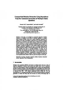
Index Terms— keyword, topic coherence and term significance measure (TCS), support vector machine (SVM) 1. INTRODUCTION With huge quantities of multimedia documents available over the Internet, efficient approaches of indexing, retrieving and browsing these multimedia documents are highly desired. Because all multimedia documents may include audio information that very possibly describes the core concepts of the content, automatic extraction of keywords from such audio information (or spoken documents) will be very useful for the purpose of indexing, retrieving and browsing. This paper proposes unsupervised approaches for keyword extraction from spoken documents, and takes course lectures as the example corpus for experiments [1]. Substantial works have been reported on keyword extraction from texts domain [2, 3, 4], but much less works on spoken documents were reported [5, 6], specially those using information from audio signals such as prosodic features. Previous works proposed an effective supervised approach to extract keywords [7]. However, supervised approaches require substantial labelled data which is difficult to obtain. This paper presents an unsupervised two-stage approach for keyword extraction from spoken documents. The framework is shown in Figure 1. In the first stage, the list of candidate keywords can be initially generated by preprocessing. For each candidate keyword we collect a set of relevant documents, and then compute the topic coherence and term significance measure (TCS) based on the topic similarity among the documents in this relevant document set and the latent topic entropy of the term. This is done with not only the target spoken document archive but web information as well [8, 9]. In the second stage, we utilize the TCS to select positive/negative examples to train an SVM classifier in an unsupervised way, and then this SVM classifier decides the final keyword list.
Here we develop a measure considering both the topic coherence (discussed in section 2.1.1) and the term significance (discussed in section 2.1.2) for unsupervised keyword extraction. Below the document unit is a window size of transcriptions. 2.1.1. Topic Coherence Measure For each candidate keyword ti , first we collect a set of relevant documents from the target spoken archive and form a document set R(ti ). This can be achieved by calculating the probability for a document dj given a term ti as n(ti , dj ) , m=1 n(ti , dm )
P (dj | ti ) = PJ
(1)
where n(ti , dj ) is the occurrence count of the term ti in a document dj and J is the total number of documents. We then collect M documents with higher probabilities in (1) to form the relevant document set R(ti ). Then we train a probabilistic latent semantic analysis (PLSA) model from the target spoken document archive [10]. PLSA is used to analyze the semantics of documents based on the latent topics. PLSA analyzes a set of documents {dj , j = 1, 2, ..., J} and all terms {ti , i = 1, 2, ..., L} they include by defining a set of latent topics {Tk , k = 1, 2, ..., K} to characterize the term-document cooccurrence relationships. For each candidate keyword ti and its relevant document set R(ti ), we then compute the average pairwise cosine similarity for the set R(ti ), P da ,db ∈R(ti ),da 6=db Sim(da , db ) , (2) h(ti ) = |R(ti )|(|R(ti )| − 1) PK k=1 P (Tk | da )P (Tk | db ) qP Sim(da , db ) = qP , (3) K K 2 2 P (T | d ) P (T | d ) a k k b k=1 k=1 where Sim(da , db ) is the cosine similarity between the topic distribution vectors obtained from PLSA for each pair of documents da and db , and |R(ti )| is the total number of documents in R(ti ). In general, a term ti with higher h(ti ) is more likely to be a keyword, because the documents relevant to a keyword usually have similar topic distributions, for example, the term “Iraq” in broadcast news. In contrast, a lower h(ti ) indicates that the relevant documents of term ti have very diverse topic distributions, and very often it is not a keyword, for example, the term “today” in broadcast news. Hence, h(ti ) in (2) is a measure for topic coherence useful for keyword extraction.
Second Stage
First Stage
TCS / WTCS
Candidate Keywords Preprocessing Solution Syllable Summarization …
Spoken Document Archive
Relevant Document Set
Entropy 0.87 Syllable 0.82 : : : : Solution 0.12 Matrix 0.08
Solution 0.12 Syllable 0.82 Summarization 0.65
R(ti) Relevant Document Collection
Web Information (Google, Wikipedia)
PLSA Models
PLSA Training
Positive Examples
Feature Extraction SVM
Negative Examples
Entropy : :
First-Stage Ranking Keyword List
Fig. 1. The framework of two-stage keyword extraction
2.1.2. Term Significance Measure On the other hand, it has been well known that the significance of a term ti can be estimated by the latent topic entropy (LTE) from PLSA [11], E(ti ) = −
K X
P (Tk | ti ) log P (Tk | ti ),
(4)
k=1
where the latent topic distribution for all topics Tk given the term ti , P (Tk | ti ), can be estimated with P (Tk | ti ) =
P (ti | Tk )P (Tk ) , P (ti )
(5)
where P (ti ) can be obtained from a large corpus, and P (Tk ) can be estimated based on P (Tk | dj ) in the target spoken documents. A lower E(ti ) implies the term ti is focused on less latent topics, in other words, carries more topical information or salient semantics. When the consideration of term frequency is included, the significance score of a candidate keyword ti can be defined as P β M m=1 n(ti , dm ) s(ti ) = , (6) E(ti ) where β is a scaling factor, and the score sc (ti ) is inversely proportion to the latent topic entropy E(ti ). 2.1.3. Integrating Topic Coherence and Term Significance Then the topic coherence and term significance measure (TCS) can be computed by putting together (2) and (6), TCS(ti ) = h(ti ) · s(ti ).
(7)
Therefore, TCS(ti ) in (7) considers not only the topic coherence among relevant documents but the significance including latent topic entropy and term frequency. All candidate words are therefore ranked according to TCS(ti ) in the first stage. 2.2. Topic Coherence and Term Significance Measure (TCS) from Web Information The information in the target spoken document archive may be limited. One way to solve the problem is to move to world wide web (WWW), including using Google search engine and the Wikipedia. 2.2.1. TCS-Google We use each candidate keyword ti as the query to the Google search engine and retrieve the top M documents (web pages). We then use all documents retrieved by all candidate keyword as the corpus to train a PLSA model. For each candidate keyword ti we similarly
collect the set of its relevant documents R(ti ) by (1) and calculate the TCS based on Google search engine, TCSg (ti ), using the PLSA model as (7). 2.2.2. TCS-Wikipedia Similarly, for each candidate keyword ti , we first retrieve the top M Wikipedia pages ti refers to. Each retrieved page is regarded as a document, and a PLSA model can be trained. Then we collect the set of relevant documents R(ti ) and obtain TCS based on Wikipedia, TCSw (ti ), in the same way. 2.3. Weighted Topic Coherence and Term Significance Measure (WTCS) We can further integrate the three types of TCS (TCS(ti ), TCSg (ti ), and TCSw (ti )). Google search engine provides a wide variety of documents from different sources but may be noisy. Wikipedia offers well-organized human knowledge but relatively limited. These two resources are complementary to the target spoken document archive, so we linearly interpolate TCS scores from the three to give a Weighted TCS (WTCS) score, WTCS(ti ) = w TCS(ti ) + wg TCSg (ti ) + ww TCSw (ti ),
(8)
where w + wg + ww = 1. w, wg , and ww can be chosen by a development set. 3. SECOND-STAGE KEYWORD EXTRACTION In this stage, we use the first-stage results to train an SVM classifier that decides if each term is a keyword. The input of the SVM classifier is the features for each term, and the output is keyword (+1) or non-keyword (−1). We first rank all candidate keywords ti according to their scores WTCS(ti ) in (8) computed in the first-stage. Then we simply assume the top Q candidate keywords to be positive examples (+1) and the bottom Q candidate keywords to be negative examples (−1), and we use these selected examples to train the SVM classifier. Finally, we use this SVM classifier to label all candidate keywords (including the selected examples) with keyword (+1) or non-keyword (−1). The features for SVM classifier training include three different sets: prosodic features, lexical features, and semantic features [7]. These features are summarized below. 3.1. Prosodic Features Substantial works demonstrated that prosodic information is useful for information extraction from spoken documents [7, 12]. For each
term, only the prosodic features for it when it was produced at the first time in the target archive were used. Twelve prosodic features was used and presented below. 3.1.1. Duration Related Features We assume the keywords may be produced with longer duration. Because different phonetic units have quite different durations, we first compute the average duration of each phonetic unit using the target spoken document archive. For each phonetic unit in a term, we then normalize its duration by its average value. For each term, we then use the maximum, minimum, mean and range of the normalized values for its component units as the four features for the term. 3.1.2. Pitch Related Features We assume the keywords may be produced with wider pitch range. We extract F0 features for frames of each term from the audio data. To avoid discontinuity of pitch contours, we use conventional approaches to smooth them [13]. We also take the maximum, minimum, mean and range of the pitch values for the frames of each term as its four features. 3.1.3. Energy Related Features We assume the keywords may be produced with higher energy. For each frame, we take the value of the 0-th cepstral coefficient as the energy. The maximum, minimum, mean and range are then extracted from the frames of each term as its four features. 3.2. Lexical Features We extract useful lexical features from the transcriptions. The features include TF, IDF, TF-IDF, PoS tags, and left context variation. We assume that the number of different words appearing on the left context of a keyword is limited, such as “on”, “using”, “of” and “is”, while this number for a normal term is usually much larger. Therefore we define a left context variation feature to be the number of different words appearing to the left of the term in the transcriptions. We also normalize it by its term frequency as an additional feature. 3.3. Semantic Features PLSA offers various semantic features. The latent topic entropy E(ti ) in (4) for a term ti is used as a feature here, and another two sets of features introduced below are also useful. 3.3.1. Latent Topic Probabilities The probabilities for each latent topic Tk given each term ti , P (Tk | ti ), as in (5) carry important semantic information. We compute the mean, variance, standard deviation, variance normalized by mean, and standard deviation normalized by mean for these probabilities P (Tk | ti ) for different latent topics given a term ti as the features. 3.3.2. Latent Topic Significance Latent Topic Significance [11] for a given term ti with respect to a latent topic Tk is defined as PJ j=1 n(ti , dj )P (Tk | dj ) Sti (Tk ) = PJ . (9) j=1 n(ti , dj )[1 − P (Tk | dj )] In the numerator of (9), the count of the given term ti in each document dj , n(ti , dj ), is weighted by the likelihood that the given topic Tk is addressed by the document dj , P (Tk | dj ), and then summed over all documents dj in the corpus. Therefore the numerator is the total count of the given term ti used in the given topic Tk over the whole training corpus, as estimated by PLSA model. The denominator is very similar except for latent topics other than Tk , so
P (Tk | dj ) is replaced by [1 − P (Tk | dj )]. We compute the mean, variance, standard deviation, variance normalized by mean, and standard deviation normalized by mean of Sti (Tk ) for different latent topic Tk given a term ti as features. 4. EXPERIMENTS 4.1. Experimental Setup The experiments in this research were performed over a corpus of lectures for a course offered in National Taiwan University. The lectures were given in the host language of Mandarin Chinese but with almost all terminologies produced in the guest language of English. The lecture is 45.2 hours long. The two acoustic models for Mandarin and English were respectively obtained from the ASTMIC corpus and the Sinica Taiwan English corpus, and were adapted by 25.2 minutes corpus from the target speaker (the course instructor). The language model was trained by two other courses offered by the same instructor and adapted by the course slides. The accuracies for the ASR transcriptions were 78.15% for Mandarin characters, 53.44% for English words, and 76.26% for overall. In order to generate the reference keywords, we recruited 61 students who had taken the course as subjects to annotate the keywords for the corpus. Since different subjects annotated quite different sets of keywords of different numbers, we assigned a score of 1/N to a word if it was annotated by a subject who labelled a total of N keywords. We then sorted the terms by their total scores assigned by the 61 subjects, and selected the top N of them as the reference keywords, where N is the integer closest to the average of N for all subjects. In this way, a total of 95 words were generated as the reference keyword list. In the following experiments, we used 1/10 of the lecture transcriptions as the development set to tune the parameters. The candidate keywords were all the words appearing in the target spoken archive with TF-IDF higher than a threshold. 4.2. Evaluation and Discussion 4.2.1. Results of First-Stage Keyword Extraction First we computed TCS scores from three different resources, lecture corpus (TCS-Target), Google (TCS-Google), and Wikipedia (TCSWikipedia), and the N candidate words with highest scores were selected as keywords. The results using ASR transcriptions and manual transcriptions are respectively listed in Table 1. The baselines for keyword extraction to be compared with here are conventional TF-IDF and K-means exemplar. TF-IDF is the approach selecting N terms with highest TF-IDF scores as keywords, which is the basic baseline; K-means exemplar uses K-means algorithm to cluster candidate terms based on feature vectors in latent topic space, and selects exemplars of the clusters as keywords, which is better than some other unsupervised approaches [7, 14]. For ASR transcriptions, TCS-Target, TCS-Google, and TCSWikipedia performed better than TF-IDF but worse than K-means exemplar for F-measure. Considering the three TCS scores with only one resource, TCS-Target performed the worst, but TCS-Google and TCS-Wikipedia provided the better recall and precision respectively. Therefore, WTCS integrating all the three different resources together as in (8) performed the best in comparison with ones using only a single resource. However, the F-measure of WTCS was still lower than the second baseline, K-means exemplar, but the precision of WTCS was the highest among all the approaches. Since the second-stage approach needs correct training examples, the result with higher precision can provide better selection of training exam-
Manual
ASR
4.2.2. Results of Two-Stage Keyword Extraction We then applied second-stage SVM classification using different first-stage scores; the training examples for the SVM classification were from TF-IDF, TCS-Target, or WTCS 1 . The results are shown in Table 2. With the second-stage SVM classification, the performance could be improved regardless of the approaches used in the firststage for both ASR and manual transcriptions. Although the SVM in the second-stage used pseudo-labels for training, probably because the precision of first-stage results were good enough, the classifiers trained with pseudo-labels performed well. This also shows that the features used in second-stage are very useful. We can find that second-stage WTCS for both ASR and manual transcriptions performed significantly better than first-stage results. Improvements from the second-stage approach depend on performance of firststage results, since better results from the first stage provided more reliable positive/negative examples, or more accurate pseudo-labels. Next, we compare the best results from second-stage with Kmean exemplar. For ASR transcriptions, although Table 1 shows that the F-measure of first-stage WTCS was better than TF-IDF but worse than K-means exemplar, second-stage WTCS performed better than the two baselines because of higher precision of first-stage WTCS. For manual transcriptions, the first-stage WTCS was already better than two baselines in Table 1, and applying second-stage approach improved the performance more significantly; also, the improvements was larger than for ASR transcriptions. Finally, we compare the proposed two-stage approach with the results of the supervised approach, which trained the classifier using correct labels and is considered to be the upper bound of the proposed approach. We find that for ASR transcriptions the correctiveness of psuedo-labels is the bottleneck for improvement since the 1 K-means exemplar is to extract exemplar of each cluster, which cannot provide scores needed by the second-stage for the term.
ASR
Table 1. Performance of first-stage keyword extraction (%) Approach Precision Recall F-measure TF-IDF 34.00 18.09 23.61 K-means Exemplar 40.28 30.53 34.73 TCS-Target 35.29 19.15 24.83 TCS-Google 35.94 24.47 29.11 TCS-Wikipedia 40.43 20.21 26.95 WTCS 46.81 23.40 31.21 TF-IDF 41.67 31.91 36.14 K-means Exemplar 49.32 37.89 42.86 TCS-Target 39.45 45.74 42.36 TCS-Google 42.71 43.62 43.16 TCS-Wikipedia 43.21 37.23 40.00 WTCS 50.68 39.36 44.31
performance still needs more effort to be improved compared with supervised result. For manual transcriptions, the positive/negative examples were accurate enough to train a good classifier, and after second-stage approach the F-measure of WTCS increased from 44.31% to 57.80%. The performance was comparable to the supervised result. Table 2. Performance of two-stage approaches (%) Approach Precision Recall F-measure 1st-Stage 34.00 18.09 23.61 TF-IDF 2nd-Satage 17.99 45.74 25.83 1st-Stage 35.29 19.15 24.83 TCS-Target 2nd-Satage 31.88 23.40 26.99 1st-Stage 46.81 23.40 31.21 WTCS 2nd-Satage 43.48 31.91 36.81 K-means Exemplar 40.28 30.53 34.73 Supervised 63.08 51.25 56.55 1st-Stage 41.67 31.91 36.14 TF-IDF 2nd-Satage 27.94 93.62 43.03 1st-Stage 39.45 45.74 42.36 TCS-Target 2nd-Satage 37.40 52.13 43.56 1st-Stage 50.68 39.36 44.31 WTCS 2nd-Satage 50.81 67.02 57.80 K-means Exemplar 49.32 37.89 42.86 Supervised 75.68 58.95 66.27 Manual
ples to train a better classifier. Thus, this justifies the use of WTCS as our first-stage approach. For manual transcriptions, the performance of the results were better than the corresponding results for ASR transcriptions. Considering the three TCS scores with only one resource, TCS-Target performed the worst, TCS-Google performed the best in terms of F-measure, but TCS-Wikipedia provided the highest precision probably because Wikipedia includes well-organized human knowledge. Therefore, WTCS gave the best performance for both F-measure and precision because of integrating advantages from three different resources. For manual transcriptions, WTCS was better than not only TF-IDF but K-means exemplar for F-measure.
5. CONCLUSIONS This paper proposes an unsupervised two-stage keyword extraction approach, first utilizing topic coherence and term significance measure to select training examples, and then using these examples to train an SVM classifier to select the keywords. The experiments over course lectures showed very good keyword extraction performance. 6. REFERENCES [1] [2] [3] [4] [5] [6] [7] [8] [9] [10] [11] [12] [13] [14]
S. Kong and et al, “Learning on demand - course lecture distillation by information extraction and semantic structuring for spoken documents,” in ICASSP, 2009. A. Hulth and et al, “Automatic keyword extraction using domain knowledge,” in CICLing, 2004. Y. HaCohen-Kerner and et al, “Automatic extraction and learning of keyphrases from scientific articles,” in CICLing, 2005. P. D. Turney, “Learning algorithms for keyphrase extraction,” in Information Retrival, 1999. F. Liu and et al, “Automatic keyword extraction for the meeting corpus using supervised approach and bigram expansion,” in SLT, 2008. F. Liu and et al, “Unsupervised approaches for automatic keyword extraction using meeting transcripts,” in NAACL, 2009. Y. Chen and et al, “Automatic key term extraction from spoken course lectures using branching entropy and proodic/semantic features,” in SLT, 2010. O. Kurland and L. Lee, “Pagerank without hyperlinks: structural reranking using links induced by language models,” in SIGIR, 2005. D. Zhou and et al, “Dual-space re-ranking model for document retrieval,” in Computational Linguistics, 2010. T. Hofmann, “Probabilistic latent semantic analysis,” in the 15th Conference on University in AI, 1999. S. Kong and L. Lee, “Semantic analysis and organization of spoken documents based on parameters derived from latent topics,” in IEEE Trans. on Audio, Speech, and Language Processing, 2011. J. J. Zhang and et al, “Improving lecture speech summarization using Rhetorical Information,” in ASRU, 2007. W. Lin, “Tone recognition for fluent mandarin speech and its application on large vocabulary recognition,” in M.S. thesis, NTU, 2004. Z. Liu and et al, ”Clustering to find exemplar terms for keyphrase extraction,” in ACL-AFNLP, 2009.