EXTERNAL REPORT SCK•CEN-ER-123 10/EWe/P-24
Update of the near field temperature calculations for disposal of the PAMELA waste types in a monolithbased geological repository
Eef Weetjens
Note prepared by SCK.CEN in the framework of ONDRAF/NIRAS programme on geological disposal, under contract CCHO-20042470/00/00, DS 251-SAF May, 2010
SCK•CEN Boeretang 200 BE-2400 Mol Belgium
IPA-PAS
EXTERNAL REPORT OF THE BELGIAN NUCLEAR RESEARCH CENTRE SCK•CEN-ER-123 10/EWe/P-24
Update of the near field temperature calculations for disposal of the PAMELA waste types in a monolithbased geological repository
Eef Weetjens
Note prepared by SCK.CEN in the framework of ONDRAF/NIRAS programme on geological disposal, under contract CCHO-20042470/00/00, DS 251-SAF May, 2010 Status: Unclassified ISSN 1782-2335
SCK•CEN Boeretang 200 BE-2400 Mol Belgium
© SCK•CEN Studiecentrum voor Kernenergie Centre d’étude de l’énergie Nucléaire Boeretang 200 BE-2400 Mol Belgium Phone +32 14 33 21 11 Fax +32 14 31 50 21 http://www.sckcen.be Contact: Knowledge Centre
[email protected]
RESTRICTED All property rights and copyright are reserved. Any communication or reproduction of this document, and any communication or use of its content without explicit authorization is prohibited. Any infringement to this rule is illegal and entitles to claim damages from the infringer, without prejudice to any other right in case of granting a patent or registration in the field of intellectual property. SCK•CEN, Studiecentrum voor Kernenergie/Centre d'Etude de l'Energie Nucléaire Stichting van Openbaar Nut – Fondation d'Utilité Publique - Foundation of Public Utility Registered Office: Avenue Herrmann Debroux 40 – BE-1160 BRUSSEL Operational Office: Boeretang 200 – BE-2400 MOL
5
Table of contents 1 2
Introduction .............................................................................................................................7 Model Description...................................................................................................................8 2.1 Thermal Source Term......................................................................................................8 2.2 Geometry.........................................................................................................................8 2.3 Parameters, initial and boundary conditions .................................................................10 3 Results ...................................................................................................................................11 4 Conclusions ...........................................................................................................................13 5 REFERENCES......................................................................................................................14
6
7
1
Introduction
This note reports calculations carried out to quantify the temperature evolution in the near field of a hypothetical repository located in the Boom Clay formation at the Mol site, in case of disposal of vitrified radioactive waste and of hulls and end-pieces, originating from the reprocessing activities at the former Eurochemic plant at Dessel. The considered repository concept for these so-called PAMELA waste types is based on the "Monolith category B" design. Heat transport calculations for the three PAMELA waste types HAGALP1, HAGALP2 and HAGALP3 were already performed and reported in SCK•CEN report ER-78 (Raeymaekers et al., 2008). As such, this note complements chapter 3 of aforementioned report. Indeed, some parameters have been updated recently and these are listed and explained below: • • •
thermal conductivity of the Boom Clay decreased; evidence of anisotropy thermal conductivity of concrete slightly decreased projected date of disposal of PAMELA wastes: 2040
The thermal conductivity of the Boom Clay used in previous calculations of Raeymaekers et al. (2008) was assumed to be 1.7 W/mK. This value was recently revised based on results obtained from the ATLAS III experiment. Important conclusions of this experiment were that the Boom Clay’s thermal conductivity is slightly lower than expected and clearly shows anisotropy. This warranted an update of the thermal calculations for the PAMELA waste (specifically HAGALP1) in order to verify that there is no thermal phase associated with this waste type within the current disposal concept1 (Sillen and Weetjens, 2008). Indeed, when the absolute temperature exceeds 25°C, the validity of the nominal values for the Boom Clay transport parameters becomes questionable. According to NIRAS/ONDRAF’s strategic choices, release of radionuclides should be avoided (ONDRAF/NIRAS, 2009a) by means of engineered design options (e.g. a watertight overpack) during this initial thermal period. In the course of 2009, source and expert ranges of the thermal clay properties have been defined. In present calculations, we used the lower limits of the expert ranges for both horizontal and vertical thermal conductivity. As previous planning documents mentioned disposal of the PAMELA waste types from 2030 onwards, now disposal of waste from nuclear liabilities (to which the PAMELA waste belongs) is foreseen to start in 2040 (ONDRAF/NIRAS, 2009b). This means that the waste is allowed to cool a decade longer. For sake of completeness, both results for disposal in 2030 and disposal in 2040 are shown. A 3D model has been built in order to demonstrate the effect of anisotropy of the Boom Clay. This calculation was compared with results of a 2D axisymmetric model in which an average value of the thermal conductivity was implemented. Calculations were performed with the finite element tool COMSOL Multiphysics version 3.5a (COMSOL, 2008) and results of the 2D axisymmetric model were verified with PORFLOW (Runchal, 1997) calculations.
1
A thermal phase is a period for which the host rock temperature lies above the range within which nominal radionuclide migration properties can be relied on. Currently the maximum temperature at which nominal values of the radionuclide migration parameters are applicable is taken at 25°C.
8
2
Model Description
2.1
Thermal Source Term
The evolution with time of the total thermal power emanating from the waste is demonstrated in Figure 1 for disposal in 2030 (left) and disposal in 2040 (right). Since the inventory dates from 1 January 1996 (Raeymaekers et al., 2008), a cooling period of respectively 34 and 44 years have been taken into account. The calculations revealed that the nuclides 90Sr, 90Y, 137Cs, 137mBa and 241 Am are the major contributors to the decay heat. Furthermore it can be seen that the waste packages of class HAGALP1 generate the most heat. 3.0E+09
3.0E+09 HAGALP1
HAGALP2
2.0E+09
1.5E+09
1.0E+09
2.0E+09
1.5E+09
1.0E+09
5.0E+08
5.0E+08
0.0E+00 1.0E-01
HAGALP3
2.5E+09 decay heat generation [J/WP.a]
2.5E+09 decay heat generation [J/WP.a]
HAGALP1
HAGALP2 HAGALP3
1.0E+00
1.0E+01
1.0E+02
1.0E+03
Time after projected disposal date (2030) [a]
1.0E+04
0.0E+00 1.0E-01
1.0E+00
1.0E+01
1.0E+02
1.0E+03
1.0E+04
Time after projected disposal date (2040) [a]
Figure 1: Thermal source evolution from 2030 (left) and from 2040 (right)
2.2 Geometry To represent the waste packages in the model, the same methodology was adopted as in Raeymaekers et al. (2008). This involved application of cylindrical shapes in order to simplify the geometry of the calculation and homogenisation of the source region using uniform parameters. The actual spatial distribution of the heat source is not believed to have a significant influence on the results.
9
Ø300
1480 2800
concrete monolith
backfill
waste package
homogenised source 14-11-07 GEO-FIG-0682
Figure 2: Homogenisation and simplification of source region (monolith design for HAGALP1)
In order to include the effect of anisotropic behaviour of the Boom Clay, a 3D model was built using the Earth Science Module of COMSOL Multiphysics 3.5a (COMSOL, 2008). The dimensions of the EBS components are stated below. The extent of the Boom Clay was taken 50 m. Table 1: geometry data used in the models
monolith external diameter [m] monolith internal diameter [m] monolith length# [m] waste package height [m] internal gallery diameter [m] external gallery diameter [m]
HAGALP1 2.800 1.480 2.880 1.200 1.500 1.800
HAGALP2 2.800 1.480 2.880 1.346 1.500 1.800
HAGALP3 2.800 1.480 2.880 1.346 1.500 1.800
#
standardised monolith length taken from ANNEX 1 to ONDRAF/NIRAS report “B&C Concept and Open Questions” (Wacquier and Van Humbeeck, to be published)
For symmetry reasons, the modelled domain could be reduced to a quadrant section. A view of the near field 3D geometry is shown in Figure 3. This figure also shows the geometry used in a more simplified 2D axisymmetric model, that was developed in parallel in order to compare isotropic and anisotropic heat transport through the Boom Clay. The mesh settings for both calculations were set to “extra fine”.
Boom Clay
monolith
waste
Bo om ga lle Clay ry lin m ing on o li wa th ste
10
lining
Figure 3: 3D view of the geometric representation of the engineered barriers (left) and simplified 2D axisymmetric geometry (right)
2.3
Parameters, initial and boundary conditions
Heat transport can occur through several processes: conduction, convection and radiation. After emplacement of the monoliths in the disposal galleries, void spaces will be backfilled with cementitious materials and the near field will become quickly saturated with pore water. In such a system, radiative heat transfer is not relevant. It is expected that convection can be excluded as well since the hydraulic conductivities of all EBS materials should be very low, i.e. in the same order as the hydraulic conductivity of the host formation (Kv =2.1×10⁻¹² m/s). This means that heat transfer through conduction only has to be modelled. The energy balance equation in a 3D system is given by:
∂T λ = ∂t ρ s C p
⎛ ∂ 2 T ∂ 2T ∂ 2 T ⎞ ⎜⎜ 2 + 2 + 2 ⎟⎟ + S T ∂y ∂z ⎠ ⎝ ∂x
(1)
Where T (K) denotes temperature, ST is the heat source term, λ (W/(m×K)) is the thermal conductivity, ρs (kg/m3) is the solid density and Cp (J/(kg×K)) the specific heat. The values of these parameters for the different materials in the model are given in Table 2. The parameters for the clay region assume that the material is fully saturated. The applied parameter values for the horizontal and vertical thermal conductivity correspond to the lower limits of the expert range as defined in the SFC1 datasheet v1.3 (https://nirond-km.be/gm/folder1.11.315498 accessed on 18/12/2009). Values for the other parameters and materials are not taken up in this datasheet. Note that for the 2D axisymmetric calculation, an average value for λ of 1.45 W/(m×K) has been used. This value was formerly applied in the updated thermal calculations for disposal of high-level waste and spent fuel (Weetjens, 2009). The concrete monolith has been given the same thermal conductivity and heat capacity values as those of the gallery lining. These values, as well as the parameter values for the backfill were taken from (Weetjens, 2009).
11
The applied thermal parameters for the waste zone comprising the cementitious backfill and matrix materials (glass matrix for HAGALP1 and HAGALP2, cementitious matrix for HAGALP3) are arbitrary. Since both types of matrix materials are not characterised in terms of their thermal properties, a high thermal conductivity and a low thermal capacity are conservatively assumed.
Table 2: Thermal parameters
waste and canister concrete monolith cementitious backfill concrete lining Boom clay
ρs [kg/m3] 5000 2400 2400 2400 2650
Cp [J/kg·K] 500 880 880 880 1094
λ [W/m·K]
λh [W/m·K]
λv [W/m·K]
40 1.5 1 1.5 1.45
1.65
1.25
Initially, the temperature is set equal to 16°C (289.15 K). Zero-flux boundary conditions were applied at the symmetry axes through the repository and the two axial boundaries, while the outer boundaries were chosen far enough not to influence the results.
3
Results
The temperature in the near field is shown in Figure 4 for disposal of HAGALP1, which is the hottest PAMELA waste type, at five years after disposal. The plot corresponds to a cross-section through the centre of the monolith. The interface between the gallery lining and the host formation is represented by the black line. Temperatures at that level are still far from the thermal phase limit (25°C). However, peak temperatures occur somewhat later: at about ten years after disposal (see orange curve in Figure 5). As can be seen in Figure 4, the effect of anisotropy in the Boom Clay zone is hardly noticeable. This is to be expected on short time scales, especially since the values of the thermal conductivities in vertical and horizontal direction differ only by factor 1.32. Figure 5 shows the temperature evolution for HAGALP1 waste at different positions within the near field and clay. The effect of anisotropy remains fairly limited (in the figure at one meter depth in the Boom Clay). Figure 6 shows the temperature evolution at the interface of the concrete lining and the Boom Clay for all considered waste types. It is clear that the maximum allowable temperature (25°C) in the Boom Clay is not exceeded, even when considering that disposal may start already from 2030 onwards. Figure 6 also shows a comparison with results from the simplified (isotropic) 2D axisymmetric calculation. The results based on the selected value of λ, i.e. 1.45 W/(m×K) seem to correspond very well with the 3D anisotropic case. Note that this simplification is valid only for short timescales and short distances. The 2D calculation was verified by benchmarking with PORFLOW (Runchal, 1997). Results of this benchmark showed a good correspondence (results not shown).
12
5
5
HAGALP1 (5 years after disposal in 2040)
HAGALP1 (5 years after disposal in 2030)
4.5
4.5
4
4
3.5
3.5
3
3
2.5
2.5
2
2
1.5
1.5
1
1
0.5
0.5
0
0 0
0.5
1
1.5
2
2.5
3
3.5
4
4.5
5
0
0.5
1
1.5
2
2.5
3
3.5
4
4.5
5
26 25.5 25 24.5 24 23.5 23 22.5 22 21.5 21 20.5 20 19.5 19 18.5 18 17.5 17 16.5 16
28
28
27
27
26
26
25
25
24
24
temperature [°C]
temperature [°C]
Figure 4: temperature field in the near field 5 years after disposal: cross section through the centre of a monolith containing HAGALP1 waste. Disposal starts at 2030 (left) or 2040 (right)
23 22 21
23 22 21
20
20
19
19
18
18
17
17
16
waste monolith concrete backfill lining interface Boom Clay 1m deep into Boom Clay (horizontal) 1m deep into Boom Clay (vertical)
16 0
10
20
30
40
time after disposal (2030) [a]
50
60
0
10
20
30
40
50
60
time after disposal (2040) [a]
Figure 5: temperature evolution for disposal of HAGALP1 waste at various positions in the repository near field, for disposal at 2030 (left) and 2040 (right) respectively.
13
26
26 NF temperature criterion
NF temperature criterion
25
24
24
23
23
temperature [°C]
temperature [°C]
25
22 21 20
22 21 20
19
19
18
18
17
17
16
HAGALP1 (3D) HAGALP2 (3D) HAGALP3 (3D) HAGALP1 (2D) HAGALP2 (2D) HAGALP3 (2D)
16 0
10
20
30
40
time after disposal (2030) [a]
50
60
0
10
20
30
40
50
60
time after disposal (2040) [a]
Figure 6: Temperature evolution at interface gallery lining - Boom Clay layer for a 3D anisotropic case and a 2D axisymmetric, isotropic case.
For completeness, Table 3 gives the calculated maximum temperatures, Tmax, and corresponding times for the waste types under study. Table 3: Peak temperatures, Tmax [°C] and times [a] at interface gallery lining - Boom Clay for disposal in 2030 (upper) or 2040 (lower)
Disposal at 2030 HAGALP1 HAGALP2 HAGALP3 Peak Temperature, Tmax [°C] 22.86 17.84 16.49 Temperature increase, ∆T [°C] 6.86 1.84 0.49 Time [a] 12 13 22 Disposal at 2040 HAGALP1 HAGALP2 HAGALP3 Peak Temperature, Tmax [°C] 21.46 17.47 16.43 Temperature increase, ∆T [°C] 5.46 1.47 0.43 Time [a] 12 11 23
4
Conclusions
The results of the updated heat transport calculations indicate that for the considered repository concept based on the monolith category B design the maximum temperature increase attained at the interface between the gallery lining and the Boom Clay does not exceed 6.9 °C even for the most active waste type, i.e. HAGALP1 considering disposal in 2030. Based on the current planning of NIRAS/ONDRAF, it is likely that disposal of the PAMELA waste forms will only start in 2040. Consequently, it is not considered necessary to adapt the current monolith design for these waste types. A comparison between 3D anisotropic case and a simplified 2D geometry has shown that when one is interested in the temperature evolution at short distances (interface) and short timescales (time of peak), the average value of the thermal conductivity (1.45 W/(m×K) can be used. This also supports the results obtained in SCK•CEN report ER-86 (Weetjens, 2009) for which no full 3D assessment has been made at the time.
14
5
REFERENCES
COMSOL (2008) COMSOL Multiphysics 3.5a, Earth Science Module, COMSOL AB, Stockholm, Sweden. ONDRAF/NIRAS (2009a) The Long-term Safety strategy for the Geological Disposal of Radioactive Waste, second full draft, ONDRAF/NIRAS report NIROND-TR 2009-12E. ONDRAF/NIRAS (2009b) The Plan for the Safety and Feasibility Case 1, first full draft, ONDRAF/NIRAS report NIROND-TR 2009-13E. Raeymaekers, F., Weetjens, E. and Marivoet, J. (2008) Geological disposal of PAMELA and compacted structural and technological waste: Radiological consequences in the case of the expected evolution scenario. SCK•CEN report ER-78. Runchal A.K. (1997) PORFLOW: A Multifluid Multiphase Model for Simulating Flow, Heat Transfer and Mass Transport in Fractured Porous Medium, User's Manual – Version 3.07. ACRi Inc., Bel Air, California. Sillen X. and Weetjens, E. (2008) A definition of thermal phase: proposal and suggested use. ONDRAF/NIRAS note 2008-0911. Wacquier W. and Van Humbeeck H. (draft version March 2009) B&C Concept and Open Questions. ONDRAF/NIRAS report ref. 2009-0146. Weetjens, E. (2009) Update of the near field temperature evolution calculations for disposal of UNE-55, MOX-50 and vitrified HLW in a supercontainer- based geological repository. SCK•CEN report ER-86.