promote a more constant horizontal velocity for the runner. This paper addresses ... performed three trials on a treadmill, one at a "slow" speed of 3.8 m/s, one ... Figure 1. In the small time interval 2At (2 frames), tbe segment moves from po- ...... arms when one walks on a railroad track or skates on ice for the first time, but.
INTESNATIONAL JOURNAL OF SPORT BIOMECHANICS, 1967, 3, 242-2&3
Upper Extremity Function in Running. II: Angular Momentum Considerations Richard N. Hinrichs Ten male recreational runners were filmed using three-dimensional cinematography while running on a treadmill at 3.8 m/s. 4.5 m/s. and 5.4 m/s. A 14-segment mathematical model was used to examine the contributions of the arms to the total-body angular momentum about three orthogonal axes passing through the body center of mass. The results showed that while the body possessed varying amounts of angular momentum about all three coordinate axes, the arms made a meaningful contribution to only the vertical comfK)nent (H^). The arms were found to generate an alternating positive and negative H^ pattem during the running cycle. This tended to cancel out an opposite H^ pattern of the legs. The trunk was found to be an active participant in this balance of angular momentum, the upper trunk rotating back and forth with the arms and, to a lesser extent, the lower trunk with the legs. The result was a relatively small total-body H^ throughout the running cycle. The inverse relationship between upper- and lower-body angular momentum suggests that the arms and upper trunk provide the majority of the angular impulse about the z axis needed to put the legs through their alternating strides in running. In searching the literature on the biomechanics of running, one can find only an occasional mention of the arms and the role they play in the running process. It appears that little importance has been placed on the arm swing. In the opinion of Mann (1981) and Mann and Herman (1985), for example, the arms are simply used for balance and do not play a significant role in influencing the quality of running performance. However, the present study will show that the arms serve a substantially greater purpose than simply maintaining balance in running. This is the second in a two-article sequence. In the first paper (Hinrichs, Cavanagh, & Williams, 1987), the arms were shown to provide lift and promote a more constant horizontal velocity for the runner. This paper addresses the angular momentum aspects of the arm action in running. Because the arms are not an isolated system, the angular momentum of the arms will be described in relation to that of the legs and of the head and trunk.
Richard N. Hinrichs is with the Exercise and Sport Research Institute, Department of Health and Physical Education. Arizona State University. Tempe. AZ 85287. 242
RUNNiNC: ANGULAR MOMENTUM
243
Procedures Ten male recreational runners ranging in age from 20 to 32 years (M = 22.5 years) were used as subjects. They ranged in height from 1.61 to 1.83 m (M = 1.76 m), and ranged in mass from 51.3 to 75.9 kg (M = 64.8 kg). Each subject performed three trials on a treadmill, one at a "slow" speed of 3.8 m/s, one at a "medium" speed of 4.5 m/s, and one at a "fast" speed of 5.4 m/s. These represented running paces of 7, 6, and 5 minutes per mile, respectively. A fourcamera three-dimensional (3D) cinematographic technique was employed using the DLT algorithm (Abdel-Azis & Karara, 1971). Each camera operated at a nominal rate of 100 frames/s. Body Segment Parameters A 14-segment mathematical model of the body was used and consisted of the head, trunk, both upper arms, forearms, hands, thighs, calves, and feet. The 3D estimates of joint centers digitized from the films represented the endpoints of each segment (Hinrichs et al., 1987). An exhaustive set of anthropometric measures was taken on each subject to aid in the estimation of body segment parameters (BSPs). These measurements were used to predict segment masses, centers of mass (CM), and moments of inertia for each subject using four different combinations of BSP data from the literature. These four combinations are as follows: 1. Masses and CM from the regression equations of Clauser, McConville, and Young (1969), moments of inertia from the regression equations of Hinrichs (1985) based on the data of Chandler, Clauser, McConville, Reynolds, and Young (1975). 2. Masses and CM from the regression equations of Clauser et al. (1969), moments of inertia from the mean data of Whitsett (1963) corrected for height and body mass differences according to the method of Dapena (1978). 3. Masses and CM from the mean data of Clauser et al. (1969), moments of inertia from the mean data of Whitsett (1963) corrected for height and body mass differences according to the method of Dapena (1978). 4. Masses, CM, and moments of inertia from the regression equations of Zatsiorski and Seluyanov (1985). The set of BSP data that best produced constancy of airborne angular momentum and horizontal linear momentum were chosen for each subject. Details about the selection of BSP are included in Hinrichs (1982).
Smoothing and Differentiating The raw 3D segment endpoint data were smoothed using a second-order Butterworth digital filter (Winter, Sidwalt, & Hobson, 1974) with cutoff frequencies ranging from 2 to 8 Hz. Different cutoff frequencies were chosen objectively for each coordinate of each endpoint using an algorithm similar to the one described by Jackson (1979) adapted for use with a digital filter. The vertical (Z) coordinates of segment endpoints were generally found to need higher cutoff frequencies for smoothing than did the X or Y coordinates.
244
HINRICHS
Due to the laborious nature of the 3D cine process, only one complete running cycle per trial was digitized for each subject. An additional 10 frames were digitized at the beginning and end of each trial to reduce endpoint effects ofthe digital filter. Finite differences (Miller & Nelson, 1973) were used whenever the analysis called for taking the first or second time derivative of the smoothed displacement data. No further smoothing was done following differentiation.
Algorithm for Computing Angular Momentum The smoothed 3D coordinates ofthe segment endpoints were entered into a computer program that calculated the angular momentum of individual body segments and systems of segments about the body center of mass. The method used to compute angular momentum is similar to the method of Dapena (1978). Each segment was assumed to be symmetrical about its longitudinal (long) axis. Thus, any transverse axis through the segment CM became a principal axis of inertia for the segment. Rotations about segment long axes, with the exception of the trunk segment, were ignored. This was accomplished mathematically by setting all nontrunk segment moments of inertia about their long axes equal to zero. Dapena (1978) has shown this procedure to involve little error in the calculation of human body angular momentum. Nontrunk Segments. Consider, for example, the body segment shown in Figure 1. In the small time interval 2At (2 frames), tbe segment moves from positioni-1 through position i to position i-t-l relative to a noninertial B:xy2 refer-
Path of segment CM relative to B
Figure 1 — Computii^ angular momentuin of a body segment about the body center of mass (point B).
RUNNING: ANGULAR MOMENTUM
245
ence frame translating with the body CM (point B). The B:xyz reference frame does not rotate but remains parallel to the fixed O:XYZ reference frame. The segment possesses two forms of angular momentum about point B: "local," which is inherent in the rotation of the segment about a transverse axis through its own CM, and "remote," which is inherent in the translation of the segment CM (point C) relative to the body CM (Hopper, 1973). Local angular momentum requires the calculation of the segment's angular velocity vector, w. First, an instantaneous plane of rotation is established. The unit vector DJ normal to this plane in the direction of the angular velocity is ni = (Li_i X Li+,)/|Li_i X Li^il
(1)
where L j . ^ and Lj_^[ are the vectors defining the segment long axis (proximal to distal) at frames i - 1 andi-l-1, respectively. The angular displacement, 6^, of the segment during tbe time interval 2At is ffi = sin-' [(lLi_i X Li+,|)/(|Li_i| m+jl)]
(2)
The angular velocity vector at frame i is therefore (3) Because the axis of rotation of the segment is a principal axis of inertia, the local angular momentum vector is parallel to the angular velocity vector, (HL);
= ^
(4)
where (H^); is the segment local angular momentum vector at frame i, I is the segment's moment of inertia about a transverse axis through its CM, and wj is the angular velocity vector at frame i. The remote angular momentum of the segment is simply the moment of the linear momentum of the segment expressed in a reference frame translating with the body CM. Thus (HR);
= Fj X mf-i
(5)
where (Hjt)^ is the segment remote angular momentum vector at frame i, TJ is the vector locating the segment CM relative to the body CM at frame i, m is the segment mass, and TJ is the time derivative of the vector TJ. The total angular momentum of the segment about the body CM at frame i is the sum of the local and remote terms, (H)i =
(HL).
+
(HR);
(6)
Trunk Segment. Equation 6 was used for the trunk segment rotations in the sagittal and frontal planes. Here the entire trunk was considered a cylinder rotating about a transverse axis. (Note that the term transverse axis shall refer to any axis that is perpendicular to the segment's longitudinal axis.) The rotation of the trunk about its long axis was also considered, however. The presence of two shoulder and two hip landmarks permitted the estimation of this component of angular momentum. The shoulder and hip points also allowed the trunk to be
246
HINRICHS
subdivided into an upper trunk and a lower trunk, each having its own local angular momentum about their common longitudinal axis. The nature of the calculations did not require a plane of separation of the upper and lower trunk. The upper trunk was assumed to rotate with the shoulders, the lower trunk with the hips. The method for calculating the angular momentum of the upper trunk about the trunk long axis is outlined below. The procedure for the lower trunk is identical to that of the upper trunk with the right and left hip points being substituted for the right and left shoulders, respectively. The procedure starts by defining the trunk long axis vector (L) at each of the three frames, i - 1 , i, and i-!-l (see Figure 2). An auxiliary "nql" reference fi-ame is defined by the unit vectors n, q, and I, and rotates with the trunk long axis frame i - 1 to i + 1 . The vector \ is the unit vector along the trunk long axis at each frame. The unit vector n is normal to the plane of rotation of the trunk long axis between frames i - 1 and i + 1. It is defined according to equation 1 in an identical manner as for all other segments. The auxiliary reference frame rotates about n between frames i - 1 and i + 1. Finally, the unit vector q is defined by the cross-product of I and n.
n _
Rotation of D in nq plane
'-' /1> \
\
Figure 2 — Computing angular momentum of the upper trunk or lower trunk about the trunk long axis.
RUNNING: ANGULAR MOMENTUM
247
Next a vector S locating the left shoulder relative to the right shoulder is defined at each frame. It is the rotation of this vector about the trunk long axis that is of interest here. Because S may not necessarily lie in the nq plane at a given frame, another vector D is defined by the cross-product of L and S. This vector D lies in the nq plane and its rotation in this plane between frames i —1 and i -F1 is representative of the rotation of the shoulders about the trunk long axis during this interval. This rotation can easily be measured if D is first expressed in the auxiliary reference frame. This is done in the following equation: D' = [X]D
(7)
where [X] is the transformation matrix relating the nql reference frame to the XYZ reference frame, and D' is the vector D transformed into the nql reference frame. The angular displacement of the vector D' between frames i - 1 and i -I-1 is then determined by the following equation: 4. = sin-[(|D'i_i X D'i^,|)/(|D'i_i| iD'i^J)]
(8)
where is the angular displacement, and D'j_i and D'j_^j are the vector D' at frames i - 1 and i + 1 , respectively. The direction of the angular displacement depends on whether or not the rotation was counterclockwise { + } or clockwise (~) in the nq plane. This can be detected by looking at the cross-product ofthe vectors D ' j _ | and D'i^j. For this purpose, the unit vector u' was defmed and indicated the direction of the rotation such that u' = (D'i_, X D'i + ,)/|D'i_, X D'i^il
(9)
If the rotation is counterclockwise, u' will have the coordinates (0, 0, 1) expressed in the auxiliary reference frame. If the rotation is clockwise, u' will have the coordinates (0, 0, - 1 ) . If the constant C is set equal to the third coordinate of u', it is then possible to express the angular velocity of the upper trunk about the trunk long axis at frame i by the following equation: (wuT)i = »i C