Urban Landscape Classification System Using

Urban Landscape Classification System Using Airborne LiDAR Matthew A. Carlberg, Peiran Gao, George Chen, Avideh Zakhor Video and Image Processing Lab University of California, Berkeley {carlberg,p gao,gchen,avz}@eecs.berkeley.edu

Abstract The classification of urban landscape in aerial LiDAR point clouds can potentially improve the quality of largescale 3D urban models, as well as increase the breadth of objects that can be detected and recognized in urban environments. In this paper, we introduce a multi-category classification system for aerial LiDAR point clouds. We propose the use of a cascade of binary classifiers for labeling each LiDAR return of an input point cloud as one of five categories: water, ground, roof, tree, and other. Each binary classifier identifies LiDAR returns corresponding to a particular class, and removes them from the processing pipeline. Categories of LiDAR returns that exhibit the most discriminating features, such as water and ground, are identified first. More complex categories, such as trees, are identified later in the pipeline after contextual information, such as the location of ground and roofs, has been obtained, and a significant number of LiDAR returns have already been removed from the pipeline. We demonstrate results on a North American dataset, consisting of 125 million LiDAR returns over 3 km2 , and a European dataset, consisting of 200 million LiDAR returns over 7 km2 . We show that our ground, roof, and tree classifiers, when trained on one dataset, perform accurately on the other dataset1 ..

(a)

1. Introduction 3D urban models have important applications in disaster management, virtual reality, and urban planning. Due to their large scale, the generation of such models requires algorithms that are scalable, efficient, and free of human intervention. Aerial and ground-based LiDAR range finders are most often used to generate these models due to their high accuracy and acquisition speed [6]. Point-wise classification of aerial LiDAR point clouds can guide surface reconstruction techniques in urban modeling. For example, buildings are best modeled using piecewise planar surfaces,

(b)

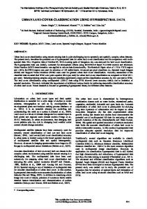
Figure 1: (a) An input colored point cloud from D1 and its (b) labeled version. Ground is white, roofs are red, trees are green, and other points are black. while vegetation is best represented in the point cloud domain. Furthermore, classification of LiDAR point clouds can benefit object recognition tasks in urban environments by providing high-level contextual information. One approach to classifying LiDAR point clouds is to use aerial sensors to label each return as either terrain or offterrain. A comparison of algorithms that use this approach

1

This work is supported with funding from the Defense Advanced Research Projects Agency (DARPA) under the Urban Reasoning and Geospatial ExploitatioN Technology (URGENT) Program. This work is being performed under National Geospatial-Intelligence Agency (NGA) Contract Number HM1582-07-C-0018, which is entitled, Object Recognition via Brain-Inspired Technology (ORBIT). The ideas expressed herein are those of the authors, and are not necessarily endorsed by either DARPA or NGA. This material is approved for public release; distribution is unlimited. Distribution Statement “A” (Approved for Public Release, Distribution Unlimited)

1

can be found in [15], in which it is concluded that complex urban landscapes pose the greatest challenges for classification. More recent work focuses on the extraction of buildings from aerial LiDAR point clouds [3, 17]. Zhang et al. identify terrain and off-terrain points as a pre-processing step, and use region growing segmentation based on planefitting over local neighborhoods in order to extract building footprints [17]. Caceres and Slatton use airborne and ground-based sensors with spin images as features for supervised, non-parametric classification of points on a single building [3]. As a dual to identifying buildings, Secord and Zakhor identify trees in aerial LiDAR point clouds over the city of Berkeley using normalized cut segmentation as a pre-processing step to supervised segment-wise classification [14]. In multi-class classification, aerial LiDAR point clouds are typically labeled using categories such as ground, building, and vegetation. Charaniya et al. perform pixel-wise, four-category classification using expectation maximization with features such as height variation and return intensity, computed over a 2.5D height map [4]. Lodha et al. improve on this work by introducing new features and using AdaBoost [10]. They report results with approximately 90% accuracy over their Santa Cruz dataset. Forlani et al. use two region growing segmentations followed by rule-based, segment-wise classification to identify three classes of LiDAR returns [5]. Their work also remains in the 2.5D domain, reporting results also in the 90% range over the city of Pavia, Italy. Zingaretti et al. [18] present techniques for automatically extracting the rules used by Forlani et al. [5]. Porway et al. parse aerial imagery into multiple categories, including trees, cars, and roofs, by using a statistical framework that takes advantage of a bottom-up objectlevel hierarchy and top-down scene-level contextual relationships [13]. Whereas airborne methods usually reside in the 2.5D domain, methods that use ground-based LiDAR often take advantage of full 3D analysis. Anguelov et al. use Markov Random Fields (MRFs) to classify terrain data obtained from a robot-mounted sensor into the categories of ground, building, tree, and shrubbery [1]. They report 93% accuracy while processing data offline over a dataset with 35 million LiDAR returns. Lalonde et al. use Principle Component Analysis (PCA) on local neighborhoods and a Bayesian classifier to identify ground-based LiDAR returns as planar, scatter, or linear [8]. As a post-processing step, they perform region growing in 3D to connect proximal LiDAR returns of the same category. Their accuracy results are in the 80% range for two relatively complex, yet small, datasets. In this paper, we present a modular and efficient system for labeling each return of an aerial LiDAR point cloud as water, ground, roof, tree, or other. The distinguishing attributes of our system are (a) the use of a cascade of bi-

nary classifiers that frame the multi-category classification problem as a series of simpler sub-problems; (b) the use of region growing in the 3D domain as a means of enforcing spatial coherency; and (c) generalization capability on new datasets for which it has not been trained. The input to our system is an aerial, colored LiDAR point cloud with each return specified by an (x, y, z) position in a global coordinate system and an associated (r, g, b) color value. An example input point cloud and its labeled version are shown in Figs. 1(a) and 1(b) respectively. Our system is composed of a series of cascaded binary classifiers, as shown in Fig. 2. Each binary classifier identifies LiDAR returns corresponding to a particular class and removes them from the processing pipeline. Categories of LiDAR returns that exhibit the most discriminating features, such as water and ground, are identified first. More complex categories, such as trees, are identified later in the pipeline, only after contextual information, such as the location of ground and roofs, has been obtained, and a significant number of LiDAR returns have already been removed from the pipeline. The modularity of our system enables each binary classifier to use its own unique set of discriminating features. The intuition behind the system is that each classifier in the pipeline “peels off” points corresponding to its particular class. LiDAR returns that are positively identified as a particular class are removed from the pipeline, and are used by downstream classifiers only for high level contextual information, as represented by the dashed arrows in Fig. 2. Cascaded classifiers have successfully been used, in a similar way, for face detection [16]. Each binary classifier in our system performs region growing segmentation as a means of enforcing spatial coherency, followed by segment-wise classification. This aspect of our approach resembles that of [14], except that our segmentation and classification work fully in 3D rather than 2.5D. The 3D aspect of our approach resembles that of [8], except that we perform an additional step of segmentwise classification in order to arrive at urban landscape categories. In addition, our work deals with large scale airborne data, rather than small scale terrestrial data [8]. We test our classification system on two different datasets D1 and D2. D1 is a public domain dataset [12], and captures range information over a North American city. It contains approximately 125 million LiDAR returns with an average spatial density of 65 returns/m2 . D2 captures range information over a European city, and contains approximately 200 million LiDAR returns with an average spatial density of 25 returns/m2 . Both datasets are split into 100m × 100m tiles of data. In Section 2, we describe our water classifier; Section 3 includes 3D segmentation and classification for ground, roofs, and trees. We present results in Section 4, and conclude in Section 5.

Figure 2: Classification system is composed of a pipeline of binary classifiers.

2. Water Classifier In this section, we describe our water classifier, the first binary classifier in our cascaded system. The water classifier is first in the pipeline, since out of the five classes, water tends to exhibit the most discriminating features, the most notable of which is low return density as compared to highly scattering non-water areas. Specifically, due to the relative smoothness of water surfaces, incident laser beams are reflected with minimum scattering on water surfaces. As a result, the LiDAR scanner only receives return signals when outbound laser beams are near normal to the water surface. We begin by projecting a 3D point cloud onto a 2.5D depth image consisting of pixels of fixed size in the (x, y) plane. This 2.5D approach is justified considering that the water surfaces of interest typically lack 3D structure due to their fluid nature. In addition, memory and computation requirements are significantly lowered by projecting the 3D point cloud onto a height map while still maintaining features that are characteristic of water areas. Our proposed water classifier works in two steps. In the first step, we perform region growing segmentation on the 2.5D image based on the density of empty pixels with no returns in a neighborhood. In the second step, a trained random forest classifier [2] identifies each segment as either water or non-water. LiDAR returns that are part of segments that are identified as non-water are passed down the pipeline for further processing. The feature vector for a particular segment in our water classifier consists of the segment’s empty-pixel density, absolute height, and size. To compute a segment’s empty-pixel density, we divide the number of empty pixels with no returns in the entire segment by the total number of pixels in the segment. Even though this feature has already been used for region growing, it is still the most discriminating feature between water and non-water segments. We also exploit the fact that water areas are in general the lowest surfaces in the landscape, and use the absolute height of a segment as a feature. This feature helps to distinguish objects such as buildings with large glass rooftops from water surfaces. This is because glass surfaces result in low return density similar to water. Lastly, to avoid misclassifying small patches of non-water areas that have a large empty-pixel density, we use the size, i.e. the number of pixels of a segment, as the third feature. In order to train our random forest classifier, we label 2.5D depth images that have been generated for a subset

of our aerial LiDAR data. Using photo editing software, we identify each pixel as water or non-water. The label for each segment in the training stage is assigned based on a majority vote of pixels in the segment.

3. The 3D Classifiers In contrast to our water classifier, our proposed ground, roof, and tree classifiers treat input LiDAR point clouds as fully three dimensional data, inspired by terrestrial robotics applications. Since modern airborne LiDAR data acquisition systems often collect data in high-density, wide-angled swaths with multiple fly overs, treating the data as three dimensional is justified, if not ideal. The 3D classifiers share a common flow. Each classifier performs a 3D region growing segmentation step grouping together proximal LiDAR returns with similar local point statistics, followed by segment-wise classification.

3.1. Segmentation in 3D Our 3D region growing algorithm is inspired by the saliency features of Medioni et al. [11]. Specifically, we use PCA to analyze the spatial distributions of neighborhoods of points. For each point of the 3D dataset, we first collect all neighbors within a specified radius rpca , which defines the scale of the neighborhood over which spatial analysis is performed. Singular value decomposition of the covariance matrix of the 3D point positions within the neighborhood results in a set of eigenvalues (λmax , λmid , λmin ), and a set of eigenvectors (emax , emid , emin ) for each LiDAR return. As described by Medioni et al. [11], for a neighborhood of scattered points, we expect λmax ≈ λmid ≈ λmin ; for a neighborhood of co-planar points, we expect λmax ≈ λmid >> λmin ; and for a neighborhood of co-linear points, we expect λmax >> λmid ≈ λmin . After PCA, each classifier divides the LiDAR returns of its input into two disjoint subsets based on the resulting eigenvalues. For the ground and roof classifiers, each LiDAR return is tagged as belonging to either a locally planar or non-planar neighborhood. Based on the interpretation of PCA as described above, we define a “planar point” as a point that has λmid /λmin > λplanar , where λplanar is a user-specified threshold. This criteria allows us to implement a simple and robust region growing algorithm as described below based on the assumption that ground and roof points are a subset of planar points. For the tree classifier, each LiDAR return is tagged as belonging to either a

locally scattered or non-scattered neighborhood. A “scatter point” is defined as a point that has λmax /λmid < λscatter1 and λmid /λmin < λscatter2 , where λscatter1 and λscatter2 are two user-specified thresholds. Our region growing algorithm for the tree classifier is based on the assumption that tree points are a subset of scatter points. We now describe the region growing step of our 3D classifiers. For the ground and roof classifiers, we group proximal, planar LiDAR returns into a set of segments, similar to [8]. In the classification stage, described in Section 3.2, a subset of these segments are identified as either ground or roof and the rest of the input, including all non-planar points, are identified as non-ground or non-roof respectively, and passed to the next classifier in the pipeline. In the tree classifier, scatter points are segmented in a similar manner. For 3D segmentation, we grow a region through any pair of points that are within a distance rseg of each other, where rseg is a user-specified parameter.

3.2. Classification 3.2.1. Ground Classifier Our 3D region growing provides a set of locally planar segments in 3D, a subset of which correspond to ground. We use simple heuristics in order to implement a ground classifier that is efficient without using machine learning techniques. Specifically, we have empirically found the most discriminative segment features for ground classification are the median height of a segment and its size in number of LiDAR returns. For an input point cloud, we normalize this 2D feature space using the maximum and minimum height and size values observed in the point cloud. Ideally, one expects the ground segment to be lowest in height and largest in size, among all segments in a sufficiently large region. However, in complex urban settings over a limited area, it is rare to find such a segment. To circumvent this, we first imagine an ideal segment that has the size of the largest segment and height of the lowest segment of the input point cloud. We normalize these features to values between 0 and 1, so that in our normalized feature space, the ideal segment resides at (height, size) location (0, 1). We then compute the Euclidean distance between each segment of the input point cloud and this ideal segment in the feature space, and declare the segment that is closest to the ideal segment as the main ground segment. As described above, we also wish to account for the possibility of multiple ground segments. In general, this is due to the presence of large buildings or river canyons. To account for this, we also identify as ground all segments that are within a factor of 10 in size of the main ground segment, and that have few or no LiDAR returns in the input point cloud at a lower height. This idea of identifying and counting points that fall below a segment is discussed in more detail in Section 3.2.2.

3.2.2. Roof Classifier Once the ground segments are identified in the collection of locally planar 3D segments, most of the remaining segments correspond to roofs, building facades, and cars. Three simple segment-wise features are used by a random forest classifier to identify buildings from these remaining segments. The first is the median height of a segment above ground. Specifically, we subtract the median ground height of an input point cloud from the absolute median height of the segment. As mentioned in Section 1, we allow our classifiers to use results from previous classifiers to add context to our features. Specifically, we assume that the roof classifier has access to all of the LiDAR returns that have already been labeled as ground by the ground classifier so that it can compute the median ground height. The second feature is the normalized count of LiDAR returns that fall underneath a segment. Roofs tend to have a relatively high count of points below them, due to LiDAR returns that fall onto building facades or ground regions directly below rooftops. On the other hand, ground points usually have nothing underneath them. We compute this feature as follows: For each point in the segment, we count all points in a 1m × 1m window in the (x, y) plane surrounding the point that are (a) lower in height and (b) not part of the segment. Using a window of this size ensures that ground regions directly below rooftops influence this feature. We then normalize this point count by the total size of the segment. The third feature is an estimate of the z component of the segment’s normal vector, as estimated by a linear least squares plane fit of all points in the segment. This is intended to remove vertical surfaces such as building facades. To create a training set for our roof classifier, we have developed a visualization tool to generate 3D segment-wise ground truth. Namely, for an input point cloud, our tool allows a human operator to view and tag each 3D segment as ground, roof, tree, other, and none of the above. None of the above includes objects that are unidentifiable, or on which segmentation failed, causing two different classes to be grouped into a single segment. Segments that are labeled as none of the above are not included in training or cross-validation. For the roof classifier, locally planar segments labeled as “roof” are used as the positive examples for training the classifier, and locally planar segments labeled as “other” are used as the negative examples. 3.2.3. Tree Classifier The tree classifier begins from a set of segments composed of all points that belong to locally scattered neighborhoods. From our experiments, we observe that these segments typically correspond to three different types of objects: actual trees, objects on building tops e.g. antennas and building edges, and objects low to the ground e.g. cars. Accordingly, the guiding principle of our tree classifier is to use features that identify trees as objects that are (a) offset

from ground and rooftops and (b) have a point distribution that is non-planar in 3D. Our first segment feature is the normalized count of LiDAR returns that fall below a segment as described in Section 3.2.2. Segments corresponding to cars, for example, should have very few points underneath them, whereas trees tend to have many points that fall below them, because LiDAR often can penetrate trees resulting in returns from the ground below. Our second segment feature is the percentage of points in a segment that are offset from rooftops. Specifically, for each LiDAR return of a segment, we find the closest LiDAR return in the point cloud that is identified as roof. If the distance between the two returns is greater than a threshold, we count the point as offset from roof. This is an example of downstream classifiers using context from upstream classifiers to help differentiate trees ¯ max from rooftop clutter. For the last two features we use λ ¯ ¯ ¯ ¯ ¯ and λmid /λmin , where the values (λmax , λmid , λmin ) are the eigenvalues obtained from PCA over the entire segment. In the same way that LiDAR returns corresponding to trees should be scattered on a local level, they should also be scattered on a larger scale. In essence, these features measure the “scatterness” of each segment as a whole. It is important to note that our tree classifier does not use color as a feature for classification even though trees tend to be green. Our justification for not using color is threefold. First, color data is not always well-registered with the range data, as evidenced in our D1 dataset. Second, color is particularly dependent on illumination, and in urban landscapes shadows are prevalent due to the presence of tall buildings. Third, tree colors tend to be season-specific. The training of our tree classifier is nearly identical to the training of our roof classifier, described in Section 3.2.2. From the segment-wise ground truth, we use locally scattered segments identified as “trees” as the positive examples for training the random forest classifier, and locally scattered segments identified as “other” as the negative examples.

4. Results Figs. 1(b) and 3 demonstrate example results for our entire classification system. For our water, roof, and tree classifiers, we train a random forest model for each dataset. Table 1 provides a description of the training set for each classifier.

4.1. Water Classifier Results For each training set, we build a random forest classifier with 300 decision trees. We split each training set into 10 equally-sized bins, and perform 10-fold cross validation. Average total error, average precision, and average recall for both datasets are reported in the D1 and D2 columns of Table 2. We also apply the random forest classifier as trained on the D2(D1) dataset to test on the D1(D2) training set, as

Dataset

Classifier

Segments in Training Set

Positive Training Examples

Area of Training Set (km2 )

D1 Water 5482 670 0.5 D2 Water 170 47 0.5 D1 Roof 501 458 0.3 D2 Roof 337 295 0.3 D1 3D Tree 1303 600 0.3 D2 3D Tree 1984 995 0.3 D1 2.5D Tree 296,150 124,870 0.2 D2 2.5D Tree 267,950 121,111 0.3 Table 1: Description of Training Set for Each Classifier shown in the D1*(D2*) column of Table 2. These two experiments provide a quantitative measure of the robustness of our classifiers and their generalization capability. As seen in Table 2, our water classifiers for D1 and D2 do not generalize well across datasets. We attribute this to the use of empty pixel density as a segment feature. Whereas a quantity such as the height of a segment is determined by the physical world, the empty pixel density is a sensor-specific feature, and highly dependent on the data acquisition process. The discrepancy in the total number of segments for the two training sets has to do with the fact that the D2 dataset has more uniform point spacing, such that over the same area, it has fewer segments. This can be attributed to the physical characteristics of the two different LiDAR systems used in collecting these datasets. D1 D1* D2 D2* Average Precision 96.0% 23.3% 85.9% 0% Average Recall 89.3% 35.1% 91.9% 0% Average Total Error 1.8% 27.5% 6.4% 27.6% Table 2: 2.5D water classifier accuracy results. Measure

4.2. 3D Classifier Results To facilitate ground detection, we run our 3D classifiers on 300m × 300m square blocks of LiDAR data. We have empirically found that by running on this large of an area, we increase the likelihood that the locally planar segment, which is closest in Euclidean distance to the ideal ground segment, does indeed correspond to ground. For roof classification, the 10-fold cross validation results for a 300 decision tree random forest are shown in columns D1 and D2 in Table 3. As before, columns D1* and D2* of Table 3 report classification results using the opposite dataset’s classifier. The precision and recall rates are high not only because we choose relevant features but also because the 3D segmentation is robust; for instance, most planar segments that remain after ground identification do indeed correspond to roofs. As mentioned, segments that contain a mix of classes, indicating a segmentation error, are not used in cross-validation, and therefore do not affect the results reported in Table 3. However, less than 1% of

all locally planar segments in the ground truth correspond to mixed segments. This low figure is an encouraging indicator of the performance of our segmentation algorithm for detecting roofs. A human operator has used a 3D viewer to subjectively analyze the results of our roof classifier over the entirety of both datasets, as shown in Table 4. The operator is instructed to count the total number of buildings in each dataset, the number of buildings correctly identified by our classifier, and the number of false positive segments. A building is considered correctly identified if our roof classifier positively identifies all planar segments associated with its rooftop. Over the entirety of both datasets, our classifiers correctly classify 99% of buildings as identified by a human operator, with a false alarm rate of approximately 5%. In essence, this subjective evaluation confirms the performance of both our segmentation and classification algorithm. We have observed that false positives are usually attributed either to trees that are particularly flat or to railroad cars, which exhibit very similar physical characteristics as buildings. Segments that contain a mix of classes occur infrequently, but have been identified to happen on buildings such as parking garages that have planar ramps that connect the ground to the top of the building. D1 D1* D2 D2* 97.4% 97.3% 95.0% 93.5% 98.9% 97.6% 97.3% 98.3% 3.4% 4.6% 6.8% 7.4% Table 3: 3D roof classifier accuracy results.

Measure

Average Precision Average Recall Average Total Error

Dataset

Buildings Observed

Buildings Correct ID

Detection Rate

False Positives

False Alarm Rate

D1 975 969 99.4% 47 4.6% D2 1812 1803 99.5% 102 5.4% Table 4: Subjective results by human operator of roof classifier over entirety of both datasets For tree classification, the 10-fold cross validation results for a 300 decision tree random forest are shown in columns D1 and D2 of Table 5. As before, columns D1* and D2* report the classification results from using the opposite dataset’s model. These cross-validation results do not take into account errors due to mixed segments, which compose less than 5% of scatter segments in the ground truth for both datasets. Since trees exhibit significantly more 3D characteristics than water, ground, or roofs, we also compare our 3D tree classifier with a more “traditional” 2.5D tree classifier discussed in Appendix A. The crossvalidation results for the 2.5D tree classifier are shown in Table 6. A human operator has utilized a 2D viewer to subjectively characterize the performance of both the 2.5D and 3D tree classifiers on the entirety of both datasets. Since it

D1 D1* D2 D2* 91.4% 90.2% 93.7% 93.5% 89.6% 87.9% 95.4% 93.9% 9.0% 9.7% 5.5% 6.4% Table 5: 3D tree classifier accuracy results. Measure D1 D1* D2 D2* Average Precision 98.9% 81.0% 99.2% 75.3% Average Recall 98.5% 80.7% 99.5% 91.3% Average Total Error 1.1% 15.7% 0.6% 16.5% Table 6: 2.5D tree classifier accuracy results. Measure

Average Precision Average Recall Average Total Error

is nearly impossible for a human operator to count each individual tree, we instead quantize the approximate misclassification rate for a 100m × 100m tile of LiDAR data into three broad categories: less than 10%, between 10% and 30%, and larger than 30%. The three categories are referred to as minimal, moderate, and significant error respectively in Table 7, which shows the subjective results for the 266 and 711 tiles of D1 and D2 respectively. Significant errors typically correspond to a large collection of trees misclassified as non-tree, or many building edges and significant rooftop clutter identifed as trees. Moderate errors, on the other hand, are most often caused by mixed segments, containing a tree and some other object such as a car or building edge, being identified as a tree. Less frequent in this category are false positives corresponding to a single car or false negatives corresponding to one or two trees. Dataset Classifier

Total Tiles

Minimal Error

Moderate Error

Significant Error

D1 2.5D 266 49.6% 43.2% 7.1% D1 3D 266 74.8% 23.3% 1.9% D2 2.5D 711 71.6% 26.7% 1.7% D2 3D 711 75.1% 20.8% 4.1% Table 7: Subjective results by human operator for 2.5D and 3D tree classifier over entirety of both datasets. In comparing our 2.5D and 3D tree classifiers, even though the 2D classifier is more accurate in 10-fold crossvalidation, it may be slightly overtrained, as the 3D classifier appears to generalize better on the dataset on which it has not been trained, as demonstrated by the D1* and D2* columns of Tables 5 and 6. In addition, Table 7 shows that from a subjective point of view our 3D classifier outperforms the 2.5D classifier, particularly for the D1 dataset. By projecting our 3D classification results to 2D, we observe that the two classifiers disagree for 4.6%(5.6%) of pixels in the entire D1(D2) dataset. More importantly, the 3D classifier assigns a label to every 3D point by not projecting onto 2D, thus allowing for the correct identification of structures such as rooftops that lie underneath trees. In summary, our 3D classifiers are particularly robust for datasets on which they have not been trained, as shown in the D1* and D2* columns of Tables 3 and 6. To gener-

ate D1* and D2* for each dataset, we scale the parameters rpca and rseg inversely proportional with the square root of the average return density. Specifically, by adjusting rpca we are ensuring a similar number of points in the neighborhood used by PCA; adjusting rseg results in segments of comparable physical size and shape in both datasets. This allows us to use our D1-trained random forests to classify the D2 dataset with minimal performance degradation assuming the spatial resolution of both datasets are known. We test our classification system on the Centos Linux x64 5.2 platform with an 8-core Intel Xeon CPU and 4GB of RAM. We use the C++ package Librf [9] that is based on the original Fortran code developed by Breiman for random forests. For the D1 and D2 datasets, our classification system processes approximately 800,000 and 645,000 LiDAR returns per minute respectively, with a majority of processing time devoted to 3D region growing. This difference between the two datasets can be attributed to the increased complexity of neighborhood searches for PCA and region growing in D2 due to the larger rpca and rseg parameters.

5. Conclusions The main contributions of our paper can be summarized as follows. First, our classification system is scalable and has been shown to be accurate over two large and diverse datasets from two different continents. With this added diversity, our quantitative cross validation results are still comparable with the best reported in the literature. Second, we introduce the use of cascaded classifiers in aerial LiDAR as a way to simplify the multi-category classification problem into a series of smaller sub-problems. Third, we enforce spatial coherency in the 3D domain in an efficient way without the use of MRFs. While MRFs are successfully shown to enforce pairwise coherency of labels in 3D, the need to perform an iterative graph-cut procedure for inference is computationally expensive on problems of this scale. Furthermore, the graph structure that should be imposed on aerial LiDAR data in the 3D domain is unclear; if a complex graph structure with many cycles is chosen, probabilistic inference is slowed down even further. Fourth, our results, for all except our binary water classifier, generalize particularly well to entirely new datasets, acquired by a different LiDAR system. Specifically, our D2-trained model is accurate when testing on the D1 dataset and vice versa. Future research should address contextual object recognition in airborne and terrestrial LiDAR, by leveraging our proposed urban landscape classification system.

A. Appendix: 2.5D Tree Classifier In this Appendix, we describe a 2.5D binary tree classifier used for comparison with the 3D tree classifier, discussed in Section 3.2.3. Unlike our 3D tree classifier, the input to our 2.5D tree classifier is the entire point cloud. We begin by projecting a 3D point cloud to a 2.5D depth image of pixels in the (x, y) plane. We

use two different segmentations in 2.5D in order to enforce spatial coherency [5]. Using random forests, we perform segment-wise classification based on the intersection of the two segmentations. We have empirically observed that building edges are the hardest type of object to distinguish from trees. With this in mind, we generate two images zmax and zedge for use in region growing. The value of each pixel in the zmax image is the maximum height of all LiDAR returns that fall into that particular pixel. The zedge image is formed by convolving the Roberts cross gradient operator [7] with the zmax image. Our region growing algorithm joins neighboring pixels if their pixel values are within a specified threshold. By the end of this double segmentation, each pixel belongs to two segments: smax generated from the zmax image and sedge generated from the zedge image. Due to the way in which these two images are generated, segments corresponding to building edges in both segmentations tend to be small and thin, while segments corresponding to trees tend to be thick and round. We perform segment-wise classification by first taking the intersection of the two segmentations. Each segment s¯k that belongs to the segment intersection belongs to one and only one segment from each of the original segmentations, i.e. s¯k ∈ smax,j and s¯k ∈ sedge,i . Our segment features are based on three main observations. First, due to the porous nature of vegetation, we expect segments corresponding to trees to exhibit significant variations in height. Therefore, for each segment we compute the “height standard variation,” which is defined to be the average standard deviation of the pixel values of the segment. Second, we expect trees to contain more edges, as computed by the gradient operator, than non-trees. We exploit this by computing a segment’s “edge density,” which is defined as the average of all pixel values from zedge that belong to the segment. Finally, we expect tree segments to be more globular and those corresponding to building edges to be approximately polygonal. To best approximate the nonlinearity of a segment’s contour, we consider first the function r[n] that measures the Euclidean distance from each pixel along a segment’s contour to the segment centroid. We have empirically found r[n] to be a smooth function for tree segments, and exhibit discontinuities for buildings due to their sharp corners. To amplify the effect of these man-made, sharp corners, we estimate the second derivative a[n] of r[n]. The segment feature that we compute P is the “contour nonlinearity,” which is defined to be 1 × n∈C I(|a[n]| > τlinearity ), where C is the set of pix|C| els belonging to a segment’s contour, and I is an indicator function that is 1 when |a[n]| is larger than a pre-specified threshold τlinearity and 0 otherwise. Thus, the feature vector for s¯k is as follows: (1) height standard variation of smax,j , (2) height standard variation of sedge,i , (3) edge density of smax,j , (4) edge density of sedge,i , (5) contour nonlinearity of smax,j , and (6) contour nonlinearity of sedge,i . The training process for our 2.5D tree classifier is identical to that of our 2.5D water classifier except that each pixel of a training set is labeled as tree, non-tree, or none of the above. The none of the above category in this case corresponds only to pixels which a human operator could not identify; these pixels are not used in training or cross-validation.

References [1] D. Anguelov, B. Taskar, V. Chatalbashev, D. Koller, D. Gupta, G. Heitz, and A. Ng. Discriminative learning

(a)

(b)

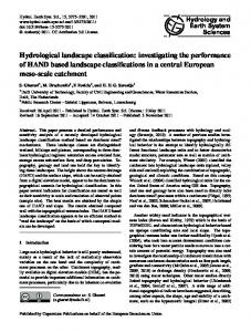
Figure 3: Results of our entire LiDAR classification system using the 3D classifier on (a) D1 and (b) D2. Water points are colored blue, ground points are white, roof points are red, tree points are green, and other points are black.

[2] [3]

[4]

[5]

[6]

[7] [8]

[9]

of markov random fields for segmentation of 3d scan data. IEEE Conf. on Computer Vision and Pattern Recognition 2005, pages 169–176, 2005. 2 L. Breiman. Random forests. Machine Learning, 45:5–32, 2001. 3 J. Caceres and K. Slatton. Improved classification of building infrastructure from airborne lidar data using spin images and fusion with ground-based lidar. Urban Remote Sensing Joint Event, pages 1–7, 2007. 2 A. P. Charaniya, R. M, and S. K. Lodha. Supervised parametric classification of aerial lidar data. IEEE Conf. on Computer Vision and Pattern Recognition Workshop, pages 25– 32, 2004. 2 G. Forlani, C. Nardinocchi, M. Scaioni, and P. Zingaretti. Complete classification of raw lidar data and 3d reconstruction of buildings. Pattern Analysis and Applications, 9(4):357–374, 2006. 2, 7 C. Fr¨uh and A. Zakhor. Constructing 3d city models by merging aerial and ground views. IEEE Comput. Graph. Appl., 23(6):52–61, 2003. 1 R. Gonzalez and R. Woods. Digital image processing, Third Edition. Pearson Prentice Hall, 2008. 7 J.-F. Lalonde, N. Vandapel, D. Huber, and M. Hebert. Natural terrain classification using three-dimensional ladar data for ground robot mobility. Journal of Field Robotics, 23(10):839 – 861, 2006. 2, 4 B. N. Lee. librf: C++ random forests library, 2007. http:

//mtv.ece.ucsb.edu/benlee/librf.html. 7 [10] S. Lodha, D. Fitzpatrick, and D. Helmbold. Aerial lidar data classification using adaboost. Int’l Conf. on 3-D Digital Imaging and Modeling 2007, pages 435–442, 2007. 2 [11] G. Medioni, M.-S. Lee, and C.-K. Tang. A Computational Framework for Segmentation and Grouping. Elsevier Science B.V., 2000. 3 [12] Ohio Wright Center for Data. The wright state 100, 2008. http://www.daytaohio.com/Wright_ State100.php. 2 [13] J. Porway, K. Wang, B. Yao, and S. C. Zhu. A hierarchical and contextual model for aerial image understanding. IEEE Int’l Conf. on Computer Vision and Pattern Recognition, pages 1–8, 2008. 2 [14] J. Secord and A. Zakhor. Tree detection in urban regions using aerial lidar and image data. IEEE Geo. and Remote Sensing Letters, 4(2):196–200, 2007. 2 [15] G. Sithole and G. Vosselman. Experimental comparison of filter algorithms for bare-earth extraction from airborne laser scanning point clouds. ISPRS Journal of Photogrammetry and Remote Sensing, 59(1-2):85–101, 2004. 2 [16] P. Viola and M. Jones. Rapid object detection using a boosted cascade of simple features. IEEE Conf. on Computer Vision and Pattern Recognition, 1:I–511–I–518, 2001. 2 [17] K. Zhang, J. Yan, and S.-C. Chen. Automatic construction of building footprints from airborne lidar data. IEEE Trans. on Geo. and Remote Sensing, 44(9):2523–2533, 2006. 2

[18] P. Zingaretti, E. Frontoni, G. Forlani, and C. Nardinocchi. Automatic extraction of lidar data classification rules. Int’l Conf. on Image Analysis and Processing, 2007, pages 273– 278, 2007. 2