Usability Oriented Visualization Techniques for 3D ... - mediaTUM

Institut für Informatik Technische Universität München

Usability Oriented Visualization Techniques for 3D Navigation Map Display

Mikael Vaaraniemi

Vollständiger Abdruck der von der Fakultät für Informatik der Technischen Universität München zur Erlangung des akademischen Grades eines Doktors der Naturwissenschaften (Dr. rer. nat.) genehmigten Dissertation.

Vorsitzender: Prüfer der Dissertation:

Univ.-Prof. Dr. J. Schlichter 1. Univ.-Prof. Dr. R. Westermann 2. Univ.-Prof. Dr. J. Döllner, Universität Potsdam

Die Dissertation wurde am 19.3.2014 bei der Technischen Universität München eingereicht und durch die Fakultät für Informatik am 21.4.2014 angenommen.

Abstract This thesis presents concepts and techniques that enhance considerably the perception and recognition, visual association, and rendering efficiency of navigation map display. These contributions aim at improving the usability of 3D maps as used in navigation systems and spatial information browsing. The performance of low-end graphical processing units (GPUs) is growing fast [Voi12]: over the next few years, the average GPU performance will increase exponentially and enable high-quality visualization on handheld and embedded devices. At the same time, the market of geographic data is increasing in terms of availability, coverage, precision and semantics. This includes on one hand static data, e.g., freely available and highly detailed vector maps such as OpenStreetMap, which depicts streets, 3D buildings, and land cover usage, and on the other hand dynamic data, e.g., gas prices, local weather, real-time traffic information, or public transportation schedules. In the domain of navigation systems, these trends allow us to present an increasing amount of information and to create high-quality map-based 3D visualization, called in the following “3D maps”. However, the increasing amount of visual information, especially in 3D maps, creates many new problems that hinder usability for navigation systems and spatial information browsing purposes. First of all, the perception and recognition of map elements becomes more difficult, as individual map elements, such as labels or roads, can easily become occluded, e.g., by 3D buildings models. With a freely moving camera, the tracking of labels becomes difficult. Moreover, they can easily overlap each other and hence, become unreadable. Second, it is difficult to maintain a visual association between elements. For example, roads provided as 2D polyline should not disappear below 3D terrain. Labels, floating in the 3D world, should easily be associated to their respective map element, e.g., a road. Finally, 3D buildings and roads created from vector maps should match their respective counterpart in the underlying orthoimage, e.g., an aerial or satellite image. i

ii

In addition to these visual issues, a 3D map decreases the overall system performance as complex textured geometries are drawn, such as 3D buildings and terrain. In the context of navigations systems, maps consist of several semantic layers, e.g., 3D terrain, 3D buildings, roads, labels, and orthoimages. Today’s application and systems typically improve the visualization of a single layer and fail to consider the interdependency between multiple layers; in order to improve the usability in a holistic way, it is essential to consider every layer. Finally, most approaches are designed for powerful desktop GPUs and do not necessarily provide interactive performance on embedded or handheld devices. In this thesis, we propose a set of techniques for rendering 3D maps targeted to enhance the usability of 3D maps for navigation purposes. • First, we will present a technique for rendering cartographic roads with rounded caps on terrain. In its first implementation, a geometric approach enables an efficient rendering of roads onto low to medium-resolution terrain. The second implementation uses shadow-volumes and enables an artifact-free draping of roads on high-resolution terrain. • As second contribution, we introduce a temporal coherent labeling to enable the tracking of labels over the course of navigation. It uses a force-based approach to resolve the collision of labels, while maintaining temporally smooth movements. Additionally, we propose techniques to increase the readability of textual labels and analyze label placement strategies in respect to a 3D geovirtual environment. • The third part of this thesis presents several concepts to enhance the visibility of elements in 3D maps. In a case study, we show how the visibility of labels and roads occluded by 3D buildings can be improved. Two promising approaches were chosen for further evaluation: glowing roads, which allow roads to shine through their occlude, and transparency aura, which creates a transparency region around the label in the occluding object. • The last contribution of this thesis is the procedural generation of orthoimages using real geographic data. A neural network, i.e., a multilayer perceptron, learns automatically the mapping of geographic input to a single color. At runtime, the mapping is evaluated to create a synthetic texture that serves as surrogate for satellite images. Finally, procedural details are added: vegetation is simulated, buildings and fields are procedurally generated and snow is seeded.

iii

All approaches are implemented into a research prototype. We show the performance increase through benchmarks, validate the improved recognition of map elements through user studies and illustrate the enhanced appearance with screenshots. This thesis laid out the foundation for improving 3D maps for navigation systems and applications. Each presented technique can be applied to its respective domain. However, only by enhancing all aspects, specifically the recognition and perception (readability, visibility), visual association (relationship, temporal coherence), and rendering performance, we can significantly improve the display of 3D maps. All in all, the contributions allow the implementation of systems and applications for 3D maps with an improved usability and effectiveness of information display.

Zusammenfassung In dieser Arbeit werden neue Verfahren vorgestellt, um die Erkennung, die bildliche Verbindung und die Darstellungseffizienz von Kartenelementen, bspw. Straßen, Beschriftungen und Satellitenbilder, zu verbessern. Die vorgestellten Verfahren ermöglichen die Verbesserung der Benutzerfreundlichkeit von 3D-Karten zu Navigations- und Informationszwecken. In den nächsten Jahren wird die durchschnittliche Leistung von eingebetteten stromsparenden Grafikkarten (Graphical Processing Units, GPUs) exponentiell wachsen und somit hochwertige Visualisierungen auf tragbaren und eingebetteten Geräten ermöglichen. Zugleich stehen mehr und mehr geografische Daten zur Verfügung: Einerseits statische Daten wie OpenStreetMap, eine frei verfügbare und sehr detaillierte Vektorkarte, die Straßen, 3D-Gebäude und Landnutzungsdaten speichert. Andererseits stehen auch dynamische Daten, bspw. Tankstellenpreise, Wetter oder Verkehrsinformationen zur Verfügung. Im Bereich der Navigationssysteme erlauben uns diese Trends die Präsentation einer zunehmend größeren Menge an Informationen und die Erstellung hochwertiger 3D-Kartenvisualisierungen. Diese zunehmende Menge an dargestellten Informationen bringt jedoch eine Vielzahl neuer Probleme mit sich, welche die Benutzerfreundlichkeit für Navigations- und Informationszwecke erschweren. Zunächst wird die Erkennung von Kartenelementen schwieriger, da einzelne Elemente, wie Beschriftungen oder Straßen, leicht von davorliegenden 3D-Elementen verdeckt werden können, z. B. von 3D-Gebäuden. Zusätzlich gestaltet sich mit einer frei beweglichen Kamera die Verfolgung von Beschriftungen schwierig. Einzelne Schriftzüge können sich leicht überlappen und somit unlesbar werden. Zweitens ist es schwierig, eine bildliche Verbindung zwischen zusammengehörigen Kartenelementen aufrechtzuerhalten. Straßen werden aus einer Vektorkarte als 2D-Linienzug geladen und dargestellt und sollten nicht unter dem 3D-Geländemodell verschwinden. Beschriftungen, die in der virtuellen 3D-Welt platziert werden, sollten v

vi

ihrem jeweiligen Kartenelement einfach zugeordnet werden, bspw. ihrer zugehörigen Straße. Schließlich sollten aus Vektorkarten gewonnene 3D-Gebäude und Straßen mit ihrem jeweiligen Pendant in dem darunterliegenden Orthofoto, bspw. einer Luft- oder Satellitenaufnahme, übereinstimmen. Neben diesen visuellen Themen stellt eine 3DKartendarstellung neue Herausforderungen an die Leistung eines Systems, unter anderem bei der Anzeige von 3D-Gebäuden und eines hoch aufgelösten Geländemodells. Thematische Karten bestehen aus mehreren semantischen Schichten, z.B. Orthofotos, 3D-Geländemodellen, Straßen, 3D-Gebäuden und Beschriftungen. In aller Regel betrachten bestehende Verfahren nur eine einzige solche Schicht. Es ist jedoch essentiell, jede sichtbare Schicht zu behandeln, um die Benutzerfreundlichkeit in Ihrer Gesamtheit zu verbessern. Des Weiteren sind die meisten bestehenden Ansätze nur für leistungsstarke GPUs entwickelt worden und in aller Regel ungeeignet für stromsparende eingebettete Systeme. In dieser Arbeit werden mehrere Ansätze vorgestellt, um die Benutzerfreundlichkeit von 3D-Karten zu Navigations- und Informationszwecken zu verbessern. • Im ersten Teil dieser Arbeit werden zwei Verfahren zur Abbildung von kartographischen Straßen mit abgerundeten Kappen auf 3D-Geländemodellen beschrieben. Der erste Ansatz, der geometrische Ansatz, ermöglicht eine effiziente Darstellung von Straßen auf Geländemodellen mit niedriger bis mittlerer Auflösung. Der zweite Ansatz, der Shadow-Volume Ansatz, ermöglicht eine fehlerfreie Abbildung von Straßen auf hochauflösenden Geländemodellen. • Im zweiten Teil dieser Arbeit werden Verfahren zur Ermöglichung einer zeitlich kohärenten Beschriftung von 3D-Karten vorgestellt. Dies erlaubt die Verfolgung von Beschriftungen während einer Navigation, bspw. wenn die virtuelle Kamera die aktuell geplante Route verfolgt. Das in dieser Arbeit vorgestellte Verfahren nutzt einen kräftebasierten Ansatz, um auftretende Kollisionen zwischen Beschriftungen sanft aufzulösen. Außerdem werden Techniken vorgeschlagen um die Lesbarkeit von Textbeschriftungen zu steigern. Schließlich werden mögliche Strategien zur Beschriftungsplatzierung in virtuellen 3D-Welten analysiert. • Der dritte Teil dieser Arbeit stellt Konzepte vor, um die Sichtbarkeit von verdeckten Elementen in 3D-Karten zu erhöhen. Als Fallstudie wird die Sichtbarkeit von Beschriftungen und Straßen, die von 3D-Gebäuden verdeckt wurden, verbessert. Zwei vielversprechende Ansätze wurden zur weiteren Auswertung gewählt: das

vii

erstes Konzept, leuchtende Straßen, deutet Straßen durch das davorliegende Objekt an. Das zweite Konzept, die transparente Aura, erschafft eine transparente Fläche im davorliegenden Objekt, um die Beschriftungen erscheinen zu lassen. • Der letzte Teil dieser Arbeit präsentiert ein Verfahren zur prozeduralen Generierung von Orthofotos mit Hilfe realer geografischer Daten. Ein neuronales Netz, ein mehrschichtiges Perzeptron, lernt automatisch die Zuordnung von geographischen Eingangsdaten zu einer Ausgangsfarbe. Zur Laufzeit wird diese Zuordnung ausgewertet, um eine synthetische Textur zu erstellen. Schließlich werden prozedurale Details hinzugefügt: es wird Vegetation simuliert, Gebäude und Felder werden prozedural erstellt und Schnee wird auf Bergen gesät. Das entstandene künstliche Bild kann stellvertretend für eine Satelliten- oder Luftaufnahme verwendet werden. Alle präsentierten Verfahren wurden in einem Forschungsprototyp implementiert. Die Leistungssteigerung werden durch Messungen gezeigt, die verbesserte Erkennung von Kartenelementen durch Nutzerstudien bestätigt und die qualitativ verbesserte Darstellung durch Screenshots belegt. In dieser Arbeit wird der Grundstein zur Verbesserung der Benutzerfreundlichkeit von 3D-Karten zu Navigations- und Informationszwecken gelegt. Jedes vorgestellte Verfahren kann in seinem respektiven Anwendungsbereich eingesetzt werden. Jedoch führt nur die Verbesserung mehrerer Schlüsselaspekte, insbesondere der Erkennung (Lesbarkeit, Sichtbarkeit), der bildlichen Verbindung (Beziehung, zeitliche Kohärenz) und der Darstellungseffizienz, zu einer deutlichen Verbesserung der Darstellung von 3DKarten. Die Kombination der vorgestellten Verfahren ermöglicht die Entwicklung von Systemen und Anwendungen für 3D-Karten mit einer deutlich verbesserten Benutzerfreundlichkeit und Effektivität der Informationsdarstellung.

Acknowledgments I am most grateful to my Ph.D. supervisor, Rüdiger Westermann, for actively supervising my thesis all these years with his constructive feedback and interesting discussions. Thank you for giving me the possibility to do research in this area. Moreover, your support enabled me to attend international conferences, which gave me insight into the many facets of the scientific community. I am very thankful to my second Ph.D. supervisor, Jürgen Döllner, for the active feedback and all the constructive and fresh ideas from a cartographic and GIS point-of-view. I am most thankful to my direct superior, Robert Hein, for his long patience and for giving me the opportunity and enough freedom to write my Ph.D. thesis in his group at BMW Research. This would not have been possible without your support. I would like to express my gratitude to Philipp Promesberger for the implementation of the map viewer framework and for all the long discussions, criticism and tips throughout the thesis. Many thanks to my fellow colleagues, Klaas Klasing and Andreas Hackelöer, for their very contructives reviews and advices. Moreover, I am most grateful to all fellow friends who pursued or are still pursuing their own Ph.D., Roland Bader, Thomas Mangel, Max Graf, Benno Schweiger, Olga Birth and Alexandre Bouard. They gave me all the support, criticism and pushes I needed to finish this thesis. Thanks to all my former or current colleagues: Christian Spies, Michael Karg, Klaus Goffart, Markus Strassberger, Axel Jansen, Dominik Gusenbauer, Isabella Szottka, Hendrik Schweppe, Martin Schäfer, Lutz Ehnert, Andrea Binter and Daniel Niehues. I am grateful for the continuous feedback from Christopher Roelle from our user experience team while designing the labeling techniques. I would also like to thank all my former students: Michael Genau for the first force-based labeling approach, Tim Oppermann for the first synthetic orthoimages, Johannes Treitz for textured overlays on DTMs, and Matthias Winkler for implementing the first prototype for label filtering. Many thanks to my student and co-author Martin Freidank for the hard work on the 3D city labels paper. I would like to thank Marco Matt for preparing and conducting ix

x

the expert and user studies at our research labs. I am very grateful to my co-authors, Aick in der Au and Florian Jarmer, for their respective work on the implementation of the synthetic orthoimages and the first essay on a scientific publication. Moreover, my thank goes to Alexander Mellich and Heiko Achilles for their design lead and creating the orthoimage texture atlas. A big thank you to my co-author, Marc Treib, for all the excellent input, reviews, and support he gave me throughout this thesis. The short trip with him to the WSCG conference in Plzeˆn will be remembered. I would also like to thank Christian Dick, Kai Bürger, Shuntin Cao, Stefan Auer and Roland Fraedrich from the Technische Universität München for all the long and interesting discussions we had during coffee breaks. Many thanks to Tobias Schafhitzel, Ralf Botchen and Martin Falk from the University of Stuttgart for giving me a first insight into scientific work and starting my idea to pursue a Ph.D. thesis. A warm and whole-hearted thank you to Evamaria Prager for just being there for me. It goes without saying that I am most thankful to my father, mother, and sister for the best support of all.

Contents Abstract

i

Zusammenfassung

v

Acknowledgments

ix

1

Introduction 1.1 Problems . . . . . . . . . . . . . . . . . . . . . . . . . . . . . . . . . 1.2 Contributions . . . . . . . . . . . . . . . . . . . . . . . . . . . . . . . 1.3 Publications . . . . . . . . . . . . . . . . . . . . . . . . . . . . . . . .

1 2 3 5

2

Fundamentals 2.1 Geographic Information Systems . . . . . . . . . . . . . . . . . . 2.1.1 Geographical Object . . . . . . . . . . . . . . . . . . . . 2.1.2 Data Models . . . . . . . . . . . . . . . . . . . . . . . . 2.1.3 OpenStreetMap . . . . . . . . . . . . . . . . . . . . . . . 2.1.4 Web Services for Geodata . . . . . . . . . . . . . . . . . 2.2 Real-Time Rendering . . . . . . . . . . . . . . . . . . . . . . . . 2.2.1 Rendering Pipeline . . . . . . . . . . . . . . . . . . . . . 2.2.2 The OpenGL API . . . . . . . . . . . . . . . . . . . . . . 2.3 Evolution of Map Visualization . . . . . . . . . . . . . . . . . . . 2.3.1 3D Map Viewers for Virtual Globes . . . . . . . . . . . . 2.3.2 Map Viewers for Digital Automotive Navigation Systems 2.3.3 Cartographic Map Visualization Techniques . . . . . . . .

3

. . . . . . . . . . . .

. . . . . . . . . . . .

. . . . . . . . . . . .

7 7 7 8 11 11 13 16 18 20 20 22 26

High-Quality Cartographic Roads on High-Resolution DEMs 27 3.1 Introduction . . . . . . . . . . . . . . . . . . . . . . . . . . . . . . . . 28 3.2 Related Work . . . . . . . . . . . . . . . . . . . . . . . . . . . . . . . 29 xi

xii

CONTENTS

3.3 3.4 3.5

3.6

3.7 3.8 4

Cartographic Roads . . . . . . . Geometric Approach . . . . . . Shadow Volume Approach . . . 3.5.1 Intersection . . . . . . . 3.5.2 Numerical Precision . . Implementation Details . . . . . 3.6.1 Geometry Clipping . . . 3.6.2 Geometry Z-Offset . . . 3.6.3 Cartographic Rendering Results . . . . . . . . . . . . . . Conclusions . . . . . . . . . . .

. . . . . . . . . . .

. . . . . . . . . . .

. . . . . . . . . . .

. . . . . . . . . . .

. . . . . . . . . . .

. . . . . . . . . . .

. . . . . . . . . . .

. . . . . . . . . . .

. . . . . . . . . . .

. . . . . . . . . . .

. . . . . . . . . . .

. . . . . . . . . . .

. . . . . . . . . . .

. . . . . . . . . . .

Temporally Coherent Real-Time Labeling of Dynamic Scenes 4.1 Introduction . . . . . . . . . . . . . . . . . . . . . . . . . 4.2 Related Work . . . . . . . . . . . . . . . . . . . . . . . . 4.3 Preliminary Study . . . . . . . . . . . . . . . . . . . . . . 4.3.1 Study Design . . . . . . . . . . . . . . . . . . . . 4.3.2 Results . . . . . . . . . . . . . . . . . . . . . . . 4.3.3 Design Principles . . . . . . . . . . . . . . . . . . 4.4 Force-Based Labeling . . . . . . . . . . . . . . . . . . . . 4.4.1 Motivation . . . . . . . . . . . . . . . . . . . . . 4.4.2 Features . . . . . . . . . . . . . . . . . . . . . . . 4.4.3 Initial Placement . . . . . . . . . . . . . . . . . . 4.4.4 Collision . . . . . . . . . . . . . . . . . . . . . . 4.4.5 Forces and Movement . . . . . . . . . . . . . . . 4.4.6 Acceleration . . . . . . . . . . . . . . . . . . . . 4.5 Implementation . . . . . . . . . . . . . . . . . . . . . . . 4.5.1 Parallelization . . . . . . . . . . . . . . . . . . . 4.5.2 Rendering Textual Annotations . . . . . . . . . . 4.5.3 Enhancements . . . . . . . . . . . . . . . . . . . 4.6 Results . . . . . . . . . . . . . . . . . . . . . . . . . . . . 4.6.1 Scalability . . . . . . . . . . . . . . . . . . . . . 4.6.2 Concluding Expert Study . . . . . . . . . . . . . . 4.6.3 Cartographic Principles . . . . . . . . . . . . . . . 4.7 Conclusions . . . . . . . . . . . . . . . . . . . . . . . . .

. . . . . . . . . . .

. . . . . . . . . . . . . . . . . . . . . .

. . . . . . . . . . .

. . . . . . . . . . . . . . . . . . . . . .

. . . . . . . . . . .

. . . . . . . . . . . . . . . . . . . . . .

. . . . . . . . . . .

. . . . . . . . . . . . . . . . . . . . . .

. . . . . . . . . . .

. . . . . . . . . . . . . . . . . . . . . .

. . . . . . . . . . .

. . . . . . . . . . . . . . . . . . . . . .

. . . . . . . . . . .

31 33 34 35 36 37 37 38 38 40 43

. . . . . . . . . . . . . . . . . . . . . .

45 46 47 50 50 50 51 52 52 53 54 54 57 59 59 59 60 61 62 62 63 65 66

CONTENTS

xiii

5

. . . . . . . . . . . . . . . . . . . . . .

67 68 69 69 69 70 71 71 71 72 73 73 74 74 74 76 76 77 77 78 78 81 84

. . . . . . . . . . .

85 86 87 89 90 92 94 96 97 99 101 101

6

Enhancing the Visibility of Labels in 3D Navigation Maps 5.1 Introduction . . . . . . . . . . . . . . . . . . . . . . . 5.2 Labeling Techniques . . . . . . . . . . . . . . . . . . 5.2.1 World-Space and Screen-Space Labels . . . . . 5.2.2 External and Internal Labels in 3D Worlds . . . 5.2.3 Summary . . . . . . . . . . . . . . . . . . . . 5.3 Concepts . . . . . . . . . . . . . . . . . . . . . . . . 5.3.1 Baseline . . . . . . . . . . . . . . . . . . . . . 5.3.2 Cutaways . . . . . . . . . . . . . . . . . . . . 5.3.3 Transparency Label Aura . . . . . . . . . . . . 5.3.4 Glowing Labels . . . . . . . . . . . . . . . . . 5.3.5 Glowing Roads . . . . . . . . . . . . . . . . . 5.4 Expert Study . . . . . . . . . . . . . . . . . . . . . . 5.4.1 Study design . . . . . . . . . . . . . . . . . . 5.4.2 Discussion . . . . . . . . . . . . . . . . . . . 5.4.3 Results . . . . . . . . . . . . . . . . . . . . . 5.5 Implementation . . . . . . . . . . . . . . . . . . . . . 5.5.1 Transparency Label Aura . . . . . . . . . . . . 5.5.2 Glowing Streets . . . . . . . . . . . . . . . . . 5.6 Results . . . . . . . . . . . . . . . . . . . . . . . . . . 5.6.1 Benchmark . . . . . . . . . . . . . . . . . . . 5.6.2 User Study . . . . . . . . . . . . . . . . . . . 5.7 Conclusions . . . . . . . . . . . . . . . . . . . . . . .

. . . . . . . . . . . . . . . . . . . . . .

. . . . . . . . . . . . . . . . . . . . . .

. . . . . . . . . . . . . . . . . . . . . .

. . . . . . . . . . . . . . . . . . . . . .

. . . . . . . . . . . . . . . . . . . . . .

. . . . . . . . . . . . . . . . . . . . . .

Procedural Generation of Orthoimages with Real Geographic Data 6.1 Introduction . . . . . . . . . . . . . . . . . . . . . . . . . . . . . 6.2 Related Work . . . . . . . . . . . . . . . . . . . . . . . . . . . . 6.3 Overview . . . . . . . . . . . . . . . . . . . . . . . . . . . . . . 6.3.1 System . . . . . . . . . . . . . . . . . . . . . . . . . . . 6.4 Geographic Data Sources . . . . . . . . . . . . . . . . . . . . . . 6.5 Pre-processing of Geographic Data . . . . . . . . . . . . . . . . 6.6 Generation of Synthetic Orthoimages . . . . . . . . . . . . . . . 6.6.1 Neural Network Architecture and Training . . . . . . . . 6.6.2 Neural Network Execution on the GPU . . . . . . . . . . 6.7 Detail Generation . . . . . . . . . . . . . . . . . . . . . . . . . . 6.7.1 Vegetation Simulation . . . . . . . . . . . . . . . . . . .

. . . . . . . . . . . . . . . . . . . . . .

. . . . . . . . . . .

. . . . . . . . . . . . . . . . . . . . . .

. . . . . . . . . . .

xiv

CONTENTS

. . . . . . . . .

102 105 106 106 107 107 107 108 112

Summary, Conclusions, and Outlook 7.1 Summary . . . . . . . . . . . . . . . . . . . . . . . . . . . . . . . . . 7.2 Discussion . . . . . . . . . . . . . . . . . . . . . . . . . . . . . . . . . 7.3 Future Work . . . . . . . . . . . . . . . . . . . . . . . . . . . . . . . .

115 115 116 119

6.8

6.9 7

6.7.2 Field Generation 6.7.3 Urban Rendering 6.7.4 Relief shading . 6.7.5 Multi-Resolution 6.7.6 Editor . . . . . . Results . . . . . . . . . . 6.8.1 Comparison . . . 6.8.2 Benchmark . . . Conclusions . . . . . . .

Bibliography

. . . . . . . . .

. . . . . . . . .

. . . . . . . . .

. . . . . . . . .

. . . . . . . . .

. . . . . . . . .

. . . . . . . . .

. . . . . . . . .

. . . . . . . . .

. . . . . . . . .

. . . . . . . . .

. . . . . . . . .

. . . . . . . . .

. . . . . . . . .

. . . . . . . . .

. . . . . . . . .

. . . . . . . . .

. . . . . . . . .

. . . . . . . . .

. . . . . . . . .

. . . . . . . . .

. . . . . . . . .

. . . . . . . . .

. . . . . . . . .

125

Chapter 1

Introduction Navigation systems have become ubiquitous in recent years. Integrated into a multitude of devices, they can be found in portable devices, cars, smartphones, tablets, and even virtual reality glasses, such as Google Glasses. They help the user to navigate in and to unknown destinations by different means, including planning a route to a destination (route planning), computing the current location (positioning), guiding through voice (guidance) and showing a map of the environment (map viewer). The main task of a map viewer is the visual representation of internal navigation states: the current position, the planned route and guidance hints. Moreover, displaying a map enhances the user’s relative spatial orientation: Where is his/her location in respect to other streets, cities and important locations? As increasingly more geographic data become freely available, we can enrich such maps with more visual information. For instance, OpenStreetMap [Ope] provides us world-wide vector data for rendering roads, building footprints and Points-of-Interest. CORINE [Eur00] gives us land-cover data and SRTM [FRCCD+07] provides 3D terrain information. Furthermore, we can add dynamic data such as gas prices, weather, real-time traffic information, and public transportation schedules. This leads us to the second task of a map viewer, popularized for example by Google Maps, namely spatial information browsing. For this task, a plethora of choices is currently available, ranging from Bing Maps, Apple’s iOS Maps and Nokia Maps to virtual earth explorers like Google Earth (Chapter 2.3). Integrated into smartphones, these browsers allow location-based services to display their respective dynamic data. For instance, Yelp and Foursquare present restaurant and bar recommendations, while Waze displays its community created map. In parallel, the performance of graphical processing units (GPUs) in systems on a chip (SoC) is rising exponentially, e.g., with the Nvidia Tegra SoCs and PowerVR 1

2

CHAPTER 1. INTRODUCTION

SGX GPUs. Furthermore, the latest iterations of computer graphics standards, such as OpenGL ES 3.0, introduce advanced features to the embedded world, including depth and floating point textures, multiple render targets, and full-precision shader operations [Lip13]. With these developments, computer graphics on embedded devices will leap, in the coming years, from simple shaded graphics using a fixed-function pipeline to fully-fledged, shader-powered engines. At first glance, this trend allows us to create advanced map representations, enhancing the overall appearance with a higher screen resolution, more details and better lighting models to create a photorealistic or highquality non-photorealistic rendering (NPR). Moreover, with the increased processing power, we can jump from a 2D to 3D map representation, namely a virtual globe with a digital elevation model (DEM) and 3D buildings to create a more faithful representation of the world. This allows users to recognize objects from the real world more easily in the digital map. Therefore, it augments their ability for spatial orientation and they can map the navigation guidance to the surrounding world. Such state-of-the-art 3D maps are present in current portable navigation software (e.g., Sanyo, Apple, Garmin, Navigon, Bosch and Falk) and automotive navigation systems (e.g., Audi, BMW).

1.1

Problems

However, the increasing amount of visual information, especially represented in a 3D map, creates many new problems, hindering usability for navigation and spatial information browsing purposes. In 3D maps, the perception and recognition (or readability) of information is difficult to design and guarantee compared to their 2D counterparts. The inherent perspective transformation creates conflicting goals: it helps spatial orientation yet hinders the recognition of elements, given that they get smaller when they are further away. Furthermore, as occlusion occurs, the visibility of objects is hindered, e.g., when buildings hide labels and roads. As the camera moves freely, collisions between labels are frequent and cannot be avoided with pre-computation, as it is usually done for 2D maps. Finally, both occlusion and 3D movement make the tracking of map elements more difficult. This increases the amount of time in which an element, e.g., a label, can be recognized and read. After recognition, the second most important aspect relates to the visual association of an element to its feature. Labels should be easy to associate with their corresponding features, e.g., a road. Moreover, roads, land-cover and 3D buildings from vector maps should match their respective counterparts in the underlying orthoimage. Finally, roads

1.2. CONTRIBUTIONS

3

should match the DEM to avoid them disappearing in mountains or floating in the air. All current navigation systems and GIS, e.g., Google Earth, exhibit problems in resolving these aforementioned issues. With increasingly more information to be processed, 3D maps require an efficient rendering of elements. In large cities, such as Tokyo or London, it is necessary to render complex road networks together with thousands of buildings, while also placing hundreds of annotations in real-time. Finally, we want high-quality rendering of DEM and 3D cities with features such as anti-aliasing and ambient occlusion; however, creating such a rendering represents an even greater challenge on embedded hardware. While current systems use Level-of-Detail approaches, smaller viewing frustums and additional fog to reduce the performance hit, these techniques impede our primary goals, namely the visibility and recognition of map elements.

1.2

Contributions

To tackle the aforementioned problems, we propose a set of techniques, each of which solves distinct weaknesses of current map viewers in order to increase the overall usability of 3D maps. In Chapter 3, we introduce the cartographic rendering of roads onto terrain. Similar to paper maps, such rendering creates a clear and uncluttered representation to allow a quick recognition of roads and their properties; it requires runtime scaling of the road’s width, dark outlines, vivid colors and rounded caps at both ends. Accordingly, we will present two high-performance GPU-based solutions fulfilling these requirements. The first implementation enables an efficient rendering of roads with a geometric approach. The road from a vector database is sent as polyline to the GPU and inflated to rectangles in the geometry shader. Subsequently, based on the resulting rectangles, the rounded caps are evaluated analytically in the fragment shader. The second implementation extends the shadow-volume algorithm to project roads with rounded caps. First, we extrude the polyline of the road along the nadir. Then, we generate a stencil mask by computing the screen-space intersection between the created polyhedra and the terrain geometry. With this mask, we render single colored fullscreen rectangles for every road class. This method is independent of the terrain rendering algorithm and creates a per-pixel exact and artifact-free projection onto any DEM. We perform benchmarks, determining that our geometric approach works best on low- to medium-resolution terrain, while the shadow-volume approach scales best on high-resolution terrain. Finally,

4


we depict the resulting image quality improvements with screenshots. In Chapter 4, we introduce a temporally coherent labeling approach, which computes an annotation layout in real-time and resolves collisions between labels using a force-based approach. This solution creates temporally smooth movements and enables an easy tracking of labels over the course of a navigation, i.e., when the camera follows the currently planned route. Forces allow the flexible definition of runtime behaviors, whereby labels can move freely (e.g., POIs), circle around their point feature (e.g., cities) or slide along their line feature (e.g., roads). Additionally, we propose techniques to fulfill the cartographic principles defined by Imhof [Imh75], which include readability, visual association and classification. Finally, two benchmarks show how the GPU-based implementation can create layouts for several thousand labels in real-time. An expert study confirms the enhancements achieved by our algorithm with respect to visual association and readability. In Chapter 5, we introduce several concepts to enhance the visibility of occluded elements in 3D maps. As a case study, we improve the visibility of labels and roads occluded by 3D buildings. The conducted expert study establishes two concepts for further evaluation, chose predominantly because they retain a visual association to the related object, e.g., the label to the road. The first method, called glowing roads, lets roads shine through their occlude, whereas the second method, called transparency aura, creates a transparency region around the label in the occluding object. For both methods, we present a GPU-based implementation. A concluding user study validates the usability improvement, with both approaches performing significantly better compared to our baseline of simply drawing labels over occluding objects. Indeed, they acquire the focus of the user (recognition) while keeping the context intact (visual association). In Chapter 6, we introduce the procedural generation of orthoimages using real geographic data. In a pre-processing step, a neural network, i.e., a multilayer perceptron, learns the mapping of geographic input to a single color from a real satellite image. At runtime, the mapping is evaluated for every pixel to create a surrogate of an orthoimage. Because the geographic input has a limited resolution, procedural details are added, with vegetation simulated, crops procedurally generated, and snow seeded on mountain tops. Finally, roads and buildings from a vector database are rendered on top. We compare the resulting images with real orthoimages, i.e., satellite images. The procedural images are free of occluding artifacts, e.g., clouds and shadows. Moreover, they have a coherent coloration and do not exhibit tiling problems. Finally, they match all overlaid renderings created with the same vector database, e.g., cartographic roads,

1.3. PUBLICATIONS

5

3D buildings and land-cover areas. We conclude this thesis in Chapter 7 with a brief summary of all contributions, before presenting a juxtaposition of all aspects covered by this thesis. We classify the improvements into separate domains: recognition (e.g., enhanced readability and visibility), visual association (e.g., better matching and relationship), temporal coherence (e.g., enhanced tracking) and rendering efficiency. Finally, we show promising directions for future research work.

1.3

Publications

This thesis is partly based on the following peer-reviewed research papers (listed in chronological order): • Lothar Stolz, Holger Endt, Mikael Vaaraniemi, Daniel Zehe, and Walter Stechele. “Energy consumption of Graphic Processing Units with respect to automotive use-cases”. In: Proceedings of the International Conference on Energy Aware Computing. ICEAC. IEEE. 2010, pp. 1–4. ISBN: 978-1-4244-8273-3 [SEVZS10] • Mikael Vaaraniemi, Marc Treib, and Rüdiger Westermann. “High-Quality Cartographic Roads on High-Resolution DEMs”. In: Journal of WSCG 19.2 (2011), pp. 41–48. ISSN: 1213-6972 [VTW11] • Mikael Vaaraniemi, Marc Treib, and Rüdiger Westermann. “Temporally Coherent Real-Time Labeling of Dynamic Scenes”. In: Proceedings of the 3rd International Conference on Computing for Geospatial Research and Applications. COM.Geo ’12. ACM, 2012, 17:1–17:10. ISBN: 978-1-4503-1113-7. DOI: 10.1145/2345316.2345337 [VTW12] • Mikael Vaaraniemi, Martin Freidank, and Rüdiger Westermann. “Enhancing the Visibility of Labels in 3D Navigation Maps”. In: Progress and New Trends in 3D Geoinformation Sciences. Lecture Notes in Geoinformation and Cartography. Springer, 2012, pp. 23–40. ISBN: 978-3-642-29792-2. DOI: 10.1007/9783-642-29793-9_2 [VFW12]

6


Chapter 2

Fundamentals 2.1

Geographic Information Systems

A geographic information system (GIS) is a location-based information system modeling the real world. It digitally captures, stores, manages, analyzes and presents locationbased datasets as alpha-numerical or graphical output [Lan06, Chapter 9]. Relating objects to a geographical position within a reference system creates a geographical object. Usually, we use geographical coordinates, i.e., latitude and longitude, to specify its position on the surface of the earth. “A GIS is a computer-based system to aid in the collection, maintenance, storage, analysis, output, and distribution of spatial data and information” [Bol07, Chapter 1] 2.1.1

Geographical Object

A geographic object is the fundamental unit of a GIS. It represents a unique entity of the earth which is physically, geometrically or thematically limited [RJK03]. Norbert de Lange defines geographical objects as follow: Geographical objects are spacial elements which exhibit geometrical, topological and temporal properties in addition to their semantic information [Lan06, p. 181]. As such, geographic objects are an abstraction of reality. The produced representation of the real world is a digital model with a defined precision. Geographical objects can be classified into points, lines, and areas features, and solid figures [Imh75]. For example, point features can define border stones or Points-of-Interest, line features can represent water pipelines or roads, area features displays municipal areas or land-cover and solid figures represent 3D buildings or trees. This feature-based classification defines one 7

8

CHAPTER 2. FUNDAMENTALS

possible organization of geographic data (refer to thematic layers in Section 2.1.2). Another approach consists in an object-oriented model, i.e., general objects can be derived into specialized objects. A child object (e.g., a motorway) would inherit its attributes from a base object (e.g., a road) [Lan06, p.160]. For managing, processing and visualizing these objects we must create appropriate structures, called data models. 2.1.2

Data Models

A data model is the abstraction, representation and organization of real-world elements [Kap01]. Therein, the geometry, topology, semantic and relationship of real objects has to be abstracted enough to generate a corresponding data model representation [Ble 0]. This allows us to map reality to data structures for computational and visualization purposes in a GIS. On a higher level, we organize geographical objects using two fundamental principles: within a layer or within an object-oriented model. On a lower level, we differentiate between a raster-based and vector-based model. Thematic Layer Concept

The thematic layer concept originates from cartography, where mapmakers created transparencies that could be overlaid on a light table. Hence, by combining different layers, they could create their desired information density in an analog map. This concept represents the default form of data organization within a GIS. It follows a topdown approach to create a thematic sorting of all geographic input information. Each layer represents a distinct data theme consisting of a collection of common geographic elements, e.g., a road network, a digital elevation model or urban areas (Fig. 2.1). Thematic layers have several key advantages. First, they represent an intuitive way to organize and view data in a GIS. Second, errors occurring in a layer only have a local impact. Finally, they are efficient resource-wise, because only requested layers are processed and visualized.

Vector, Raster and Hybrid Data Models

The thematic layer concept creates a high-level organization of data. However, we need lower-level models to organize data within a layer, e.g., how to store and organize the data of the road network layer. These are called geometrical-topological data models.

2.1. GEOGRAPHIC INFORMATION SYSTEMS

9

Figure 2.1: Thematic Layers organize the geographical data into distinct themes. In this image, Points-of-Interest, orthoimages, elevation data and water bodies represent distinct layers.

The following section describes two fundamental models: the vector data model and the field-based raster data model. Vector Data Model. Vector data models represent information as points, lines and polygons (see [Bar05] and Fig. 2.2). In a GIS, the OGC and ISO committees define these basic geometrical elements as Simple Features (see ISO 19125 [Iso]). This model discretizes the geometry of real world elements. All geographic elements of the vector data model are based on point coordinates, e.g., latitude and longitude. The topological relationship is stored explicitly [Lan06], e.g., which points create a line or an area. Using further attributes, we define the thematic relationship, e.g., whether a line is a road. Therefore, the vector data model is also called the georelational data model (see [Bar05, p.64]).

Figure 2.2: Basic elements from the vector data model called Simple Features [Iso]: (left) Point features, e.g., Point-of-Interest. (middle) Line features, e.g., roads. (right) Polygon features, e.g., land-cover.

This model presents several advantages (see [Buc97]). Geographical data can be represented with its originally captured resolution. In a cartographic representation, the graphical output is usually more aesthetically pleasing. Also, simple geometrical elements can usually be very efficiently encoded into vector data, e.g., a road network. Topology is easily stored and enables efficient topological operations, e.g., network analysis. However, continuous data, e.g., temperature or elevation data, is not effectively stored in vector form. Furthermore, the complexity of data operations is proportional to the number of simple features present.

10


Field-based Data Model. The field-based model partitions the theme of the geographic input surface into homogeneous areas (cells). The form and size of these cells can be defined freely. However, as a whole, they should cover the entire input surface (see [Bar05, p.62ff]). Therefore, each cell explicitly stores georeferenced thematic information (Fig. 2.3). An example for the field-based concept is the DEM, wherein each cell represents the averaged height inside the covered input surface.

Thematic Information

Input Surface

Figure 2.3: The field-based data model (based on [Bar05]) partitions the input space into homogeneous cells, e.g., pixels. Each cell stores thematic information, e.g., its averaged altitude.

Raster Data Model. In GIS, the raster data model is used to represent continuous data over space. It is a specialization of the field-based model. The input surface is divided into equally sized areas, usually a quadratic cell, i.e., pixel. For example, every cell stores the ambient temperature or the averaged height. The size of the cells defines the perceivable data resolution (see [Bar05, p.64f]). The raster data model has several advantages (see [Buc97]). In comparison to the vector model, the geographic coordinates are not explicitly stored. If the geographic location and extend of the entire grid is defined, the position of every pixel is implicit in the layout of the grid. Moreover, the theme (e.g., the temperature) is given implicitly and not explicitly like in the vector model. Hence, data processing and analysis is usually quite simple to perform. It is perfectly suited for continuous data. However, the cell size determines the resolution for processing and visualizing the data. Hence, it is difficult to adequately represent linear geographical elements, i.e., simple features. Usually, storing this data at a high precision comes at the expense of a very high storage cost.

2.1. GEOGRAPHIC INFORMATION SYSTEMS

11

Summary

The vector data model is based on basic elements. This makes it very efficient storagewise. For example, a line is stored as start and end point. All points in-between are defined implicitly by its topology. However, the geographic surface is usually not covered completely. But we can define very precisely the form and position of geographical objects. The main disadvantage of the raster model is the deformation of the geometrical input involved in the storage into a grid. For example, curves can become heavily aliased (jagged, staircase effect). Increasing the resolution diminishes this unwanted effect. However, this involves higher storage costs. Another advantage of the vector model is the simple coordinate transformation. In comparison, the raster model makes it easy to find neighbors and to apply image-based algorithms (see [Bar05, p.68f]). Finally, the raster model has a very simple and distinct element: a pixel. 2.1.3

OpenStreetMap

The OpenStreetMap project started in 2004 and is a prime example of Volunteered Geographic Information (VGI). It is a collaborative project that aims to create a freely available digital map of the whole world [Ope]. The map is either hand-drawn in graphical editors or generated from sensed geographic data, e.g. GPS traces from portable navigation devices. The vector-based OpenStreetMap data model is derived from GDF. The amount and quality of the digitized geographic data are steadily increasing, to the extent that the map is now widely recognized as being comparable in quality to commercial providers [NZZ11], e.g., Nokia and TomTom. Active regions such as urban areas often exhibit a higher level of detail than commercial alternatives. In contrast, rural and poorer areas lack coverage [Hak10]. However, similar to Wikipedia, the quality of the collaborative map depends on the corrections provided by the community. Nevertheless, OpenStreetMap is used in many open-source and commercial products, e.g., Apple Maps, Wikipedia, Foursquare, Skobbler Navigation or Flickr. 2.1.4

Web Services for Geodata

In the last decade, the Open Geospatial Consortium (OGC) standardized several web services for accessing and visualizing geographic data. Web Map Service (WMS) [LB06] is a protocol for serving georeferenced 2D map images over the Internet. For each WMS request, the server generates single static images from a GIS database for a spatial region in the form of PNG, GIF or JPEG images. In 2010, the OGC published the Web Map Tile Service (WMTS) [JMJ10] protocol that serves predefined

12


(a)

(b)

(c)

(d)

Figure 2.4: Comparison of OpenStreetMap (a) and web-based viewers using commercial map data: (b) Bing Maps, (c) Yahoo Maps and (d) Google Maps.

georeferenced 2D map tiles. In contrast to WMS, the client of a WMTS stitches the tiles to a seamless 2D map. This allows the server to pre-render and cache the tiles, hence increasing the performance when handling simultaneous requests. As a semantic counterpart to WMS, the Web Feature Service (WFS) [Vre05] allows querying and retrieving the definition of geographic objects inside the requested bounding region. Moreover, the WFS-T standard defines transaction requests to allow the creation, deletion and update of geographic features stored on a server. Currently, the transmission and display of 3D scenes over web-based services is an ongoing effort. Two alternatives are currently reviewed by the OGC to create a common base for service interfaces: The OGC draft of the Web 3D Service (W3DS) [AS10] defines a protocol to stream 3D scenes, such as textured 3D geometry, to its clients. The rendering of these 3D scenes is done on the client side. In contrast, the Web View Service (WVS) [Hag10] renders images of 3D geovirtual environments on the server side. This allows thin clients, i.e., smartphones and tables, to display rich 3D environments, e.g., virtual 3D city models [JK13].

2.2. REAL-TIME RENDERING

2.2

13

Real-Time Rendering

Rendering virtual 3D environments such as a geovirtual world of a GIS is a challenging task. We have to define a virtual camera, light sources, and place geographic objects into a virtual 3D scene. These scenes are usually defined with geometrical primitives, i.e., lines, triangles, and polygons. Various techniques exist to generate 2D raster image representations out of such 3D scenes. Prominent approaches are ray tracing and rasterization. Currently, interactive computer graphics can be achieved for both approaches. However, only rasterization can be easily computed by commodity GPU hardware. This enables 3D map visualizations on desktop PCs and embedded SoCs, e.g., for navigational purposes in automotive systems. Mainframes. In the mid-1970s, calligraphic vector displays (Fig. 2.5(a)) for 3D scenes started to appear, e.g., the Line Drawing System-1 [Eva69] and Picture System 1 [Eva74] from Evans & Sutherlands. They incorporated hardware chips to accelerate the computation of matrices. This enabled them to draw large wireframe models in 3D and manipulate them in real-time. They were mainly used in the military for flight simulations or in chemistry to visualize large molecules. Workstations. In the 1980s, raster displays became dominant as they could generate line renderings faster and in higher quality (Fig. 2.5(b)). Silicon Graphics Inc. (SGI) created the first geometry engine: matrix transformations, clipping and mapping to output device coordinates were accelerated in hardware [Cla82].

(a)

(b)

Figure 2.5: (a) Vector display: the image is composed of drawn lines (courtesy of Don Cooke). (b) Raster display: the image is composed of a rectangular grid of colored pixels.

Consumer Hardware. GPUs started to become an affordable main-stream product when the need for more realistic and interactive 3D games emerged. The first generations were called computer graphics accelerators, e.g., the NV1 from Nvidia which accelerates in hardware the computation of quadratics. Multiple new GPUs emerged,

14


e.g., Nvidia Riva 128 (NV3) or 3DFx Voodoo. These accelerated the rendering and shading of triangles for the description of 3D scenes. Every generation of GPUs had more and more parts to accelerate the computation of 3D graphics, i.e., computing the 3D graphics pipeline. For instance, the Nvidia GeForce 256 released in 1999 introduced the T&L unit which computed transformation and Blinn-Phong per-vertex lighting [Bli77] in hardware. On the one hand, the processing power of GPUs started to rise exponentially. On the other hand, the flexibility of GPUs and their corresponding API, e.g., DirectX and OpenGL, increased. This resulted in the first programmable GPU: the Nvidia GeForce 3, introduced in 2001. It allowed manually controlling the transformation, lighting and texturing of rendered vertices by uploading a small program onto the GPU – the shader. Later on, these shaders would evolve and equip programmers with an almost full control over the 3D graphics pipeline. The GPU: a massively parallel processor. The following nomenclature is based on Fatahalian [Fat10]. Nowadays, the GPU has become a massively parallel processor, i.e., a stream processor (see [NVI09]). It favors data processing rather than data caching and flow control [NVIly]. Thus, it is tailored for highest throughput at the cost of a higher latency. It consists of hundreds of Arithmetic and Logic Units (ALUs) 1 , which are organized into computing cores 2 (Fig. 2.6). These cores have a small shared memory and one or more schedulers 3 . The shared memory allows the communication between ALUs and can be used for fast data access. In addition, GPUs have a large onchip memory, called video RAM (VRAM), currently ranging between 1GB and 16GB (2013). Multiple ALUs of a core are processing in parallel a single instruction stream 4 . They run step-by-step through this stream and apply a single instruction onto multiple datasets (SIMD), e.g., a MAD operation (multiply & add) onto a 32 bit width field. If the execution is delayed by a complex operation, e.g., when accessing buffers like textures, the scheduler of the computing cores hides latencies by switching the task, i.e., the processed instruction stream and the computing ALUs. This enables the GPU not only to process 3D computer graphics but also highly parallel, general purpose algorithms such as raycasting a high-resolution 3D terrain on the GPU (Fig. 2.7). To help with this task, several computational APIs were created: CUDA which is designed for Nvidia GPUs and OpenCL which is platform independent and specified by the Khronos Group. 1 ALU

≈ Nvidia CUDA core & AMD stream processor cores ≈ Nvidia Multiprocessors & AMD SIMD-Engine 3 Scheduler ≈ Nvidia warp scheduler 4 Instruction Stream ≈ Nvidia warp & AMD wavefront 2 Computing


Scheduler & Dispatcher

15



ALU

ALU

ALU

ALU

ALU

ALU

ALU

ALU

ALU

ALU

ALU

ALU

ALU

ALU

ALU

ALU

ALU

ALU

ALU

ALU

ALU

ALU

ALU

ALU

ALU

ALU

ALU

ALU

ALU

ALU

ALU

ALU

ALU

ALU

ALU

ALU

ALU

ALU

ALU

ALU

ALU

ALU

ALU

ALU

ALU

ALU

ALU

ALU

Shared Memory Computing Core

Cache

Shared Memory Computing Core

Cache

Shared Memory

Video Memory

Cache

Computing Core

Figure 2.6: Example of a modern GPU architecture. The GPU is composed of several computing cores (gray). Each core processes with their ALUs (green), a shared memory (blue) and a cache (red) a single instruction stream in parallel (SIMD). Buffers, e.g., textures, are stored in the main video memory (blue). For faster access they can loaded into the shared memory.

Figure 2.7: The GPU as a general purpose and highly parallel processor: raycasting the heightmap of a large and high-resolution 3D terrain with CUDA and DirectX [DKW09].

GPU Algorithms. A batch of ALUs processes in parallel the same instruction stream. If a single of these ALUs takes a diverging path all other ALUs have to wait. Hence, complex conditional computations should be avoided in GPU algorithms. Furthermore, the computing cores prefers local coherent memory fetches. This enables the memory controller to group these fetches into a single memory access. Finally, if an instruction is dependent on a complex operation, e.g., fetching a filtered texture, pipeline stalls could occur. However, to hide such latency the GPU supports massive interleaving: the scheduler of the computing cores switches for the processing batch of ALUs their active instruction stream.

16


2.2.1

Rendering Pipeline

The graphics pipeline depicted in Fig. 2.8 describes how a GPU assembles a 2D image from a 3D scene. The virtual camera defines a viewing frustum looking into the 3D scene. This scene contains primitives which are described by 3D positions, i.e., vertices in world-space, the coordinate system of the scene (Fig. 2.8, left). Through transformation and rasterization of these primitives (Fig. 2.8, middle), the GPU generates a series of pixels filling the 2D screen in window-space, the coordinate system of the screen (Fig. 2.8, right). The pipeline is composed of distinct steps depicted in Fig. 2.9, with each step being processed in a highly parallel manner. For further details, refer to the OpenGL Specification 3.2 [SA09] and the OpenGL Programming Guide [Shr+09].

Vertex Pull & Vertex Shader

Primitive Assembly

Fragment Shader

Rasterizer

Fragment PostProcessing

1 2

3 4

5

6 7

Vertices

Object Coordinates

Shaded Vertices

Eye Coordinates, Clip Coordinates

Primitives

Fragments

Shaded Fragments

Framebuffer

Screen Space or Window Coordinates

Computer Graphics Pipeline

Figure 2.8: Computer graphics pipeline: (left) Primitives consisting of vertices are read, transformed and projected. (middle) The rasterizer converts primitives into fragments. (right) These are processed by the fragment shader, e.g., into colored pixels.

Vertex Puller. Before submitting data to the GPU, we define its interpretation, e.g., the primitive type, i.e., point, line, triangle, triangle- or line-strips. This definition is done with a high-level API like the OpenGL or DirectX API on the CPU. The data is usually stored as a Vertex Buffer Object (VBO) with indexed vertex data. The vertex puller takes this data as input and passes it to the vertex processing stage. Vertex Processing: Vertex Shader. After the vertex attributes are pulled, a vertex shader processes this data. This stage is fully programmable and computations occur per-vertex. A single vertex is taken as input and a modified vertex is output. Usually, the


Vertex Puller

17

3D Positions of Primitives

Computer Graphics Pipeline

Vertex Shader

Geometry Shader Primitive Assembly Vertex Post-Processing

Transform Feedback Processed Positions

Rasterizer

Fragment Shader Fragment Post-Processing

Pixels in Framebuffer

Figure 2.9: Computer graphics pipeline as specified by OpenGL 3.2 [SA09]. Green stages are processed by a fixed-function unit which is only partly configurable. Blue stages are completely programmable, e.g., with a GLSL shader. Streaming out the results of the vertex processing with transform feedback is optional.

modelview and projection computation are done in this shader program. They project the 3D positions (vertices) from object-space to clip-space. Primitive Processing: Geometry Shader. The geometry shader stage is an optional stage which is fully-programmable. It allows per-primitive computations with optional adjacency information. It takes as input a single primitive, e.g., a triangle, and can output up to n primitives, hence, it can remove or create new primitives. This stage outputs points, line- or triangle- strips. Usually, the geometry shader is used to amplify each primitive by a fixed amount of geometry, e.g., for particle effects. Primitive Assembly. This stage converts points, line-strips and triangle-strips to single primitives, i.e., points, lines or triangles. Optionally, we can stream out the results of this stage. This is called transform feedback and is used to record for each primitive all vertex attributes to buffer objects. These buffers can be used as input for

18


the next rendering pass or to read back results to the application. Optionally, we can discard further processing of the graphics pipeline. Vertex Post-Processing. Afterward, clipping of the primitives to the viewing frustum occurs. Then, for each coordinate in clip-space, perspective division and a viewport transformation is applied (for more details, refer to [Shr+09]). This results in primitives with window-space coordinates, i.e., pixel coordinates. Rasterizer Stage. The rasterizer converts primitives into fragments, i.e., points located in a 2D screen space storing attributes like color and depth. These attributes are interpolates from vertex attributes over the surface of the primitive. Each generated fragment will invoke the fragment shader kernel. Fragment Processing: Fragment Shader. The fragment processing is a fully programmable stage which is executed per-fragment. It takes as input a fragment with its 2D window-space position, its depth and linearly interpolated vertex attributes. Typically, the fragment shader generates color values using texture-mapping and perfragment lighting. Optionally, it can completely discard a fragment or change a fragment’s depth. Per-Fragment Post-Processing. Finally, the stencil and depth-test occur. Typically, the former enables to limit the rendering area with a mask. The latter applies a configurable depth-test. Usually, it checks if the written fragment is occluded by pixels inside the existing depth-buffer. Then, we can apply blending operations which are configurable from the API-side. The results are written to the frame buffer, i.e., a 2D screen (Fig. 2.8, right), or an off-screen target for further processing, i.e., a 2D image. 2.2.2

The OpenGL API

OpenGL is a cross-language, cross-platform programming interface (API) for rendering 2D and 3D computer graphics. It is widely used on professional workstations, embedded systems and handheld devices. Typically, a GPU achieves hardware-accelerated rendering of OpenGL scenes. It was released in 1992 by Silicon Graphics Inc. and is currently managed by the consortium Khronos Group. OpenGL ES defines a stripped down version of the desktop OpenGL API. It is mainly used on embedded devices, e.g., on smartphones and navigation devices. Following a brief description of the evolution of both APIs, a comparison of OpenGL and OpenGL ES can be found in Table 2.2.2.


19

OpenGL. Released in 2008, OpenGL 3.0 introduced with GLSL fully-programmable vertex and fragment shader. OpenGL 3.2 was released in August 2009 and added the optional geometry shader stage. This version of the OpenGL API will be used throughout this thesis for the implementation of our GPU algorithms. OpenGL ES. OpenGL ES 2.0 was publicly released in March 2007 and made GLSL shader programming mandatory. OpenGL ES 3.0 was released in August 2012 and was derived from OpenGL 3.0 [Lip13]. The main difference is the missing geometry shader.

Version

Vertex & Fragment Shader

Geometry Shader

Transform Feedback

Depth Textures

OpenGL 3.2

yes

yes

yes

yes

OpenGL ES 3.0

yes

no

yes

yes

OpenGL ES 2.0

yes

no

no

no

Table 2.1: Comparison of the available features of OpenGL and OpenGL ES.

All presented algorithms can be processed without the geometry shader, hence, can be run on embedded hardware supporting OpenGL ES 3.0. The cartographic roads presented in Chapter 3 use depth textures and vertex, fragment and geometry shaders. The force-based labeling approach from Chapter 4 uses vertex shaders and transform feedback. The visibility enhancements for city labels in Chapter 5 use vertex and fragment shaders and depth-textures. Finally, the procedural orthoimages from Chapter 6 are created using fragment shaders.

20


2.3

Evolution of Map Visualization

In 1998, Al Gore envisioned a “Digital Earth” featuring a multi-resolution 3D visualization of the earth [Gor98]. Scientists, policy-makers and children alike would be able to navigate through time and space. It would enable them to find, display and understand vast amounts of georeferenced physical and social information. Today, most of the elements of this vision are accessible [GGABB+12], e.g., with the 3D map viewer Google Earth, which has been downloaded over a billion times. In the following section, we will first present, with selected examples, the evolution of 3D map viewers in GIS. Then, we will show the history of automotive navigation systems and focus on the evolution of their respective map viewer.

2.3.1

3D Map Viewers for Virtual Globes

Starting from 2000, the increased availability of 3D graphics cards in standard PCs accelerated the development of 3D map viewers. Google Earth. EarthViewer 3D from Keyhole was publicly presented at the SIGGRAPH 2001 conference [And01]. It allows seamless zooming from earth, seen from outer-space, to a city’s neighborhood (Fig. 2.10(a)). It features low-resolution satellite imagery 5 , a DEM, labels, roads and POIs. Furthermore, Keyhole developed the Keyhole Markup Language (KML) to describe georeferenced vector or raster data. KML became an international standard of the Open Geospatial Consortium in 2008 [Ogc]. It has since become a vastly used format, e.g., for scientific uses, and has contributed to the popularity of Google Earth [BC11]. After the acquisition of Keyhole by Google, the map viewer was released 2005 as freely available software named Google Earth version 3.0. On top of the former EarthViewer features, it displays gray, extruded 3D footprints for selected US cities. Version 4.0 (2007) introduced whole cities as a photo-realistic textured 3D city model. Version 5.0 (2009) displays bathymetry and historical satellite imagery, which in turn made a further step towards the Digital Earth vision [Gor98]. Finally, in version 6.0, 3D trees are seeded according to land-cover information. Since its beginning, Google Earth has become the most popular viewer for geographic data exploration (Fig. 2.10(b)).

5≈

1 km horizontal resolution

2.3. EVOLUTION OF MAP VISUALIZATION

(a)

21

(b)

Figure 2.10: 3D visualization of the Coit Tower, USA, with (a) Keyhole EarthViewer (2002) and (b) Google Earth 5.0 (2010). Notice the low-resolution satellite imagery and DEM, and the missing 3D city model in 2002.

NASA World Wind. In 2004, NASA released with World Wind an open-source alternative to Google Earth (Fig. 2.11(a)). It uses public domain data and displays DEM (SRTM, ASTER), landmarks, country borders, road networks (OpenStreetMap) and freely available satellite imagery (Blue Marble, Land Sat 7). It is highly customizable: the user can easily add information layers defined by WMS and include add-ons to display e.g., POIs and high-resolution imagery. ArcGIS. ArcGIS is a commercial application suite created by ESRI. It is the established software for scientific GIS processing and visualization. Released in 1999, ArcView GIS 3 allows to display limited 3D scenes (e.g., a TIN) using the ArcView 3D Analyst Extension. ArcGIS 9.0 (2003) features ArcGlobe to visualize continuous data over the globe [Env04]. It supports the 3D visualization of raster, terrain and vector datasets. Vector data, i.e., point, line, polygon and 3D objects, can be mapped accordingly onto the DEM (Fig. 2.11(b)). Further Examples. Further well-known map viewers are Nokia’s HERE maps, Microsoft Bing Maps (Virtual Earth) and Autodesk InfraWorks. Current Trends. Over the last decades, GIS have been expensive and reserved as tools for scientific experts. Nowadays, map viewers for virtual globes have made the exploration of worldwide geographic data ubiquitous. In 2008, Elvidge states that “Thanks to virtual globes, the number of people who are viewing, exploring and producing geospatial data is heading from the thousands to the millions and on towards the billions.” [ET08] We use them in navigation systems, for education or news purposes and for a whole range of location-based services.

22


(a)

(b)

Figure 2.11: (a) NASA World Wind displaying Blue Marble satellite imagery. (b) ESRI ArcGlobe visualizing population density encoded to colored 3D bars.

The following trends emerge: First, map viewers for virtual globes can be started on every device using web-based technologies such as WebGL, JavaScript and HTML5 (see e.g., OpenWebGlobe [CNL12] and Cesium [SOCRP+13]). Second, one of the next challenges is the fusion of street level data with global data, e.g., street view images, 3D city models and high-resolution satellite imagery. Finally, crowd-based approaches, which were for a long time seen as a holy grail for data acquisition, are slowly being replaced by enhanced automatic methods to create a more uniform representation, e.g., for continuous 3D landscapes. 2.3.2

Map Viewers for Digital Automotive Navigation Systems

The first digital automotive navigation system called Etak the Navigator was introduced in 1985 [Eis85]. Depicted in Fig. 2.12(a), it featured a green vector display showing the road network and the car’s current position (CCP). These digital maps were stored as vector data (refer to Section 2.1.2) onto cassette tapes. The positioning of the driver was done with a dead-reckoning approach [ZH86]. The TravTek system followed 1992 and was used in Oldsmobile rental cars [Mat92]. Its usage was limited to Florida but it already displayed 2D colored maps. These included POIs (yellow pages) and real-time traffic information. For navigation it showed the current route, a destination symbol (Fig. 2.12(b)) and guidance arrows (Fig. 2.12(c)). However, it did not display landcover information, e.g., woods and seas. Then, similar after-sales systems started to appear, e.g., the Guidestar in 1994. Released in 1996, Sony’s NVX-F160 featured more detailed land-cover with sea and wood areas. In 2000, the United States made a more accurate GPS signal available for civilian use.


(a)

23

(b)

(c)

Figure 2.12: (a) Etak Navigator (1985), the first digital automotive navigation system displayed the road network and the current position (courtesy of Don Cooke). (b,c) TravTek (1992), introduced a colored map, the current route, POIs, real-time traffic. (b) displays the route map and (c) the guidance map. (note: colored figures are not available)

This enhanced the positioning precision in the map and boosted the development of navigation systems. In the year 2002, the Destinator 2 from PowerLOC Technologies for PocketPC was released [Bur02]. It was the first system to display a 2.5D 6 birdseye-view (Fig. 2.13(a)). However, street names and land-cover were missing in the 2.5D mode. This was remedied the same year by the TomTom Navigator 2 [Bur03] (Fig. 2.13(b)). Then in 2004, the Kenwood HDV-910 [Nav04] introduced satellite imagery in selected regions (Fig. 2.13(c)). It stored about 60GB of images using a lossless compression. Their color tone was dynamically changed to match the current seasonal sky [Lev04].

(a)

(b)

(c)

Figure 2.13: (a) Destinator 2 from PowerLOC Technologies (2002) is the first system to display a 2.5D birds-eye-view map. (b) TomTom Navigator 2 (2002) enhances the 2.5D view with landcover and POIs. (c) Kenwood HDD navigation HDV-910 (2004) introduces satellite imagery.

6 2.5D:

perspective projection of a tilted 2D map

24


In the year 2007, the Samsung STT-D370 for the Korean market created the first 3D navigation system to display photo realistic city maps (Fig. 2.14(a)). 2008, the Nav’n Go iGO8 7 featured photo realistic 3D landmarks, buildings and a DEM [RJ08] (Fig. 2.14(b)). In the 3D birds-eye-view, the 3D objects are made transparent if they occlude the view onto the current position. The same year, these features were also introduced by Audi in the MMI Navigation Plus and by BMW in the iDrive Professional Navigation system.

(a)

(b)

Figure 2.14: (a) Samsung STT-D370 (2007) for Korea was the first to display photo realistic 3D city maps. (b) Clarion Map 780 (2008) introduced 3D landmarks, buildings and a DEM.

In 2009, the Navigon 8410 introduced photo realistic 3D cities to the European market [Nav09]. It featured textured buildings, roads with marked lanes and details like trees (Fig. 2.15(a)). However, most included building textures are generic with only few matching facades. Finally, 2011 Audi integrated Google Earth into their cars [Qua09]. The satellite and DEM data are streamed at runtime from Google’s back-end server. If an Internet connection is available and fast enough, this enables high resolution imagery for the entire world. The CCP, route and road network is overlaid onto the DEM of Google Earth using KML (Fig. 2.15(b)). Current Trends. Navigation software for mobile phones are replacing personal navigation devices (PND) and are becoming an (almost) free commodity, e.g., with Google Navigation, HERE Navigation and Skobbler. Pre-integrated solutions in cars only create an advantage through a tight integration with the vehicle infrastructure. For example, the visualization can be expanded into the growing amount of on-board displays, e.g., the windshield, dashboard and instrument cluster (Fig. 2.16). A tightly integrated navigation system can display imminent information in the windshield and the next maneuvers can be shown in the instrument cluster. Finally, information helping the 7 Nav’n

Go iGO8 was also integrated into the Clarion MAP780/680 [Cla08] navigation systems.


(a)

25

(b)

Figure 2.15: (a) Navigon 8410 features complete 3D city models for the European and US market. (b) Audi A8 streams high-resolution satellite imagery from Google’s back-end server (courtesy of AUDI AG).

orientation of the driver can be shown in the central display, e.g., on the dashboard. Therein, visualization of real-time map information is becoming a reality, e.g., through the fusion of mobile phone and car data acting as probes for real-time traffic information [WB08]. As such, map viewers are real-time browsers of georeferenced information. This application becomes even more important with electric cars, as checking the driving range and finding the next power source becomes a vital asset.

Figure 2.16: Fully integrated displays in modern cars assist the driver to perform interactive tasks [TBK06]. (top) The Head-Up-Display in the windshield helps performing the primary task, i.e., driving. (bottom left) The instrument cluster assists secondary tasks, e.g., activating turning signals or displaying guidance information. (bottom right) The dashboard assists tertiary tasks, i.e., entertainment, orientation or information, e.g., searching POIs.

26

2.3.3


Cartographic Map Visualization Techniques

Images of rendered 3D worlds can become too complex for navigation and spatial information browsing tasks, e.g. when displaying virtual photorealistic 3D city models. The visual complexity can be reduced by multiple measures: simplification and generalization, a cartographic rendering, focus+context techniques, and selection and filtering of features. Generalization and Simplification. Single features of the world can be rendered with cartographic techniques, i.e. symbolization, generalization of the geometry and/or the corresponding textures [PSTD12]. A geometric simplification could involve the cell-based generalization of 3D city models [GD08b; GD09] and replacing photorealistic trees with coarse surrogates or even symbols. Furthermore, the road network could be simplified to create easily understandable destination maps [KABSC10]. A texture simplification technique could be achieved by simplifying orthoimages [SKD10], rendering forests as symbols [STKD12] or through a cartographic rendering of water surfaces [SKTD13]. Cartographic Rendering. These approaches can be combined to simplify the overall look and create a simplified rendering style of the 3D geovirtual world, i.e. a cartographic visualization. This is achieved e.g. with a stroke-based rendering of terrain [BSDSW04], a cartographic rendering of landmarks [EPK05] or a non-photorealistic rendering (NPR) of 3D city models [DBNK05; DB05]. Such a rendering style helps to acquire the attention of users [SD04] and improves navigation tasks [PC08]. Focus+Context. On top of a cartographic visualization, focusing techniques could be applied to direct the user’s focus of attention on important features. This can be achieved through the use of information lenses [Döl05], route zooming [QWCWC09], detail lenses [BMWW14], 3D city generalization lenses [TGBD08], a selective Depthof-Field effect, and general highlighting techniques [TBPJ10]. Further focus+context techniques can be found in Chapter 5.3. Selection and Filtering. Finally, an intelligent filtering of features visible in the 3D world could drastically reduce the cognitive load. Based on the current context, important 3D landmarks [GD08a], labels, and POIs could be selected. The selection process could be further enhanced by a recommender system.

Chapter 3

High-Quality Cartographic Roads on High-Resolution DEMs

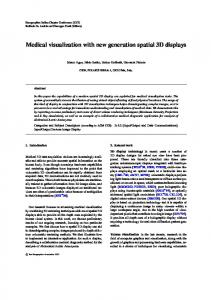
Figure 3.1: Cartographic rendering of roads in Vorarlberg, Austria, and in Munich, Germany.

The efficient and high quality rendering of complex road networks—given as vector data—and high-resolution digital elevation models (DEMs) poses a significant problem in 3D geographic information systems. As in paper maps, a cartographic representation of roads with rounded caps and accentuated clearly distinguishable colors is desirable. On the other hand, advances in the technology of remote sensing have led to an explosion of the size and resolution of DEMs, making the integration of cartographic roads very challenging. In this work we investigate techniques for integrating such roads into a terrain renderer capable of handling high-resolution datasets. We evaluate the suitability of existing methods for draping vector data onto DEMs, and we adapt two methods for the rendering of cartographic roads by adding analytically computed rounded caps at the ends of road segments. We compare both approaches with respect to performance and quality, and we outline application areas in which either approach is preferable. 27

28

3.1

CHAPTER 3. CARTOGRAPHIC ROADS ON DEMS

Introduction

Figure 3.2: Cartographic rendering of road maps using vivid colors and dark edges to achieve a high visual contrast to the underlying terrain.

Geographic Information Systems (GIS) store, analyze and visualize geo-referenced data (see Section 2.1). Road networks, land usage regions and selected points of interest are usually stored as vector data (see Section 2.1.2). In urban planning, cartography, and for navigation purposes, the visualization of roads on digital terrain models plays an important role [Döl05]. GIS engines should be able to handle and display such vector data efficiently and at high quality. A bare and uncluttered visualization as in paper maps is desirable. This cartographic representation of roads requires vivid colors, dark edges, rounded caps and runtime scaling of road width [Kra00; RMMKG95]. Dynamic scaling allows the perception of roads at every distance. In a cartographic rendering, roads are tinted using vivid colors to distinguish them from the underlying terrain. Associating different colors to each type of road induces an automatic cognitive grouping of similar roads [Kra00]. In addition, dark edges around roads add visual contrast [RMMKG95]. Examples of such cartographic representations are shown in Fig. 3.2(a) and 3.2(b). An additional aspect of a cartographic representation are rounded caps at each road segment. This avoids the appearance of cracks between segments and makes the visualization more appealing by introducing smooth endings and avoiding undesirable angular corners. Another important information layer in GIS is the digital elevation model (DEM). It is usually given as raster data defining a 2.5D height map (see Section 2.1.2). Since the resolution and size of these DEMs are increasing rapidly, rendering approaches must be capable of dealing with TBs of data and gigantic sets of primitives that have to be displayed at high frame rates. To cope with these requirements, visualization techniques employ adaptive Level-of-Detail (LOD) surface triangulations [LKRHF+96] and data compression, combined with sophisticated streaming and pre-fetching strate-

3.2. RELATED WORK

29

gies [DSW09]. In such scenarios, the combined visualization of roads and a highresolution DEM in a single visualization engine becomes a challenging task. The main contribution is a method for rendering cartographic roads with rounded caps on high-resolution DEMs. We extend existing vector draping methods by introducing the possibility to compute caps analytically, thus avoiding an explicit triangulation. In this way we achieve a high-quality appearance without increasing the number of geometric primitives to be rendered. Furthermore, we introduce screen-space road outlines, runtime width scaling, and correct treatment of road intersections. We have integrated our method into a tile-based terrain rendering engine. During preprocessing, this engine builds an multiresolution pyramid for both the DEM and the orthoimage. It then partitions each level into square tiles, creating a quad tree. Each tile stores a Triangulated Irregular Network (TIN) representation of the DEM along with the orthoimage During runtime, tiles are chosen based on a maximum allowed screenspace error. In combination, this enables interactive 3D browsing of high-resolution terrain data with superimposed cartographic roads.

3.2

Related Work

Terrain Rendering. Terrain rendering approaches using rasterization have been studied extensively over the last years. They employ the GPU to render large sets of polygonal primitives, and they differ mainly in the hierarchical height field representation used. There is a vast body of literature related to this field and a comprehensive review is beyond the scope of this thesis. However, Pajarola and Gobbetti [PG07] discuss the basic principles underlying such techniques and provide many useful algorithmic and implementation-specific details. A thorough discussion of terrain rendering issues that are specifically related to high resolution fields is given in [DSW09]. Vector Data. The mapping of vector data on DEMs is an active research subject. The existing methods can be broadly classified into geometry-based, texture-based and shadow volume-based approaches. Geometry-based. These methods generate and render separate primitives for the vector data. As the sampling frequency of the vector data generally does not match the triangulation of the underlying terrain, an adaption to the terrain triangulation and its LOD scheme is necessary. Because of this pre-process, geometry-based algorithms

30


are strongly tied to the terrain rendering system and usually only allow static vector data [ARJ06; SGK05; WKWRF03]. Texture-based Approaches. Texturing techniques map the vector data onto a DEM in two steps: first, the data is rendered into offscreen textures either at runtime or in a pre-process. Afterwards, these textures are overlaid onto the terrain using texture mapping [DBH00]. This approach does not produce any aliasing artifacts thanks to hardware-supported texture filtering. Additionally, these methods are independent of the underlying terrain triangulation algorithms. Static texturing methods provide high performance, but do not allow runtime changes of rendering parameters. Further problems occur at large zoom factors, as only limited resolution textures can be pre-computed—there is an inherent tradeoff between the memory requirements and the obtainable quality [DBH00]. Therefore, Kersting and Döllner [KD02] combine this approach with on-demand texture pyramids: associating each quadtree region with an equally sized texture allows on-the-fly generation of appropriate textures. Dynamic vector data can be visualized if these textures are created in each frame. However, this severely impacts performance, as many render target switches are needed. To overcome this, Schneider et al. [SGK05] introduce an approach using a single reparameterized texture for the vector data, analogously to perspective shadow mapping (PSM) [SD02]. As in PSM, some aliasing artifacts occur. Bruneton and Neyret [BN08] present an approach that adapts the terrain heightfield to constraints imposed by the vector data (e.g., to enforce locally planar roads). Their method works only on regular meshes and would be difficult to generalize to our TINbased terrain system. It is also not feasible for high-resolution terrain data. Additionally, an adaption of the heightfield is only necessary if the terrain resolution is insufficient to resolve such constraints, or if real-time editing is desired. Shadow volume-based Approach. This approach, recently introduced by Schneider and Klein [SK07], uses the stencil shadow volume algorithm to create pixel-exact draping of vector data onto terrain models. A stencil mask is created by extruding polygons along the nadir and computing the screen-space intersection between the created polyhedra and the terrain geometry. Using this mask, a single colored fullscreen quad is drawn. For each color, a separate stencil mask has to be generated. However, as the number of different vector data colors is typically small, this is not a major problem. The approach does not require any pre-computations and is thus completely independent of the terrain rendering algorithm. A similar approach was introduces by Ohlarik and Cozzi [OC11]. Instead of creating volumes, they create triangle walls by extruding

3.3. CARTOGRAPHIC ROADS

31

the polyline. In the fragment shader, they use the depth and silhouette of the DEM to generate one pixel-width lines projected onto the terrain. Parametrized surfaces. Large numbers of similar primitives can be rendered efficiently using analytic methods. The main goal is to reduce bandwidth requirements when displaying a large amount of similar elements. Splatting objects to quadrangular approximations and solving their raycasting equation enables GPU-accelerated visualization of glyphs. By using parametrized surfaces, implicit surfaces are generated. For instance, tensor fields can be visualized by ellipsoids [Gum03], solving intersection and shading equations on the GPU. Finally, an implicit generation of hyperstreamlines is done by using a GPU-based sphere tracing with oriented ellipsoids [RBEHE06]. Our goal is to render cartographic roads on a high-resolution DEM. Continuous road scaling is a prerequisite, which makes texture-based approaches unsuitable. Likewise, a runtime triangulation of roads to match the DEM is not feasible, so most existing geometry-based approaches are not usable in our case. We chose to use the shadow volume approach, as it does not require a pre-process and thus allows for runtime scaling of roads. It also provides pixel-exact projections. As a simpler and faster alternative, we also investigate a geometry-based approach where we adapt only the road centerlines to the DEM, so road scaling remains possible.

3.3

Cartographic Roads

In GIS, roads are usually stored as vector data, i.e., as a collection of 2D polylines. One possibility to visualize such data is to convert the vector data into geometric primitives that are rendered on top of the terrain. However, a naive extrusion of each line segment to a quad results in the appearance of cracks between segments. The higher the curvature of a polyline, the more these cracks become visible. Two pragmatic solutions exist: filling the holes with additional triangles (Fig. 3.3(a)) or connecting the corners of adjacent quads (Fig. 3.3(b)). Both solutions are only possible if adjacency information is available. In real datasets, however, this information is commonly incomplete. Fig. 3.4 shows an example from a real dataset where one continuous road is represented by several individual polylines, resulting in cracks between adjacent road segments where the polylines meet. We therefore choose a robust and elegant solution, which draws caps to avoid the appearance of cracks (Fig. 3.3(c)) and does not require adjacency information.

32


(a) Extra triangle

(b) Moving corners

(c) Rounded caps

Figure 3.3: Methods for removing cracks between quads.

(a) Cracks

(b) Fixed with caps

Figure 3.4: Cracks occur because of missing adjacency information.

In addition to filling cracks, this approach generates visually pleasant smooth road endings (Fig. 3.5, top). It also naturally handles sharp turns in a road (Fig. 3.5, bottom). Many major navigation systems visualize roads using rounded caps, for example in Nokia Maps, Apple Maps, Google Maps, Navigon and TomTom. It has become a defacto standard technique when rendering cartographic roads [Nds]. A naive method for

(a) No rounded caps

(b) With rounded caps

Figure 3.5: Quality improvement with rounded caps.

rendering caps is the triangulation of a half-circle, leading to a large number of additional triangles per segment. Furthermore, the discrete triangulation becomes visible at large zoom factors. In the following sections, we present two methods that allow using perfectly round caps while avoiding an increase of the triangle count.

3.4. GEOMETRIC APPROACH

3.4

33

Geometric Approach

Our first method renders cartographic roads using a geometry-based approach. From the initial polyline representation of a road, we individually process each line segment defined by successive vertices. In a pre-process, these lines are clipped against the terrain mesh in 2D, inserting additional vertices at each intersection (Fig. 3.6). For more details on this pre-process, see Section 3.6.1.

(a) Incorrect mapping of a road (gray vertices); problematic areas are marked by spirals

(b) Correct mapping of the road using additional vertices (red)

(c) Top-down view with additional vertices

Figure 3.6: Geometry-based mapping of roads onto a terrain mesh.

To render rounded caps, we do not explicitly triangulate half-circles at the beginning and the end of each road segment. Instead, we render a single quad encompassing an entire road segment and evaluate the caps analytically in a shader program [Gum03] (Fig. 3.7).

(a) Line segment i

(b) Generated quad

(c) Analytical caps

Figure 3.7: Analytical evaluation of rounded caps on a base quadrilateral.

We use the endpoints Pi and Pi+1 of each line segment and the tangent ~ti to generate a quad encompassing both capped ends (Fig. 3.7(a) and (b)). From the tangent vector~ti = (ti,x , ti,y ) we obtain the normal ~n as ~n = (−ti,y , ti,x ).

34


With ~ti , ~n, and the road width w, we compute the two displacement vectors ~t 0 = 0.5 · w ·~ti ,

~n 0 = 0.5 · w ·~n.

With these, we finally compute the four corners Qi0 = Pi +~n 0 −~t 0 ,

Qi1 = Pi −~n 0 −~t 0 ,

Qi2 = Pi+1 +~n 0 +~t 0 ,

Qi3 = Pi+1 −~n 0 +~t 0 .

The caps are cut out of the generated quad in a pixel shader. We create a normalized local coordinate system inside both caps [RBEHE06], which allows determining those fragments of a quad that are outside the cap and have to be discarded (Fig. 3.7(c)). Given points P0 , P1 , the ratio h between their distance d = P0 P1 and the cap radius w2 is given by w w h= . w = (d + 2 · 2 ) d + w Equipped with h, we generate the local coordinates inside the caps with xcap =

|x| − 1 +1 , h

ycap = |y|.

2 + If xcap > 0, the fragment lies inside the cap area (the red area in Fig. 3.7(c)). If xcap y2cap > 1.0, it is outside of the half circle that builds the cap, and is discarded.

3.5

Shadow Volume Approach

Our second algorithm is an extension of the shadow volume-based approach introduced by Schneider and Klein [SK07]. We extrude the road geometry along the nadir and apply a stencil shadow volume algorithm [Cro77; Hei91]. Thus, we compute the intersections between the extruded roads with the terrain geometry, resulting in per-pixel accurate projections onto the terrain. Similar to the approach described in Section 3.4, we extend this algorithm by adding analytic rounded caps. We enlarge the geometry of each line segment to encompass the caps, and construct a local coordinate system that allows us to determine the fragments lying inside or outside the cap area. In the inside area, we analytically evaluate the caps via an intersection test between a ray and a cylinder and compute the depth value of the intersection point to be used during the depth test.

3.5. SHADOW VOLUME APPROACH

3.5.1

35

Intersection

From the camera position O, the fragment position F, and the view direction ~v = (F − O)/ |F − O| we construct the view ray R = O + t~v. Given such a ray, the intersection of the ray with the cylinder spanned by the cap can be computed. Because the cylinder is always aligned with the z axis (the nadir), we can replace the 3D ray-cylinder test by a 2D ray-circle test in the xy plane (Fig. 3.8). A circle with center C and radius r is defined by the equation (X −C)2 = r2 . Inserting the ray R into this equation with ~c := O −C yields ((O + t~v) −C)2 = (~c + t~v)2 = r2 . Expanding this results in the quadratic equation (~v ·~v) t 2 + 2 (~v ·~c) t + (~c ·~c − r2 ) = 0. Solving for t gives the discriminant d = 4 (~v ·~c)2 − 4 (~v ·~v) (~c ·~c − r2 ). If d ≤ 0, there is none or only a single solution to the quadratic equation. This means that the ray does not hit the cap at all, or just grazes it. In this case, we discard the fragment. Otherwise, we get √ −2 (~v ·~c) ± d t1/2 = . 2 (~v ·~v) For front faces, min(t1 ,t2 ) is the correct solution, for back faces it is max(t1 ,t2 ). So far, we have assumed that the road geometry is extruded toward infinity to generate the shadow volumes. Since this is wasteful in terms of rasterization fill rate, we consider the height field for limiting the extent of the shadow volumes. Assuming the terrain being partitioned into tiles, it is sufficient to extrude each line segment only within the extent of the bounding box of the tile it belongs to. Therefore, the intersection algorithm has to be extended to handle the top and bottom sides of the extruded polyhedron: If the 2D distance between F and C is smaller than the cap radius (which can only happen for fragments belonging to the top or bottom side), F already gives the final intersection.

36

3.5.2


Numerical Precision

The algorithm as presented so far suffers from problems caused by limited numerical precision. One such problematic situation is depicted in Fig. 3.8: The intersection between each ray and the cylinder is computed twice, once for the front face of the bounding box (corresponding to F0 in the figure) and once for the back face (corresponding to F1 ). The ray direction is computed as F0 − O and F1 − O, respectively. Because of small perturbations in F0 and F1 , which are caused by the limited precision of the interpolation hardware, one of the intersection tests may report an intersection while the other one does not. This results in inconsistent output causing visible artifacts.

Figure 3.8: Numerically problematic ray-circle intersection.

In order to achieve consistent results, we compute both intersections in the same shader invocation: We render the geometry with front face culling enabled, and analytically compute the entry point into the bounding box of the extruded road. We then compute both intersections between the ray and the road as described above. This results in two depth values z0 , z1 that need to be compared to the terrain depth zt . We therefore replace the regular depth test with a custom two-sided test: zt is read from a texture created as a secondary render target during the terrain rendering pass. If z0 < zt < z1 , then the road volume intersects the terrain geometry; otherwise, we discard the fragment. Two beneficial side effects of this approach are that only half the amount of geometry needs to be rasterized compared to the naive approach, and that in contrast to the original shadow volume algorithm it does not require the rendering of full-screen quads to color the intersections.

3.6. IMPLEMENTATION DETAILS

3.6

37

Implementation Details

In our proposed GIS engine, we visualize vector data from the OpenStreetMap project [Ope] (Chapter 2.1.3). Road networks are stored as a collection of polylines. Each polyline has a functional road class (FRC) [Tal96], defining a distinct width and color. For efficient data management at runtime, we partition the vector data into quadtree tiles, similar to the terrain data. Inside each tile, roads are stored sorted by their FRC. 3.6.1

Geometry Clipping

To avoid an incorrect mapping of roads onto the DEM in the geometric approach as in Fig. 3.6(a), we apply a pre-process where the centerline of each road segment is clipped against the terrain mesh in 2D. Additional vertices are inserted at each intersection (Fig. 3.6(c)). However, finding the exit point of a line in a triangle by line-line intersection tests with the triangle edges provides poor numerical stability. We therefore perform these calculations in barycentric coordinates as illustrated in Fig. 3.9.

Figure 3.9: Computing line – triangle edge intersections.

We trace a line from point P along the normalized vector~v in the triangle defined by the vertices T0 , T1 and T2 . The change in the barycentric coordinate λ2 of P with respect to T2 is given by the signed distance moved along a~0 divided by the distance d0 of T2 from e~0 , where a~0 is a normalized vector perpendicular to e~0 and pointing inside the triangle. When moving along ~v, this becomes (~ a0 ·~v)/d0 . If this value is larger than zero, ~v is pointing away from e~0 and we skip this edge. Otherwise, the maximum distance x0 we can move along ~v before we hit e~0 is given by x0 =

λ2 d0 . a~0 ·~v

This can be done analogously for the other edges to compute x1 and x2 ; the smallest of these provides the actual exit point where an additional vertex is inserted.

38


3.6.2

Geometry Z-Offset

Even after adapting the roads to the terrain, z-fighting artifacts occur when using the geometric rendering approach (Fig. 3.10). Most of these artifacts can be resolved by an additional scaling of the vertices Pi in view space. The vertex transformation thus becomes proj(Pi ) = Pi · W · V · (1 − α) · P, where W, V and P are the world, view, and projection matrices, respectively, and α is a small value > 0 (we used 0.02). In contrast to an offset in world space, this approach does not cause roads to hover when viewed from up close.

(a) Artifacts where roads intersect with triangulated terrain

(b) Resolving artifacts by z-offset

Figure 3.10: Z-fighting between roads and the terrain geometry.

3.6.3

Cartographic Rendering

Scaling. In cartographic rendering, roads should be visible at all zoom levels. Therefore, while zooming out our system scales the roads’ widths continuously. The scaling factor is determined by the distance to the viewer. To avoid that roads close to the viewer become too wide, we only scale roads that are further away from the user than a given distance threshold (Fig. 3.11). Intersections. At crossroads or junctions, multiple roads of potentially different FRCs overlap, resulting in visible artifacts caused by additive blending. To resolve this problem, we draw roads into an offscreen render target without blending, in increasing order of importance. The same approach allows for an easy integration of multi-colored roads by drawing a road multiple times with different widths and colors. This increases the geometry count

3.6. IMPLEMENTATION DETAILS

(a) No scaling

39

(b) Constant scaling

(c) Distance-based scaling

Figure 3.11: Scaling of road width. Without scaling, distant roads become too narrow (left). A constant scale makes close roads too wide (middle). Distance-based width scaling gives satisfactory results (right).

proportionally to the number of colors, but since typically only a few important roads use multiple colors, this is acceptable. Fig. 3.12 demonstrates the correct handling of intersections of roads with different FRCs, including a two-color motorway.

Figure 3.12: Correct handling of road intersections.

Outlines. To distinguish cartographic roads from the underlying terrain, we add dark edges around roads to increase contrast [RMMKG95]. To detect edges in screen space, we use a 3 × 3 or 5 × 5 kernel to find the local maximum road intensity αmax around each fragment. The road intensity is the road opacity for pixels which are covered by a road, and 0 otherwise. The difference αmax − αcurrent defines the resulting edge intensity. Fig. 3.13 demonstrates the increase in visibility achieved by using outlines around roads.

40


(a) Without outlines

(b) With outlines

Figure 3.13: Improving visibility by using dark outlines.

3.7

Results

We have tested the proposed algorithms using three high-resolution datasets: • A DEM of the US State of Utah, covering an area of about 276, 000 km2 at a geometric resolution of 5 m. The road dataset contains about 6, 839, 000 vertices (216 MB). • A DEM of Bavaria in Germany, covering an area of about 70, 500 km2 at a geometric resolution of up to 80 cm. The road dataset contains about 5, 697, 000 vertices (151 MB). • A DEM of the Vorarlberg region in Austria, covering an area of about 4, 760 km2 at a geometric resolution of 1 m. The road dataset contains about 213, 000 vertices (7 MB). The size of the terrain data including orthoimages is around 1 TB per dataset. We therefore use an out-of-core visualization system capable of handling arbitrarily large datasets. The pre-processing step for the geometric approach (see Section 3.6.1) increased the size of the road data by about a factor of ten in all tested cases. Note that for the shadow volume approach, this step is not required. Performance. All performance measurements were taken at a display resolution of 1600 × 1200 on a PC with Windows Vista, a 2.66 GHz Intel Core 2 Quad CPU, 8 GB of RAM and an ATI Radeon HD 5870 GPU (driver version 10.6). The results can be seen in the following Fig. 3.14. The graph in Fig. 3.14(a) shows the frame rate during a recorded flight over the mediumresolution DEM of Utah at an average speed of about 1750 m/s. When rendering geometric roads (GEO), the maximum (average) performance drop is about 30% (26%)

3.7. RESULTS

FPS

No roads

400

41

GEO, no caps GEO, caps

SV, no caps SV, caps

FPS

GEO, no caps GEO, caps

No roads

300

SV, no caps SV, caps

250

300

200

200

150 100

100

50

0

0 0

100

200

300 Time (s)

(a) Performance - Utah.

400

500

0

50

100

150 200 Time (s)

250

300

(b) Performance - Bavaria.

Figure 3.14: Benchmark of GEO and SV in the medium-resolution DEM of Utah and the high-resolution dataset of Bavaria.

compared to rendering the terrain without roads. The highest performance impact occurs over Salt Lake City (far right in the graph). This area contains a dense road network and only a small amount of terrain geometry, as buildings are not included in the height field. The additional rendering of rounded caps does not significantly influence the performance. For shadow volume-based roads (SV), the maximum (average) performance drop is around 40% (35%) without and 55% (42%) with rounded caps. Breaking the numbers down to the sole rendering of roads, SV with caps is about 1.4 times as expensive as without caps. The visual quality produced by both techniques is identical at most locations in Utah. Therefore, GEO is preferable because of its higher performance. Fig. 3.14(b) shows the frame rates during a flight over the high-resolution dataset of Bavaria at an average speed of about 950 m/s. In this scenario, the performance of all approaches is very close; the average cost is between 33% and 43%. Even though GEO often requires many more triangles (up to about 3 million) than SV (≤ 1M) because of the adaption to the terrain mesh (which itself uses up to about 35M triangles), GEO is still slightly faster. Thus, the GPU is more limited by shading computations than by the geometry throughput. However, GEO can often not provide an adequate mapping on such high-resolution terrain data (Fig. 3.15). Therefore, SV is preferable for such fine-grained DEMs. The Vorarlberg dataset has a similar geometric resolution as the Bavaria dataset, but the road network is much more sparse. Regardless of which algorithm is chosen for rendering roads, the highest performance impact amounts to only 15%. However, as in Bavaria, GEO cannot provide adequate quality.

42


(a) Geometric

(b) Shadow volume

(c) wireframe

Figure 3.15: Comparison of our draping algorithms on high-resolution terrain.

Matching. We should note that in many situations the vector dataset did not exactly match the terrain data, i.e., there was a certain offset between the vector data roads and roads in the orthoimages. These problems frequently occur in cities or forests, where even a slight offset causes a road to be projected onto a building or a tree. GEO fails to produce any reasonable results in this case (Fig. 3.16(a)); SV produces a technically correct but not very useful projection (Fig. 3.16(b)). This is a problem of the data rather than the draping algorithm. An additional pre-processing step could match the vector data to the terrain and its orthoimages.

(a) Geometric

(b) Shadow volume

Figure 3.16: Artifacts caused by a mismatch between terrain and vector data.

Comparison. Our method presents a marked improvement over several commercial GIS systems. For example, Google Earth 6.2 uses a simple geometric approach without adaption to the terrain and therefore does not achieve a correct projection of roads onto the DEM. It also does not provide correct road intersections and does not support multicolor roads or outlines. ArcGIS 10.0 rasterizes vector data into textures which are overlaid onto the terrain, similar to the orthoimages. This results in a correct projection and correct behavior at road intersections. However, a dynamic scaling of road widths is not possible, and multi-color roads or outlines are not supported.

3.8. CONCLUSIONS

3.8

43

Conclusions

We have proposed and evaluated two approaches for rendering high-quality cartographic roads with rounded caps on high-resolution 3D terrain models. Both can be used on hardware platforms supporting Direct3D 10 or OpenGL 3.2. We have shown that a geometry-based approach provides high performance and good quality for lowto medium-resolution terrain datasets. However, it requires a moderately complex preprocessing step, and it cannot provide an adequate visual quality with high-resolution terrain data. It is therefore a reasonable choice for low-end hardware, e.g., on mobile devices, where rendering of high-resolution terrain data is not feasible. The shadow volume algorithm enables pixel-exact rendering of cartographic roads on 3D terrain. It is more expensive at runtime than the geometry-based approach; however, the rendering of high-resolution terrain remains the larger part. In low-resolution terrain datasets, on the other hand, its relative performance impact is large. The algorithm is easy to integrate into existing terrain rendering engines, as no adaption of roads to the terrain is required. It also extends naturally to polygonal vector data. In further research, we plan to evaluate the use of tessellation shaders for the creation of geometric caps on Direct3D 11 or OpenGL 4.0 capable hardware.

44


Chapter 4

Temporally Coherent Real-Time Labeling of Dynamic Scenes

(a) Annotation of a large graph network.

(b) Labeling a GIS in Geneva, Switzerland.

Figure 4.1: Real-time labeling of 2D (left), 3D (right) scenes using our force-based approach.

The augmentation of objects by textual annotations provides a powerful means for visual data exploration. Especially in interactive scenarios, where the view on the objects and, thus, the preferred placement of annotations changes continually, efficient labeling procedures are required. As identified by a preliminary study, these procedures have to consider a number of requirements for achieving an optimal readability, e.g., cartographic principles, visual association and temporal coherence. We present a forcebased labeling algorithm for 2D and 3D scenes, which can compute the placements of annotations at very high speed and fulfills the identified requirements. The efficient labeling of several hundred annotations is achieved by computing their layout in parallel on the GPU. This allows for a real-time and collision-free arrangement of both dynamically changing and static information. We demonstrate that our method supports a large variety of applications, e.g., geographical information systems, automotive navigation systems, and scientific or information visualization systems. We conclude this chapter, with an expert study which confirms the enhancements brought by our algorithm with respect to visual association and readability. 45

46

4.1

CHAPTER 4. TEMPORALLY COHERENT LABELING

Introduction

Information can be represented by images and textual annotations. Images give a quick overview and portray data intuitively. In contrast, textual annotations have to be actively read. However, they can precisely describe objects with selected information. Combining both types creates a very powerful tool for data exploration. These principles are used in the fields of information visualization and visual analytics. Therein, abstract data is often described by textual annotations. For instance, graphs with up to several hundred nodes have to be labeled (see Figs. 4.1(a) and 4.9). Another area of research focuses on geographic information systems (GIS) (see Section 2.1). These systems visualize geospatial data such as road networks, demographic data, and their annotations (see Figs. 4.1(b) and 4.6(b)). An example is our proposed map viewer framework introduced in Chapter 3 which renders cartographic roads on high-resolution DEM. Such systems, especially when used on large-scale display systems, must be able to provide interactive visual exploration of geospatial data with a very high number of annotations. Since in such 3D (or 2.5D) applications the camera can be moved freely, the use of unconstrained labels and the pre-processing of every possible layout constellation to avoid collisions is impractical [Mot07]. More and more such applications have to cope with dynamic content, requiring placements of labels without prior knowledge, e.g., when loading KML files into Google Earth. Therefore, real-time computation of annotation layouts is becoming an ever important requirement in interactive data exploration. Besides interactivity, additional requirements such as Imhof’s cartographic principles [Imh75] have to be considered to improve the visual analysis process. Adhering to these principles, including readability, visual association, and classification, is extremely challenging and demands for a proper integration of the respective functionality into label placement algorithms, e.g., support for scalable rotated labels with priorities. In addition, only a stable and consistent (similar to [BDY06]), as well as temporally coherent layout, where labels do not jitter, appear suddenly, or move unexpectedly, lets users easily track annotations in a complex scene. Labels should make slow-paced, smooth transitions to minimize distraction. Therefore, on top of the aforementioned requirements, the maintenance of a frame-coherent presentation is another major concern underlying our developments. In many applications the demand for a temporally coherent layout even supersedes the requirement for an optimal position in every frame.

4.2. RELATED WORK

47

Based on our intended application areas and a preliminary study (see Section 4.3), we define the following goals: • Real-time labeling of point, line and area features • Runtime placement of new labels • Scalability to up to several hundreds of labels • Temporal coherence and stability of the labeling layout • Consideration of Imhof’s cartographic rules, e.g., readability, visual association and classification • Support for rotated and scaled labels with priorities Most existing real-time approaches follow the first two rules but do not scale well with the number of labels, have problems maintaining temporal coherence, and do not rigorously adhere to common cartographic rules (see Section 4.2). The major contribution is an efficient algorithm for creating a temporally coherent labeling of 3D or 2.5D objects and scenes. Our algorithm is specifically tailored to the massively parallel multi-threading architecture of graphics processing units (GPUs). Every label collision is detected with the separating axis theorem computed in parallel on the GPU. Collisions between labels are resolved with a force-based approach thus creating smooth changing label positions. In this way we can create layouts for several hundred annotations in real-time. Furthermore, our method supports scaled and rotated annotations.

4.2

Related Work

Cartographic principles. Imhof [Imh75] names legibility and the graphical association of a label with its feature as characteristics of good lettering. Furthermore, he emphasizes the importance of minimal map disturbance, good label distribution, as well as fonts which indicate the spatial properties of features and their classification. He divides the labeling problem into three categories: labeling point features, line features and area features. For each category certain cartographic principles apply. Yoeli’s four-position model [Yoe72] depicted in Fig. 4.3(a) ranks each possible position of a label around a point feature according to its degree of intuitive association. He already mentions the semi-automatic labeling of point features. Its computational complexity is

48


NP-complete [MS91]. Christensen et al. [CMS95] introduce the point-feature-labelingproblem (PFLP) and prove that it is NP-hard. Thus, heuristics are needed to label maps with a huge number of features. A broad range of strategies has been developed, for instance exhaustive rule-based, genetic, force-based or greedy approaches. A collection of related papers can be found in the bibliography by Wolff and Strijk [WS12]. Force-based. A force-based approach was first presented by Hirsch [Hir82]. He uses a gradient-driven heuristic to label point features. Labels are placed on a circle around their corresponding features. To resolve conflicts, vectors between overlapping labels are computed based on the intersection area. As a single label can collide with multiple other annotations, the sum of all its vectors guides its movement, thus improving the global labeling layout. Feigenbaum [Fei94] describes a similar method to automatically annotate point features. He resolves collisions and places labels close to their anchor by a force-based approach. Attractive forces pull labels to their point feature, while repelling forces push labels away from other features. Thus, step by step, the map layout converges towards a final labeling state through a gradient descent method. Ebner et al. [EKW03; EKW05] enhance this approach by simulated annealing. Consequently, local minima which usually prevail in greedy force-based methods can be avoided. Similar to the approaches of Hirsch and Feigenbaum, this technique approximates the intricate form of a label’s lettering by an axis-aligned rectangle. A hybrid approach is presented by Stadler et al. [SSB06]. They obtain an initial placement with the help of image processing. Then, iterative forces improve the chosen labeling positions. They note that force-based approaches achieve a clear label distribution and thus an aesthetic layout. However, this method does not allow for real-time placement of labels. 2D Real-time. Full interaction with 2D GIS environments, which includes panning and zooming, requires dynamic map labeling. In the last decade, several real-time algorithms for 2D maps have appeared. They divide the labeling problem into a pre-processing and an interactive real-time phase [BDY06; Mot07; PGP03; YCL05]. In the former, a conflict graph is generated which stores every possible conflict between labels at every possible scale. At runtime, relevant labeling positions are chosen based on the pre-computed graph. Unfortunately, all these approaches only work for a topdown view and require uniformly sized, axis-aligned labels. Recently, real-time labeling of 2D maps without pre-processing has been achieved by Luboschick et al. [LSC08; CLS09]. They divide the available screen space into a uniform grid wherein “conflict particles” indicate if a region (cell) is occupied. Choosing a labeling position then becomes a search for free cells. This approach uses existing position-models [Yoe72]

4.2. RELATED WORK

49

sequentially to determine the first valid position. By using particles, this method can freely define obstacles and is not restricted to axis-aligned annotations. The layout is computed from scratch every frame. Temporal coherence is achieved by interpolating the resulting positions. However, during animation, occlusion of labels can occur. In this approach, most of Imhof’s cartographic principles [Imh75] are not addressed, even though positioning models are used. 3D Real-time. Bell et al. present a real-time approach for labeling a 3D virtual world [BFH01]. They introduce the notion of temporal continuity in a lettering. This avoids popping of annotations while panning or zooming the map. Labels are projected from 3D world space into 2D screen space. Placement is done by iterating through a set of rectangles describing unoccupied screen space. Thus, the performance of this method does not scale well and labels can only be approximated by axis-aligned rectangles. A simpler approach from Maass and Döllner [MD06b] splits the screen space into disjoint vertical slots. Therein, labels are stacked sorted by their distance to the viewer. A line connects a feature and its label visually. A bold font with a halo makes textual annotations easily readable. However, this approach creates dense clusters of labels and long connecting lines. Thus, visual association becomes impossible. Several approaches deal with the labeling of single 3D objects for illustration purposes [AHS05]. Göetzelmann et al. [GHS06] describe an algorithm which uses distance fields to compute ideal labeling positions and employ agents to preserve temporal coherency. Unfortunately, during camera movements labels are hidden and jittering occurs. Stein and Décoret [SD08] present a GPU-based real-time approach for labeling a 3D scenery. To compensate the drawbacks of their greedy approach, an Appolonius diagram defines the label placement order. Similar to Stadler et al. [SSB06], they use image processing to determine the initial positions. Unfortunately, only up to 20 labels can be placed at interactive frame rates. Furthermore, during navigation, jittering and harsh changes in labeling positions occur. Finally, a real-time approach for annotation of virtual reality environments is described by Pick et al. [PHWTPK10]. They choose the initial position of a label by voxelizing the corresponding object, extracting a medial line and choosing the closest point on this line to the object’s center of gravity. Unfortunately, this can lead to collisions at placement and thus unstable layouts. To resolve conflicts at runtime, they first compute a visibility volume from an object’s axis-aligned bounding box. The intersection between these volumes on directed 2D planes creates a force vector which depends on the penetration depth. This force is applied at runtime on the involved labels. However, real-time labeling can only be achieved for 20-40 annotations.

50


Summary. None of the presented approaches satisfy all the requirements stated in Section 4.1. Several real-time algorithms suffer from visual frame-to-frame discontinuities and create too much movement in the labeling layout [MD06b; SD08]. Others only follow a minor set of Imhof’s cartographic principles [CLS09; LSC08; MD06b] or exhibit an unstructured layout [CLS09; MD06b; PHWTPK10]. The performance of some approaches does not scale well [BFH01; SD08; PHWTPK10]. Finally, some algorithms only allow axis-aligned annotations [BFH01; Mot07; MD06b; PGP03; SD08; PHWTPK10].

4.3

Preliminary Study

A good readability is one of the most important goal of our approach. In order to define design principles, we conducted a preliminary expert study at our research facility. As a representative application, we chose the labeling of a GIS with 3D-terrain overlaid by orthoimages and a road network. We interviewed one psychologist, who has been working as a researcher in the human-machine interaction (HMI) design field for over two decades, four engineers, three of which work as project leaders for navigation components, the fourth is developing HMI concepts, and a sixth expert who has worked for over a decade as a visual designer. 4.3.1

Study Design

In an interview of approximately one hour we presented different labeling concepts (Fig. 4.2), all adhering to Imhof’s cartographic principles [Imh75], and we provided the following questionnaire to the experts. First, we asked whether the size of a label should change with respect to its depth position in a 3D landscape. Second, we surveyed how to annotate point features (e.g., cities): using the four-position model, centered above their anchor, or circling around its feature. Finally, we questioned the best strategy to label line features (e.g., streets): horizontally (Fig. 4.2(a)), as rotated straight labels (Fig. 4.2(b)), or by following the line features (Fig. 4.2(c)). 4.3.2

Results

Depth Scaling. This concept categorizes the subjects into two groups. The first group (with 4 of 6 candidates) stated that depth scaling helped spatial perception in the 3D landscape. The second group (2 of 6) stated it is acceptable if textual annotations remain readable.

4.3. PRELIMINARY STUDY

(a) Horizontal annotations.

51

(b) Straight, screen space rotated an- (c) Annotations following the roads notations. curvature.

Figure 4.2: Static images for the conducted expert study: each concept shows a different annotation style.

Annotation of Point Features. First, we asked which point labeling concept is appropriate. The majority (4 of 6) stated that a consistent approach was the most important property. Three of the candidates suggested that the labeling concept should create a clear layout and give a good overview of the situation. Finally, one of them chose the 4-position model as the best concept because it incorporated all these stated requirements. Annotation of Line Features. The concept of horizontally placed labels again splits the candidates into two groups. The first group (4 of 6) qualified it as very readable but with a higher search and visual association time. The second group (2 of 6) did not like this kind of placement. One stated reason was that a horizontal label could occlude neighboring features. The concept of straight, rotated annotations was selected as the best alternative by almost every subject (5 of 6) as it provides a good compromise between readability and visual association to the line feature. In the last concept, annotations follow the curvature of the corresponding line. The majority (5 of 6) liked the appearance, but questioned if it would remain readable under special circumstances, e.g., roads with tight turns. Furthermore, this group stated that this concept helps understanding the layout of a road. Some of them (3 of 6) indicated the good visual association. Finally, some (2 of 6) said that they did not see much difference compared to straight annotations. 4.3.3

Design Principles

The first conclusion of our study is that scaling annotations by their depth helps spatial perception in a 3D landscape. However, the scale factor should not go below a certain minimum to maintain readable labels. Hence, the first requirement for the layouting algorithm is freely scalable annotations. Second, labeling point features should create a clear layout and give a good overview of the situation. Therefore, we choose the

52


four-position model because of its clear and consistent labeling. The best compromise between readability and visual association in most situations are provided with straight, rotated labels. Only at very steep angles, where the readability would be compromised significantly, we switch to horizontal labels. Thus, we concluded on the support for rotated annotations as our last requirement. s'i

1

1

p'i

p'i

1

p'i

(a) Horizontal point annotations: The four-position model [Yoe72] defines candidate positions ranked by their degree of intuitiveness, e.g., viewers associate most easily a label with its point feature p0i , if it is placed in the top right corner.

(b) Horizontal line annotations: To label line features at their anchor p0i we can choose between one of three candidate positions.

(c) Rotated line annotations: Three candidate positions for labeling line features along the projected segment s0i . The first candidate position is above p0i , the second candidate is on the right side and the third on the left side.

Figure 4.3: Initial placement of annotations.

4.4

Force-Based Labeling

In this section, we introduce our force-based, real-time labeling approach for dynamic scenes. By providing a temporally coherent layout, at the same time considering the additional requirements identified in the expert study, optimal readability of annotations is enforced in an interactive environment. However, achieving this for a huge number of labels is extremely challenging, since at runtime initial label positions have to be computed (see Section 4.4.3), collisions have to be detected (see Section 4.4.4), and these collision have to be resolved in a temporally coherent manner (see Section 4.4.5). 4.4.1

Motivation

According to Chen et al. [CPB04], naive search tasks are completed in less time when labels are displayed in screen space. Hence, to achieve an optimal readability and

4.4. FORCE-BASED LABELING

53

a more efficient visual exploration we handle the entire layouting in screen space. It is worth noting that this strategy also facilitates an efficient computation of conflict situation between different labels [BFH01; LSC08; SD08]. Textual labels and icons are represented by 2D object-oriented bounding boxes (OOBBs) to accelerate the computation of possible collisions via the separating axis theorem [SE02] (see Section 4.4.4). Furthermore, OOBBs enable us to efficiently approximate rotated labels needed for line aligned annotations. For the initial placement of point features, we use the four-position model (see Section 4.4.3). As shown in our preliminary study, and also stated by Yoeli [Yoe72], this model helps creating a visual association between a feature and its annotation. While browsing through annotated datasets, the addition and removal of labels changes the optimal labeling layout, such that in every frame a completely new arrangement might be required to again achieve optimality. These frame-to-frame changes lead to jittering effects and abrupt re-layouting in several existing approaches [LSC08; SD08]. Therefore, we do not create a discrete optimum arrangement in each frame. Instead, the current layout is always based on the labeling result of the previous frame. This is achieved by using a force-based approach which only allows continuous changes to the layout and thus, creates a temporally coherent labeling. Additionally, this results in an appropriate label distribution and avoids clustering [SSB06] (see also Imhof’s cartographic principles [Imh75]).

4.4.2

Features

Following the definition of Imhof [Imh75], 2D/3D scenes contain point features (e.g., graph nodes, Points-of-Interest), line features (e.g., graph edges, streets), and area features (e.g., graph regions, land cover). Point features can be depicted by icons or horizontal labels (Fig. 4.3(a)). Line features can either be labeled horizontally for better readability (Fig. 4.3(b)) or using rotated text following a line segment to create a better visual association (Fig. 4.3(c)). The labels of area features are always drawn horizontally (Fig. 4.3(a)). When loading feature datasets, we first have to compute their labeling positions. Horizontal labels for point features use the feature’s world coordinate p point as the labeling anchor. Line features with horizontal annotations use the polyline’s center pline as the anchor. For a line feature with rotated text, we determine the longest straight segment sline = (pline0 , pline1 ). Finally, for an area feature we compute and store its barycenter parea .

54

4.4.3


Initial Placement

The initial placement of labels consists of choosing a position in screen space when a label first appears. The priorities of labels determine the order of their initial placement. First, we compute the screen space position p0i by projecting the 3D world coordinate pi of a feature’s anchor point. Based on the projected coordinate and the label’s size, we then create an OOBB approximation. As concluded from our expert study in Section 4.3.3, we use the four-position model to label point features. For each of the four candidates k we compute the corresponding OOBB Ck using a screen space offset oi (k) from the projected position p0i (Fig. 4.3(a)). The same is done for area features, using the projected barycenter as the anchor. To consistently place line features, we compute three offset OOBBs Ck from p0i . Depending on the current view angle, the candidate OOBBs are either placed horizontally (Fig. 4.3(b)) or along the projected segment s0i (Fig. 4.3(c)). Each of these candidates (i) k with OOBB Ck of the currently processed label i are tested for collision against the OOBB C( j) of every already placed label j (see Section 4.4.4). If multiple candidate (i) OOBBs Ck are collision free, we choose the position with the best visual association as described by Yoeli [Yoe72]. If there is no free position, we do not add the label i. A timer is started and the initial placement is re-evaluated after the timer expires. To comply with the requirement of a temporal coherent layout from Section 4.1, the new label i is smoothly alpha-blended into the layout. As the placement is ordered by importance, the most relevant annotations are placed in the layout first. Less important labels are filtered out. Enforcing their placement would lead to problems such as collision and clustering. Collision would create rapid movements during conflict resolution, and it would lead to several unreadable labels as stated by Wolff [Wol99; DKSW02, p. 3-4]. Finally, the resulting clusters would make visual association and reading difficult (see Noyes [Noy80] and Imhof [Imh75]). These points would contradict our goal to follow Imhof’s cartographic rules [Imh75]. 4.4.4

Collision

We use a unified approach to layout the labels of all feature categories. Thus, we can involve all feature types to compose the final layout. First, we project all computed positions p point , pline , parea , pline0 and pline1 from 3D world space to 2D screen space, resulting in the projected coordinates p0point , p0line , and p0area , and a projected segment s0line = (p0line0 , p0line1 ) (normalized sˆ0line ). Second, we generate an OOBB encompassing each label. Finally, we compute pair-wise screen space conflicts between all visible


55

oi r

oi

oi ai

p'i

s'i

p'i

(a) Circling annotations: At runtime, a label i with offset oi can circle around its point feature p0i . A spring keeps the label at a distance r from p0i .

(b) Free annotations: At runtime, a label i can freely move away from its optimum position p0i + ai . When no force is acting, the spring repositions the label from p0i + oi to p0i + ai .

d

p'i

(c) Line annotations: At runtime, the label follows the projected screen space segment s0i . A spring positions the label at a distance d from the line s0i .

Figure 4.4: Force-based resolution of collisions.

OOBBs. Implementation details are discussed in Section 4.5. Every OOBB intersection causes the creation of a force vector fcollision which aims to resolve the collision (Fig. 4.5). + f collision

- f collision

Figure 4.5: Collision dependent force vector fcollision .

Collisions between OOBBs are computed using the separating axis theorem [Got00; SE02]. It states that if two boxes do not overlap, there must be an axis which separates their projections. First, we normalize the edge vectors of an OOBB with corners C = {c0 , c1 , c2 , c3 } to unit length and get the set of normalized axes aˆ . Then, we project all its corners C onto every normalized axis. The result is the following interval I: I = [imin , imax ] = [min{â · ci ∈ C}, max{â · ci ∈ C}]

(4.1)

There is no collision between two OOBBs C(n) and C(k) if there exists a normalized axis aˆ in which the respective intervals I (n) and I (k) do not overlap. Thus, there is no

56


(n,k)

collision if for δ0

(n)

(k)

(n,k)

:= imin − imax and δ1

∨

δ0 > 0

(k)

(n)

:= imin − imax : δ1 > 0

(4.2)

To normalize the difference vector δ = (δ0 , δ1 )T to [−1, +1], we calculate the width in relation to the current projection axis as w = −(δ0 + δ1 ) δ g = 2 · ( + 0.5). w

(4.3) (4.4)

Finally, we have to invert the vector to compute the final force with magnitude |f| ∈ [0, 1]. Thus, the magnitude of the resulting force scales with the amount of overlap:  g · ( 1 − 1) if | gy | > 1 gx |gy | (n,k) f = (4.5) g · ( 1 − 1) else |gx |

Analogously to Hirsch [Hir82], we accumulate all collision forces f(i,k) (i 6= k) for every visible label i, resulting in a label’s overall repulsion force (i)

fcollision = ∑ f(i,k)

for i 6= k

(4.6)

k

(a) Annotation layout created by Google Earth: not enough labels are placed, most labels cannot be read properly and camera movement makes labels jitter.

(b) Labeling of a road network in a GIS. In this figure, we define a large buffer zone around the labels to enhance readability and visual association.

Figure 4.6: Comparison of annotation layouts created by Google Earth (left) and using our real-time labeling approach (right). Lettering (color, size, font) and temporal coherence directly impacts the readability and visual association of annotations.


4.4.5

57

Forces and Movement (i)

After calculating the collision forces fcollision for every visible label i, we resolve conflicts using a force-based approach. This enables the flexible definition of each label’s reaction to its surrounding environment. At timestep t every visible label i stores its current screen space offset oi from the projected position p0i , and its velocity vi . First, (i) we compute the total force ftotal acting on the label i. It is composed of several forces, depending on the type of the annotation. In the following, several possible annotation behaviors are introduced: a free annotation, a line annotation and a circle annotation behavior.

Free Annotation. A free label i is positioned by an optional offset ai from its projected anchor p0i (Fig. 4.4(b)). When a collision with force fcollision occurs, it can be repelled in any direction to an offset oi . Its new screen space position becomes p0i +ai +oi , and an attracting force f f eature pulls the label back to its original position p0i + ai . This force f f eature is modeled as a spring with the constant k1 as in Hooke’s law: (i)

f f eature = −k1 · oi

(4.7)

Finally, we introduce a friction force f f riction to stabilize the force-based system. Based on the current velocity vi and a friction coefficient c, we get (i)

f f riction = −c · vi

(4.8)

The total force acting on a free annotation i thus becomes (i)

(i)

(i)

(i)

ftotal = fcollision + f f eature + f f riction

(4.9)

Line Annotation. At runtime, labels for line features can follow a straight segment si in screen space. This is achieved by adding two stiff springs which create the forces fnormal and ftangent . fnormal pushes the label displaced by dreal0 from its optimum distance doptimum along the normal back onto the line. ftangent attracts the label along the line back onto its anchor. Using the projected and normalized line segment sˆ0i , the offset oi and the line equation p = p0i + t sˆ0i , we compute the nearest point pnearest on the line

58


using pnearest0 = p0i + t sˆ0i

oi · sˆ0i |ˆs0i |2 = ||pnearest0 , p0i + oi || t=

with

dreal0

(4.10) (4.11)

Using the normal sˆ0normal = (−sˆ0iy , sˆ0ix )T , the spring constant k2 and the displacement (dreal0 − doptimum ), we compute (i)

fnormal = −k2 · (dreal0 − doptimum0 ) · sˆ0normal

(4.12)

The spring force ftangent with the constant k3 , pulling the label back to its center position, is computed analogously. pnearest1 =

p0line + t sˆ0normal dreal1

oi · sˆ0normal with t = 0 |ˆsnormal |2 = ||pnearest1 , p0i + oi ||

ftangent = −k3 · dreal1 · sˆ0i

(4.13) (4.14) (4.15)

The total force acting on a line annotation i thus becomes (i)

(i)

(i)

(i)

(i)

ftotal = fcollision + fnormal + ftangent + f f riction

(4.16)

Circle Annotation. Similar to Hirsch [Hir82], we introduce an annotation which circles around its anchor. We define a spring with force fcircle keeping the label on a radius r around the projected anchor p0i . Using the distance |oi | between the current position and the anchor, the displacement from the equilibrium is (|oi | − r). The restoring force fcircle with the spring constant k4 and the normalized offset direction oˆ i is (i)

fcircle = −k4 · (|oi | − r) · oˆ i

(4.17)

The total force for a circle annotation thus becomes (i)

(i)

(i)

(i)

ftotal = fcollision + fcircle + f f riction

(4.18)

4.5. IMPLEMENTATION

4.4.6

59

Acceleration

We define a virtual mass mi for each label i. Its value is determined by the label’s importance. The current acceleration ai is computed using Newton’s second law of motion: (i) ai = ftotal /mi (4.19) Each label i has a screen space offset oi at time t. The time difference between consecutive frames is given by ∆t. We obtain the new velocity v0i and the offset o0i at time t + ∆t from Euler’s integration method:

4.5

v0i = vi + ai · ∆t

(4.20)

o0i = oi + v0i · ∆t

(4.21)

Implementation

We integrate this labeling algorithm into our map viewer presented in Chapter 3, which renders cartographic roads and high-resolution DEM. To achieve real-time labeling, we need an efficient computation and resolution of conflicts between labels. We therefore use the GPU for parallel processing of these tasks. Additionally, by using the GPU, we ease the central processing unit (CPU) utilization. As a consequence, the CPU is free to aid in loading, filtering and selection of annotations. The current implementation was done in C/C++, uses OpenGL 3.0 and GLSL. The initial placement of labels is a sequential problem, as we do not want to place multiple labels on the same free spot. To minimize the computational load, this task is split over consecutive frames. In every frame we place a fixed number of annotations. 4.5.1

Parallelization

Every label is an independent entity, similar to a particle. Its properties include the current screen space offset, the velocity, the dimension and the mass. These are stored in a global texture buffer object (TBO). First, we use a GPU kernel to project all anchors of visible labels to screen space. Then, using each label’s current offset oi and its dimensions, we write updated OOBB corners in a TBO. In the second step, a GPU kernel computes the collision between every label pair (n, k) using the separating axis theorem (see Section 4.4.4). This results in a 2D buffer containing force vectors. A (n,k) cell in row n, column k contains the force fcollision created by the collision between the

60


(i)

OOBBs n and k (see Table 4.1). To determine the final force fcollision acting on a single label i, we use a line-wise reduction operation. Label i

(i)

ID 1

ID 2

ID 3

fcollision

ID 1

x

(0.0, 0.0)

(0.5, 0.0)

(0.5, 0.0)

ID 2

(0.0, 0.0)

x

(0.1, 0.3)

(0.1, 0.3)

ID 3

(0.5, 0.0)

(-0.1, -0.3)

x

(0.4, -0.3)

Table 4.1: Pairwise collision creates force (i) fcollision acting on a label i.

(n,k)

fcollision

. Accumulation gives a global collision force

Finally, as described in subsection 4.4.5, we resolve conflicts by applying the force (i) (i) ftotal onto its respective label i. The computation of ftotal and the necessary Euler step for moving the offset oi of a label is done on the GPU. Unfortunately, the precision of Euler’s method is strongly tied to ∆t. Large values lead to an unstable layout. Thus, labels are subject to harsh position changes. Implementing the fourth order RungeKutta method did not lead to significantly better results. In the end, clamping the final acceleration value ai was enough to achieve stability. This leads to continuously moving labels and thus temporal coherent labeling. 4.5.2

Rendering Textual Annotations

After we have determined the current screen position of visible annotations, we render them in a standard way using texture mapped text [Kil97]. However, annotations can surface over complex colored background (Fig. 4.7). Therefore, to achieve a good legibility, we need to carefully choose the font’s appearance. • As stated by Philipps et al. [PNA77], choosing large-sized types helps legibility. Character height can be determined using Smith’s bond rule [Smi79]. • Lower case labels with a large initial capital are more easily found in a map than labels in capital letters only [Phi79]. • As stated by Subbaram [Sub04], a typeface designed for screen display should be selected to improve legibility, e.g., Georgia or Verdana. • A sans-serif typeface is preferred for displaying labels on digital displays [Sub04]. This is not mandatory, as there is still a debate over this matter. • Finally, to save screen space, the chosen typeface should be narrow.

4.5. IMPLEMENTATION

61

To improve readability, we introduce further techniques: We add a dark outline to the font to increase the contrast to the background [RMMKG95] (Fig. 4.7(a)). A halo around the text clears the space around the label and makes it more readable [O’B10] (Fig. 4.7(c)).

(a) Blank.

(b) Dark edge.

(c) Halo.

Figure 4.7: Techniques for increasing the readability of annotations. The best readability is achieved by adding an outline and a halo around the label.

4.5.3

Enhancements

To further stabilize the labeling layout, we implement the following enhancements. Enhanced OOBBs. Changing the view in a scene with a tight labeling layout creates a lot of movement. We remedy this by implementing two improvements: First, we slightly increase the size of the OOBB encompassing each label to create a buffer zone. Second, we define an even larger zone around visible labels where no new annotations can be placed. The latter improvement greatly stabilizes the labeling layout, but has to be used cautiously to avoid filtering out important labels. Speed-based removal. To further stabilize the layout, we remove labels that would otherwise be moving at very high speed. We also remove labels where the different forces acting on them cancel each other out to a large degree, indicating that the label is constricted from multiple sides. The removed labels are inserted again after a given time if there is room for them. These actions help to meet our requirements from Section 4.1, where we stated that labels should make only slow-paced, smooth transitions.

62


Collision

Placement

Other

Total 10

30

8

Miliseconds

Miliseconds

Total 40

20 10 0

Collision

Placement

Other

6 4 2 0

0

500

1000 Number of Labels

1500

2000

(a) Benchmark on low-class hardware: Intel Core 2 Duo 1.6 GHz, 4 GB RAM, Nvidia GeForce 8600M GT (256 MB).

0

500

1000 Number of Labels

1500

2000

(b) Benchmark on lower medium-class hardware: Intel Core 2 Quad 2.66 GHz, 4 GB RAM, Nvidia GeForce 8800GTS (512 MB).

Figure 4.8: Benchmarks of our force-based approach. The plot shows synced timings for the layout computation steps: total labeling time (black), collision computation and resolution (violet), placement of new labels (green) and the overhead generated by other steps (gray). The computation of layouts for several hundred labels remains interactive on every hardware.

4.6

Results

In this section, we analyze our force-based labeling approach with respect to scalability and cartographic principles. 4.6.1

Scalability

We evaluated the performance on two platforms: • low-class hardware: Intel Core 2 Duo 1.6 GHz, 4 GB RAM, Nvidia GeForce 8600M GT (256 MB) • lower medium-class hardware: Intel Core 2 Quad 2.66 GHz, 4 GB RAM, Nvidia GeForce 8800GTS 512 (512 MB) We measured how the timings scale in respect to the number of labels (Fig. 4.8). After each step we synced the GPU calls to the CPU (glFinish) to measure the total GPU processing time. We benchmarked the placement of new labels, collision computation and resolving conflicts using forces. The creation of GPU buffers, updating the dataset, and the readback from GPU to CPU generates a constant overhead of 2 ms on low-class hardware (1 ms on middle class). The total time for up to 512 features is nearly constant and stays below 5.5 ms on lowclass hardware (below 2.5 ms on middle class). Starting from 512 labels, collision takes more than 50% of the total time. With a realistic time budget of 10 ms for real-time labeling, we achieve interactive frame rates for up to 1024 labels on low-class hardware (2048 labels on middle class). Also, without syncing the GPU to the CPU, the layout computation time becomes 10% to 25% faster.

4.6. RESULTS

63

A better scalability to display a much higher number of labels (>2048) can be achieved by limiting the collision search space to the label’s neighborhood. It would require to partition all labels in screen space, e.g., with a uniform grid or a quadtree. This was not deemed necessary in our current applications, as we display at most several hundred labels.

Figure 4.9: Labeling of a protein interaction network. Reducing the buffer zone around the labels to a minimum enables the placement of a huge number of labels, at the cost of a more difficult visual association.

4.6.2

Concluding Expert Study

Based on our prototype implementation, we performed a concluding expert study. We invited the same experts as in Section 4.3 into our research facility. Our goal was to validate the domain experts’ first recommendations and our subsequent choices. Study Design

In a similar manner to our past study, the interview lasted one hour and we chose the labeling of a GIS as a representative application. Supported by our real-time prototype, we first ask if the four-position model for labeling point features is appropriate in creating a consistent and clear layout. Second, we ask if its application helps associating the label to its feature. As stated in Section 4.3, when labels are at steep angles, we switch from line-aligned (straight, rotated) to a horizontal annotation of line features. We analyze the annotation of both approaches with respect to readability and visual as-

64


sociation. We query if the scaling of labels based on their depth creates a better spatial perception. We also study if labels are still readable despite their scaling. We compare our force-based resolution of collisions to the labeling in Google Earth (v6.1.0.5001). In their approach, when collisions occur, labels are removed and replaced in the layout. Also, we check if our solution creates too much movement. To conclude the study, we ask if they approve our force-based approach for real-world scenarios. Results of the Study

Annotation of Point Features. Almost all (5 of 6) experts liked the 4-positionmodel used for cities. The last expert suggested that switching positions 2 and 4 (Fig. 4.3(a)) would create a better model. Four subjects said its application creates a consistent labeling layout. In their opinion, the labels are easily associated to the corresponding point features. One expert stated that the visual association is difficult when too many labels are on the screen at once. Another expert mentioned that the association depends on the viewing angle. Annotation of Line Features. Roads with horizontal and line-aligned labels could be easily read by all experts. The majority (5 of 6) stated that horizontal annotations allowed an easy visual association. In contrast, only half of the experts could associate line-aligned labels to their corresponding feature. Of these three experts, two noted a difficult association for labels further away from the viewer. Of the other half, one person mentioned that aligned labels hide the underlying road. Depth Scaling of Annotations. All candidates stated that scaling labels depending on their depth helps spatial perception and that all labels are still easily readable. Comparison. Every expert deemed our labeling approach superior to Google Earth. Three of them disliked the suddenly disappearing labels. They described the approach as confusing and agitated. Force-Based Collision Resolution. All experts were pleased by the alpha blending of labels. The majority of the experts (5 of 6) liked the smoothly changing label positions and were not distracted by moving labels. One stated reason was the aesthetics and two liked the calm layout. The remaining expert described the force-based method as a gimmick. He also mentioned that the labels following a line create too much movement.

4.6. RESULTS

65

Discussion

Depth scaling was unanimously accepted because spatial perception was improved while all labels remained readable. The acceptance of the 4-position model was even higher than in our preliminary study. Horizontal labels for line features were determined to be easily readable and were also rated higher than before. However, two experts rejected the idea of line-aligned labels and two others mentioned cases where it fails. In total, almost all experts approved of the application of our force-based approach for real-world scenarios. 4.6.3

Cartographic Principles

One important requirement from Section 4.1 was to follow Imhof’s cartographic rules. The following section analyzes our approach in respect to these rules.

Legibility. is enhanced in our approach by maximizing the contrast to the labels background with a dark outline and a halo. Furthermore, a stable temporal layout helps the user keep track of the annotations. As seen in Fig. 4.6 coloring and size of has to be carefully chosen. Visual Association. is achieved by defining an attractive force, pushing the label back to its feature. In our GIS application, appropriate color encoding was chosen to relate the annotation to the corresponding feature, e.g., a road. The absence of connecting lines between the anchor and their annotation creates a direct association. However, when displaying a group of similar labels, association is still difficult. Map obstruction. by annotations depends on the number and size of annotations. To ensure that important features stay visible, forbidden areas could be defined as separate OOBB regions. This method could easily be integrated into our approach. Spatial extent of a feature. is only shown by its classification, e.g., big cities with large font. As concluded from our expert study, deformation of labels to indicate spatial extend would decrease legibility and is therefore not supported. A good distribution without clusters. is achieved by our force based approach. We introduced an additional buffer around all labels to create less clustering. However, an intelligent selection and filtering of annotations is mandatory.

66

4.7


Conclusions

In this chapter, we have presented a real-time force-based labeling approach. It allows the flexible definition of forces to create appropriate layouts. We have presented several force behaviors for labeling point, line and area features. Our method follows Imhof’s cartographic principles. Classification of labels is done by font scaling, coloring and by choosing appropriate anchor icons. Visual association is achieved by an appropriate color encoding, distance-dependent scaling and by defining attractive forces pulling the label back to its anchor. Almost all of our domain experts approve the force-based approach. Every expert deems it superior to Google Earth, where labels disappear at collision. They like our smooth transitions, the excellent readability and the good visual association. This is achieved with a temporal coherent layout which enables the user to keep track of annotations during visual exploration. As the entire method uses parallel GPU computations, we achieve excellent performance scalability. On mediumclass hardware, our approach can layout up to 2000 annotations in real-time, consuming about 10 ms per frame. This enables the labeling of vast information graphs, GIS on powerwalls, and even allows real-time layout computation on embedded hardware, e.g., for automotive navigation systems. Furthermore, as no pre-computation is necessary, it is possible to include dynamic and online annotations. Hence, our force-based approach can be applied to a broad range of applications such as GIS and scientific and information visualization. In further research, we plan to develop more intelligent selection and filtering techniques. Also, in the following Chapter 5, we will evaluate the management and visualization of occluded labels in 3D cities.

Chapter 5

Enhancing the Visibility of Labels in 3D Navigation Maps

(a) Transparency label aura: the labels blend out occluding 3D objects

(b) Glowing roads: the roads shine through occluding 3D objects

Figure 5.1: The selected approaches preserve visibility of textual labels in a 3D world

The visibility of relevant labels in navigation systems is critical for orientation in unknown environments However, labels can quickly become occluded, e.g., road names might be hidden by 3D-buildings, and consequently, the visual association between a label and its referencing feature is lost. We introduce five concepts which guarantee the visibility of occluded labels in 3D navigation maps. Based on the findings of a pre-study, we have determined and implemented the two most promising approaches. The first method uses a transparent aura to let the label shine through occluding objects. The second method lets the feature, e.g., the roads, glow through the 3D environment, thus re-establishing the visual association. Both methods leave the 3D world intact, preserve visual association, retain the label’s readability, and run at interactive rates. A concluding user study validates our approaches for automotive navigation. Compared to our baseline – simply drawing labels over occluding objects – both approaches perform significantly better. 67

68

CHAPTER 5. LABELS IN 3D NAVIGATION MAPS

5.1

Introduction

Automotive navigation devices started appearing in the mid-80s. The first commercially available device, the Etak Navigator introduced in 1986, guided drivers with an annotated 2D map and guidance arrows to their destination [Thi06]. Since then, textual annotations in maps have been helping the driver navigate through unknown environments. They are essential for the exploration of navigation maps. The visualization has improved gradually and nowadays, 3D navigation maps have become omnipresent. Several competing companies, like Sygic or Navigon, include terrain and 3D city models in their latest navigation devices. In these systems, labels are usually rendered over occluding 3D elements, e.g., road names over buildings. This approach makes them easily readable, but the visual association to their corresponding feature is lost. As labels appear in front of occluding objects, depth perception is hindered and spatial orientation becomes difficult. As our primary goal is to preserve the visibility of labels in 3D navigation maps. Hence, deduced from cartographic rules by Imhof [Imh75] and our expert study from Section 5.4, we define the following rules for labeling 3D navigation maps: • All labels should be readable, even occluded labels • The visual association between the label and its feature should be guaranteed • Labels should not occlude other labels or important features • Depth cues of the 3D world should be preserved • Labels should support spatial orientation Our main contribution are two approaches fulfilling these rules and, consequently, enhancing the visibility of occluded labels in 3D navigation maps. The first approach creates a transparency aura around every label and lets labels shine through occluding objects (Fig. 5.1(a)). The second method lets the referenced features, e.g., the roads, glow through the 3D environment, thus creating a visual association (Fig. 5.1(b)). Both methods leave the 3D world intact, preserve visual association and retain the labels’ readability. We integrate both methods into our map viewer framework. The cartographic roads (Chapter 3) and force-based labels (Chapter 4) serve as basis. We measure that both approaches run at interactive frame rates. Finally, we validate the enhancements of these approaches in a user study.

5.2. LABELING TECHNIQUES

5.2 5.2.1

69

Labeling Techniques World-Space and Screen-Space Labels

Annotations can be placed in World-Space (WS) or in Screen-Space (SS) into the 3D world. SS labels (or 2D labels) are placed parallel to the screen (Fig. 5.2(a), 5.2(b)). They can be thought as being part of a Head-Up-Display (HUD), overlaid over the 3D scene. WS labels (or 3D labels) are part of the 3D world (Fig. 5.2(c), 5.2(d)). As such, they are transformed by the perspective projection. Chen et al. [CPB04] compare both types of labels. They show that SS labels are better for naive search tasks in densely packed scenes. Also, they are easy to read because they are always facing the viewer. In contrast, as WS labels are part of the 3D scene, they exhibit occlusion problems and can be very difficult to read, e.g., when they follow the object’s curvature. However, because they provide strong association cues, they improve the visual association to the referenced feature [Gol09]. Polys et al. [PKB05] evaluate both techniques and state, that even tough WS provides tight coupling, SS performs better across all tested tasks.

tr a ß H a u pt s (a) External SS label with a triangle anchor

(c) Internal WS label placed upright

e

(b) Internal SS label following the road

(d) Internal WS label laid onto the road

Figure 5.2: World-Space (WS) and Screen-Space (SS) labeling used in our approaches.

5.2.2

External and Internal Labels in 3D Worlds

External Labels. Fekete and Plaisant [FP99] introduce external labels to annotate dense sets of points. Connected with an anchor (e.g., a line or a triangle), they are displayed beside (or outside) the referenced objects (Fig. 5.2(a)). Hence, they do not hide the referenced object. Because they are primarily displayed as SS labels they are also easy to read. External labels are mainly used for annotation of single 3D objects, e.g.,

70


in scientific illustrations [HAS04; AHS05]. However, Maass and Döllner [MD06b] use external labels to annotate virtual landscapes. Their approach creates dense clusters of labels and long connecting lines which makes visual association nearly impossible. Stein et al. [SD08] compute the placement of external SS labels in a 3D world with an optimization algorithm. To determine the visibility of a label, a sphere is placed at the 3D position of the anchor. Its percentage of occlusion determines the transparency of the label. If the sphere is fully occluded, the feature is not labeled. All these approaches use greedy algorithms to compute an optimum placement for annotations. The computed positions are connected with the referenced object with an anchor line. This connection makes the visual association more difficult compared to a placement directly beside the object. Additionally, as shown by Maass et al. [MJD07], using anchor lines might impair depth perception. Internal Labels. Internal labels are spatially bound to an object. This allows for a direct visual association to the referenced object (Fig. 5.2(b)). For instance, Maass and Döllner [MD06a] annotate 3D buildings intuitively with billboards in WS. They introduce an approach to annotate line features in WS [MD07]. They determine the placement of labels on the fly using sample points. But, changing the view results in different label placements and thus in a temporally incoherent layout. They present an approach to integrate labels directly onto the hulls of 3D buildings by taking their shape into account [MD08]. This creates internal WS labels which are part of the world. In general, internal labels depict the visual extent of an object. Ropinski et al. [RPRH07] and Cipriano and Gleicher [CG08] introduce internal WS labels to annotate e.g., medical illustrations. However, these labels hide parts of the referenced object and their readability depends on distortion and the viewing angle. Hybrids. Bell et al. [BFH01] and Götzelmann et al. [GAHS05; GHS06] present similar hybrid approaches, which use internal and external labels. Bell et al. annotate virtual 3D cities while Götzelmann et al. annotate scientific illustrations. External labels with anchor lines are used when the viewer is far away. When the viewer gets closer and the objects’ dimensions allow it, they use internal labels. In contrast, Google Earth [Goo11] uses SS external labels for cities and WS internal labels for streets. This makes street names difficult to read at low viewing angles. 5.2.3

Summary

None of the presented approaches satisfy our stated goals in Section 5.1. In particular, the goal to preserve readability of labels which are being occluded in a 3D world. The

5.3. CONCEPTS

71

computations of most SS layouting algorithms are done solely in screen space. They do not take into account the occlusion between labels and a 3D scene. SS approaches to annotate scientific illustrations place external labels around single objects, hence, are not affected by occlusion problems [HAS04; AHS05; GAHS05; GHS06]. Most SS approaches for labeling 3D worlds ignore occlusion problem by rendering labels over the scene (similar to a HUD) [MD06b; Goo11]. Only newer SS algorithms take the visibility of the anchor into account [SD08]. On the other hand, internal WS approaches try to find visible positions for labels at runtime [MD06a; MD07; MD08]. However, if unsuccessful, the object remains unlabeled.

5.3

Concepts

In this section we introduce several concepts which assure the visibility and thus preserve the readability of labels occluded by objects of the 3D world. 5.3.1

Baseline

The first concept we introduce represents our baseline. It consists of drawing the labels over the 3D world (Fig. 5.3). Hence, all occlusion created by objects from the 3D world is ignored. We chose it as a baseline, because it is a straightforward solution for resolving occlusion problems. Also, it is used in almost all existing navigation systems, e.g., Sygic GPS Navigation [Syg12] and Google Earth [Goo11].

Figure 5.3: Baseline: drawing labels over the 3D world in bird’s eye with SS (left) and snail view with WS labeling (right).

5.3.2

Cutaways

Our second concept is cutaways (Fig. 5.4). This method is inspired by 2D magic lenses which were first introduced by Bier et al. [BSPBD93]. These lenses highlight focus regions by modifying their representation. One such approach Bier et al. depicts, is the wireframe representation inside the focus region. Viega et al. [VCWP96] extend

72


these to 3D environments with flat and volumetric lenses. Coffin and Höllerer [CH06] introduce perspective cutaways for 3D scenes. The resulting holes are rendered with the correct perspective as if they were cut in the occluding object. Our approach is very similar to the perspective cutaways. Every label creates a focus region which cuts away all occluding objects in a perspectively correct manner.

Figure 5.4: Cutaways: labels create perspective cut aways in occluding objects of the 3D world in bird’s eye with WS (left) and snail’s view with SS labeling (right).

5.3.3

Transparency Label Aura

The next concept creates a smoothly blended transparency aura around the labels. It is similar to Krüger et al. [KSW06] interactive focus+context method called ClearView. Their approach is directly inspired by magic lenses. They create a semi-transparent area around the focus region while the remaining parts stay opaque to preserve context information. Elmqvist et al. [EAT07] evaluate such x-ray vision and state that it leads to faster and better object discovery. Analogously, we define in our concept a transparency region around the label (similar to a focus area). All objects of the 3D world lying in front of this region become transparent. This x-ray vision lets the user read every label. Because we define the region to be larger than the label, the referenced feature (e.g., the road) can be seen partially. This preserves the context of the focus region. Hence, the visual association to the referenced feature is retained.

Figure 5.5: Transparency label aura: labels create a transparent region in the occluding objects in bird’s eye with SS (left) and snail’s view with WS labeling (right).

5.3. CONCEPTS

5.3.4

73

Glowing Labels

In our third concept we let labels glow through occluding objects (Fig. 5.6). This method is inspired by augmented reality (AR) applications. Kalkofen et al. [KMS07; KMS09] present an approach to augment real objects with context+focus information. This helps recreate the spatial relationship between reality and virtual information. We note that this approach is used in almost all isometric strategy PC games, e.g., Command & Conquer, Age of Empires. Units being hidden by structures (e.g., buildings) are usually tinted with a different color. Similarly, we tint the occluded parts of labels with a color distinct from the surrounding world.

Figure 5.6: Glowing labels: labels are glowing through the 3D world with a distinct color in bird’s eye with SS (left) and snail’s view with WS labeling (right).

5.3.5

Glowing Roads

The baseline concept makes the labels visible but thereby loses the visual association to its referenced feature, e.g., the road. Our fourth concept tries to solve this problem by adding glowing roads to the baseline. Again, in a similar fashion to the approaches by Kalkofen et al., we let the occluded parts of the roads shine through the 3D world (Fig. 5.7). This method recreates the missing context of the labels.

Figure 5.7: Glowing roads: roads are glowing through the 3D world in bird’s eye with SS (left) and snail’s view with WS labeling (right).

74

5.4


Expert Study

We conducted an initial expert study. Our goal was to determine which of the introduced concepts fulfills our rules for labeling a 3D navigation map (stated in section 5.1). Also, we wanted to form an opinion about the usability and aesthetics of each method from our domain experts. Besides, the preferred labeling space (SS or WS) was surveyed. Two engineers working for over five years on automotive navigation were chosen as experts. Also, as further subjects, we selected three research engineers working on human machine interaction systems. 5.4.1

Study design

We presented the four concepts introduced in Section 5.3: cutaways (Fig. 5.4), transparent label aura (Fig. 5.5), glowing labels (Fig. 5.6) and glowing streets (Fig. 5.7). Each concept was compared to our baseline: rendering labels over the 3D scene (Fig. 5.3). Movies. Movement is an important aspect which greatly affects the way a 3D concept is perceived. Animation can cause occlusion and creates an important depth cue: the motion parallax. Hence, to improve the value of our study, we chose to create animated sequences lasting 20 to 30 seconds. Each movie was shown with SS- and WS-labeling. We presented each movie with the same flight path in two perspectives: a snail view closer to the ground and a bird’s eye view. All these combinations culminated to sixteen different animated sequences. To each subject we showed these concepts in a fixed order as they are introduced in Section 5.3. In an ensuing discussion, we queried all statements and asked for a ranking of the presented concepts (Fig. 5.8). Conceptual Details. We selected a light violet color for the glowing labels (Fig. 5.6). Usually, such a color is not present in a 3D navigation visualization, yet it still remains an aesthetically pleasing color. The hidden parts of the glowing road concept are drawn slightly blurred in a light green color, similar to HUD designs (Fig. 5.7). Still images from the presented movies can be seen from in Fig. 5.4 to 5.7. 5.4.2

Discussion

In both views, glowing streets was ranked highest. 4 of 6 experts chose this as the best approach in both perspectives (bird and snail). Two experts stated that this concept improves orientation. Another expert liked how the glowing roads improve readability by creating an enhanced contrast to the background. One expert criticized the chosen

5.4. EXPERT STUDY

75

(a) Bird’s eye.

(b) Snail’s view.

Figure 5.8: Ranking of our concepts according to our six experts. Each concept was presented as a short movie. The concept glowing roads ranks first in both viewing perspectives

color and suggested to continue the road in its original color. Finally, the last expert described this approach as being too colorful. The second place is shared between the concept transparency label aura and our baseline. The former performs well in the snail’s view, where labels are frequently hidden by 3D buildings. Our baseline sufficed in bird’s eye view where occlusion plays a minor role and the spatial relationship is not needed. Generally, the concept glowing labels was not approved and always ranked last. Three experts stated that the label seemed lost in the world and the coloring makes the visual association even more difficult. Two different experts did not approve that occluded parts should be marked with a different color. Finally, two experts criticized the color as being too vivid and distracting.

76


Our last concept, cutaways, was quickly dismissed by all experts, because it introduces too much animation. Every movement leads to new cut outs in the 3D buildings, thus removing parts of the world. When a lot of labels are present, the 3D world falls more and more apart. When deciding which labeling space was best, 5 of 6 experts voted SS in bird’s eye and 5 of 6 experts voted WS in snail’s view. All but one expert agreed that in snail’s view WS labeling was better despite the restricted readability. 5.4.3

Results

Concepts. As a first consequence, we dismiss two approaches: glowing labels and cutaways. In the experts’ opinion, the disadvantages of the glowing labels concept (e.g., unaesthetic, bad visual association) outweigh the readability improvements. Cutaways introduce too much movement and destroy huge parts of the 3D world. Visual association. Displaying the referenced feature besides the label is an important requirement for our implementation. One expert liked the transparency aura mainly because he was seeing the referenced road. The glowing labels ranked last because the association to the road becomes lost. In contrast, the concept glowing road recreates this reference. Labeling technique. The last conclusion we draw, is the need to combine both SS and WS labeling in a 3D navigation. We choose SS in bird’s eye and WS in snail’s view. In snail’s view the WS labels fits into the world’s 3D space. In the bird’s eye we hover at higher altitudes in which the world flattens. Therein, the better readability of 2D SS labels outweigh the deteriorated spatial relationship.

5.5

Implementation

We implemented the selected concepts into our map viewer framework (Chapter 3). Details. In this system, the central processing unit (CPU) helps loading and preparing data for rendering. To ease the CPU load, both approaches run on the graphics processing unit (GPU) using shader programs. The cartographic roads are rendered with the geometric approach from Chapter 3. However, we render extruded building footprints and disable the visualization of the DEM.

5.5. IMPLEMENTATION

77

Labels. Labels are rendered using our force-based labeling approach introduced in Chapter 4. As determined in the expert study in the previous section, we use SS in bird’s and WS in snail’s view. We define snail’s view to be active (1) when the angle between the camera look-to vector and the world’s plane normal is big enough (similar to [LTD11]) and (2) when we are close enough to the ground. 5.5.1

Transparency Label Aura

In this concept, occluding parts of the buildings are faded out. Overview. Our implementation consists of four steps. First, every building occluding a label is drawn into an offscreen buffer. In the second step, the entire set of buildings are again rendered offscreen. However, this time, we discard all fragments located in front of the occluded label – similar to an inverse depth test. In the third step, we combine these buffers to create a transparent aura around the label. Finally, we composite the result into the existing 3D world. Implementation. The first rendering pass is trivial: we create an offscreen buffer and render all occluding 3D buildings into it. The second pass performs our inverse depth test in a fragment shader on the GPU. For this step, we need a texture (buffer) containing the depth information of all labels. We approximate each label with an object-oriented bounding-box (OOBB). And, because our experts stated in Section 5.4.3 that the referenced objects should be seen, we slightly enlarge the bounding-box of each label. Then, we render all OOBBs of every visible label into a depth-only offscreen buffer. Finally, all buildings are drawn. In the fragment shader we compare the incoming depth value (of our buildings) zbuilding with the depth value of our OOBBs (our labels) zlabel . If zlabel > zbuilding the building occludes the label and we can discard this fragment. For the third step, we create a smooth blending in the transparency aura by rendering the OOBBs with a gradient texture. Finally, using this fullscreen alpha mask, we composite the results of the prior steps and render it over the current scene. 5.5.2

Glowing Streets

In this concept, all occluded parts of the roads are glowing over the 3D world. Overview. The implementation consists of two steps. First, we detect which parts of the roads are being occluded. These parts are drawn with a selected color (e.g., light green). Then, optionally, a blurring filter is applied. Finally, the result is composited over the existing 3D world and all labels are rendered.


Render normal & occluding buildings

2. Step

1. Step

78

label depth buffer

3. Step

building occluding labels

cut buildings

Combine with transparency mask transparency mask for labels

4. Step

building with transparency aura

Composite into 3D world

result with transparency aura

result without transparency aura

Figure 5.9: GPU implementation of the transparency label aura approach.

Implementation. Initially, we need the depth values of all rendered 3D buildings zbuilding and roads zroad . Then, a fragment shader compares both depth values: If zbuilding < zroad , then the road is occluded and has to be drawn as a glowing road. If the glowing road is drawn with a single color, we simply output a constant color to an offscreen buffer. If we render the roads in their original color we first have to fetch this color. The resulting buffer can be smoothed with a blur shader and finally, composited with the existing 3D world. After these steps, all labels are drawn on top with a disabled depth test.

5.6 5.6.1

Results Benchmark

We benchmarked the approaches transparency aura and glowing roads integrated into our map viewer framework. Our goal was to evaluate the performance scalability and suitability for real-world scenarios. Configuration. The evaluation was done on an Intel Core 2 Duo E8400 3 Ghz CPU with 4GB RAM and Windows XP SP3. The GPU was a Nvidia Quadro FX 580

5.6. RESULTS

79

depth of 3D buildings

1. Step

Z-test

depth of roads

Coloring and/or desaturation

original road color

2. Step

Optional: Blurring

Compositing: alpha-blending

original 3D world

Figure 5.10: Implementation of the glowing roads approach: each step represents a shader pass.

(driver v275.89). To reduce the impact of data loading we preloaded all the needed data. Our performance measurement were done with a flight over a 3D city with roads, 3D buildings and labels. Fig. 5.12 shows the resulting performance graph during a flight of 20 seconds. We compare the baseline with the transparency aura and two variants of the glowing roads: using a single color and using the original road color. We measured the frame rate for low 1024x768 (Fig. 5.12, top) and high resolution 1680x1050 (Fig. 5.12, bottom). During this run we tracked the number of buildings, road meshes and labels (Fig. 5.12, middle). Results. At low resolution (1024x768) our new approaches behave similar to the baseline. Compared to our baseline, they incur a performance drop between 10-30%. The average performance decrease for every approach and for two resolutions can be seen in table 5.1. Our approaches are fillrate bound. At approximately twice the fragments (0.8 MP to 1.8 MP) we have a 50% performance decrease for every approach. Also, the increased number of 3D buildings, roads and labels do not impact the framerate as much as the increase in resolution (Fig.5.12, middle).

80


Figure 5.11: Comparison of the implemented approaches in bird’s eye with World-Space labeling: baseline (top), glowing roads (middle) and transparency label auras (bottom). As concluded from a conducted user study, the last two methods increase attractiveness and usability compared to the baseline.

5.6. RESULTS

81

approach

frame rate 1024x768

diff

1680x1050

diff

resolution impact

baseline

110 fps

–

59 fps

–

-46%

transparency label aura

82 fps

-25%

43 fps

-27%

-47%

glowing roads (single color)

90 fps

-18%

46 fps

-22%

-49%

glowing roads (road’s color)

84 fps

-24%

42 fps

-29%

-50%

Table 5.1: Average performance of the implemented concepts and frame rate decrease (drop) compared to the baseline. Also, we list the performance impact when changing the resolution from 1024x768 to 1680x1050. We determine that both approaches are fillrate bound.

5.6.2

User Study

Our goal was to evaluate the usability, attractiveness and novelty of our approaches. Participants. We conducted an user study lasting 20 minutes with 24 persons aged between 17-45 consisting of 20 men and four women. About one third worked in the GIS domain. There were 9 students, 12 engineers, two programmers and one manager. Everyone had experience with commercial 3D navigation systems. Study Design. These candidates tested the fully working prototypes of our baseline and the two implemented concepts: transparency label aura and glowing roads. In the first part of our evaluation, every subject flew three times the same 30 second lasting route through a 3D city. First, the baseline approach was active. Then, both new methods were shown in a changing order. After every flight the candidates had to fill out an AttrakDiff questionnaire (Fig. 5.13). In the second part of the study, we let the subjects choose manually between all three concepts during a flight of two minutes. Finally, they completed a second informal questionnaire (Fig. 5.14). AttrakDiff. After experiencing the prototype, every candidate completed the AttrakDiff questionnaire from Hassenzahl et al. [HBK03; HBK14]. They had to choose repeatedly between two different statements, e.g., attractive vs dull. These pairs were given by the AttrakDiff questionnaire to measure the perceived hedonic quality (HQ) and pragmatic quality (PQ). PQ is an indicator of the perceived usability of our concepts. HQ is divided into identity (HQ-I) and stimulation (HQ-S): HQ-I describes the user’s identification, HQ-S defines the novelty of the tested concept. Finally, the questionnaire measures the overall attractiveness (ATT)

82


Framerate (fps)

300

1024x768

240

Baseline

180

Transparency Aura

120

Glowing Roads (single color)

60

Glowing Roads (road's color)

0 40000

120

30000

90

Number of buildings

20000

60

Number of roads

10000

30

0

Number of labels

0

Framerate (fps)

150 1680x1050

120

Baseline

90

Transparency Aura

60

Glowing Roads (single color)

30

Glowing Roads (road's color)

0 Time (s)

Figure 5.12: Benchmark of the GPU implementation: both approaches are fillrate-bound. Results

Fig. 5.13(a) presents the averaged results of the AttrakDiff questionnaire. Compared to our baseline (orange), both approaches increase significantly every quality aspect and the overall attractiveness. The boxes in Fig. 5.13(b) indicate the overall classification in HQ and PQ. Therein, a placement in the top-right quadrant defines a very desired product. The size of the light boxes indicate the variability of the answers. In our case, the small box size of the baseline (orange) and glowing roads (blue) indicates a consistent opinion. In contrast, answers about the transparency aura (red) display more variation. In both figures, glowing roads (blue) achieve the best usability impact (PQ) and attractiveness (ATT). Overall, this validates the ranking of our experts from our pre-study.

5.6. RESULTS

83

Average

2 1 0

PQ

HQ-I

HQ-S

ATT

-1 -2

-3

(a) Averaged values of the perceived qualities of the presented concepts.

hedonic quality (HQ)

3

too selforiented

selforiented

treasured

neutral

activityoriented

Baseline

dispensable

Glowing roads Transparency aura

too activityoriented

pragmatic quality (PQ)

(b) Quality classification of the concepts and variability of the given answers.

Figure 5.13: Resulting AttrakDiff questionnaire from our conducted user study. PQ describes the perceived pragmatic quality (≈ usability), HQ-I the hedonic quality based on identity (≈ user’s identification), HQ-S the hedonic quality provided through stimulation (≈ innovative) and ATT describes the concepts overall attractiveness. Compared to our baseline, both our presented approaches improve significantly the HQ, PQ and attractiveness.

Informal Questionnaire. Fig. 5.14 depicts the results of our second questionnaire. The majority state that the application of both approaches create an advantage compared to our baseline, create a better orientation and are aesthetically pleasing. The glowing roads display a higher distraction and are less calm than the transparency label aura. Our subjects would more likely use these approaches in a GIS than in a car. Overall, the proposed methods are perceived as a significant improvement compared to the baseline: 86% see transparency label aura and 77% glowing roads as enhancement.

Figure 5.14: Informal questionnaire answered by our 24 test candidates. The proposed methods are perceived as a significant improvement compared to the baseline.

84


Figure 5.15: Comparison of transparency label aura (left) and single colored glowing roads (right). Both figures are in bird’s eye viewing space with WS labeling.

5.7

Conclusions

In this chapter, we have presented two new approaches, glowing roads and transparency label aura, which preserve the readability of occluded labels in 3D navigation maps while maintaining the reference to their corresponding object. We have described a prototypical implementation of both methods on the GPU running at interactive framerates. Our profiling has shown that these implementations are fillrate-bound. In a following user study including 24 subjects we compared them to our baseline: simply rendering all labels over the world, as done e.g., by Google Earth and almost every commercial navigation system. We have revealed that both our methods innovate and improve significantly the usability and overall attractiveness. Over 86% deem the approach glowing road better than our baseline. In further research, we plan to evaluate these approaches in real-world scenario, e.g., while driving through a city. Furthermore, a combination of both concepts could create new approaches, e.g., transparent road auras.

Chapter 6

Procedural Generation of Orthoimages with Real Geographic Data

Figure 6.1: Generated synthetic orthoimages used in our map viewer framework.

Orthophotos are omnipresent in digital earth viewers. Yet, in all publicly known applications, they are completely static, have pre-baked lighting and exhibit artifacts like clouds, color variations and shadows. High-resolution images are expensive, are not always available and, without processing, do not match geographic databases like OpenStreetMap. To overcome these limitations, we propose a system for generating ondemand synthetic orthoimages based on real geographic data, such as land cover and climate zones. At runtime, we fuse the input using a neural network, a multilayer perceptron, into photorealistic images. When zooming in and the resolution of the geographic input does not suffice, we enhance the imagery with procedurally generated details. For this end, we simulate vegetation and generate crops. Then, using a geographic vector map, we overlay road networks and cities. At any scale, the generation of a 1MPixel image takes less than 2 seconds. Our system includes an editor which allows the interactive modification of the resulting images. Generated in real-time or stored in a pre-compiled database, our images can be used in applications ranging from geographic information systems and geo-location services to navigation systems and flight simulators. 85

86

6.1

CHAPTER 6. GENERATION OF ORTHOIMAGES

Introduction

Orthographic aerial and satellite images (orthoimages) are omnipresent in digital maps and geographic information systems (GIS) (see Section 2.1). In a photorealistic 2D map (e.g., Google Maps or Bing Maps), they help the user to get a quick overview of an area of interest. Projected on 3D terrain, they create a highly expressive and intuitive means for visual exploration, as the user can quickly recognize landmarks. The acquisition, orthorectification and preparation of orthoimages is a long and expensive process. For this reason, such imagery is not always available, is often outdated and only available in low-resolution. Furthermore, orthoimages are static: the captured season, lighting conditions, color, and visible objects are difficult to change. As a consequence, many existing aerial images contain artifacts such as shown in Fig. 6.2: various tiling effects, occlusion through clouds, and differently colored regions. And, even if most orthoimages are taken at noon, pre-baked lighting conditions and shadows are captured. Finally, in a GIS, orthoimages usually do not match with overlaid geographic data such as the road network, the digital elevation model (DEM) or city models. An example can be found in Chapter 3, where the cartographic roads of our map viewer do not match the underlying orthoimages (Fig. 3.2).

Figure 6.2: Graphical artifacts in Google Maps: different seasons (green), visible tiling (red), occlusion through clouds (yellow), pre-baked shadows (blue) and differently tinted regions.

In recent years, detailed geographic data, such as [Eur00; AGRBL+07], has become freely available for the whole world (see Section 6.4). Such data enables, at no addi-

6.2. RELATED WORK

87

tional cost, the generation of high-resolution orthoimages for any region and including full appearance control. Hence, generated images tackle all described problems of real images and create homogeneous orthoimages without artifacts. In particular, once approaches for generating such images are available, orthoimages can be produced in a very cost-effective way. However, existing approaches cannot generate world-wide regions, handle real geographic input and create convincing photorealistic results at once. Our main contribution is a system to generate synthetic orthoimages based on real geographic input data. At runtime and for all scales, the heterogeneous input is fused with a multilayer perceptron into photorealistic images. When the resolution of the geographic input does not suffice while zooming in, we enhance the imagery: we procedurally generate crops and simulate vegetation. On top, we render road networks and cities. Additionally, our system provides an editor for modifying the artificial orthoimages interactively by painting into the geographical input layer, e.g., land cover. Finally, we can largely modify the appearance, create different seasons and lighting conditions. Our approach uses geographic data, like climate zones, land cover, DEMs, bathymetry, road network, soil characteristics and tree cover as input. For training the neural network, we use freely available low-resolution satellite images, e.g., Blue Marble [SVSSH05]. The synthetically generated images finally allow deploying, without cost, world-wide orthoimages in any application. This approach enables the high-quality draping of 3D terrain with artificial orthoimages. It can be used for the visualization of GIS simulations and for texturing procedurally generated worlds, e.g., in movies and games.

6.2

Related Work

The generation of photorealistic ground textures was mainly researched for the texturing of 3D terrains. Online generation. Texture splatting, as introduced by Bloom [Blo00], was one of the first attempts to generate in real-time terrain textures. His method uses the alpha channel to control the composition of textures. The blending has to be manually defined by artists and does not take any natural phenomena into account. Corpes [Cor01] presents proto-textures, a technique that computes a weighting of each texture based on the elevation and slope of a DEM. This enables real-time texturing of 3D terrains, with snow at high altitudes and rocks at steep angles. However, as only DEM properties are taken as input, it only generates a coarse representation of a real landscape. Proto-texturing is a very popular technique and is still used in recent

88


games [Spl11] and to visualize procedural terrain generation [SBW06; DS04]. Andersson [And07] combines these methods in the Frostbite game engine. The prototextures can be visually configured with a graph-based authoring tool. Non-procedural content created by artists is mapped onto the terrain using texture splatting and stored efficiently using a sparse quadtree representation. By using additional natural properties, Dachsbacher et al. [DBS06] improve prototexturing and achieve a photorealistic appearance. Their approach maps properties generated from simulations, like rainfall, sun exposure and temperature, to materials. The mapping coefficients are estimated from real orthophotos. Experts are needed for the simulation of the geographic properties. Hence, this approach is difficult to generalize and only small regions can be automatically generated. Also, they can only create images for higher altitudes which lack details like trees, crops, urban regions and road networks. Offline generation. Premoˆze et al. [PTS99] present an approach to render seasonal alpine terrains. Using a DEM and an orthoimage as input, they classify the surface into feature types, e.g., snow, pine, and cliff. This is used to remove shadows and existing shading effects, to add 3D vegetation and to simulate a seasonal snow cover. The resulting picture still displays large parts of the original orthoimage. Thus, the approach is highly dependent on the input image and the overall appearance cannot be changed easily. Also, they only focus on alpine terrain and cannot reproduce other regions. Roupé and Johansson [RJ09] use land cover data to enhance aerial images with texturing details. From CAD drawings they create color-coded images which select the appropriate fine-grained texture at runtime. However, natural properties are disregarded and only eight distinct materials can be encoded with their approach. A procedural world generation tool for military training games was introduced by Smelik et al. [STKB10]. The user sketches the desired ecotopes described by a terrain type (e.g., desert, mountain or hills) and an elevation range. Then, he draws polygons on top to place forests and roads. The generation classifies the world into distinct layers: earth, water, vegetation, road and urban. The corresponding 3D terrain in the earth layer is procedurally created with two multi-fractal Perlin noise fields. The vegetation layer is generated using Deussen’s algorithm [DHLMP+98], which simulates competition between plants. Without urban layers the generation of a 64 km2 surface takes approximately 3 minutes [SKTB09], thus making it unsuitable for the generation of large areas. At this rate, it would take approximately one year to generate an area with the size of Europe. Furthermore, texturing of the terrain is only roughly defined by

6.3. OVERVIEW

89

ecotopes and creates uniformly colored patches. Finally, it has only limited support for land cover and different climate zones are not considered. Commercial programs. The commercial terrain generator GeoControl 2 [Ros12] achieves texturing by selective surface shaders. They can be controlled by heightmap properties by defining an elevation, orientation, slope or roughness range. However, real land cover data cannot be imported and the texture size is limited to 40962 pixels. Therefore, creation of plausible synthetic orthoimages for even moderately large areas is not possible. Terragen 2 [FMMG12] generates 3D terrains by letting users create node networks. Nodes represent procedural noise generators, filters and layered surface materials, e.g., grass. However, the appearance of materials can only be controlled by the altitude and slope of the heightmap. The Large 3D Terrain Generator (L3DT) [Tor12] lets users sketch a design map composed of cells. Similarly to Smelik [STKB10], every cell stores high-level properties, e.g., altitude, peak, terrace, erosion and a climate profile. These properties control the procedural generation of the heightmap and the corresponding attribute map. The latter stores land types and is created by scoring every existing land type of the climate profile for every pixel of the map. The scoring is based on the altitude, gradient, curvature, water level and salinity. L3DT creates convincing natural landscapes for lower scales but cannot generate crops, vegetation and urban areas. Summary. Most existing approaches generate orthoimages by taking only the elevation, slope and roughness into account [Cor01; DS04; SBW06; And07; Spl11; Ros12; FMMG12]. This works for a quick and acceptable terrain texturing but does not create realistic orthoimages. Including land cover data is an important asset and is rarely supported [DBS06; STKB10; Tor12]. Dachsbacher et al. use more geographic input but need complex simulated data. And, the method of Smelik et al. is too slow for real-time generation. Also, existing approaches focus mainly on the generation of natural landscapes, but large portions of the earth’s surface are covered with semi-natural and built-up areas. Finally, not a single one of the presented approaches can create world-wide orthoimages.

6.3

Overview

Our goal is the generation of artificial orthoimages for the entire world using real geographic data. To achieve this, we need a mapping from the given input to a color for

90


every geographic position. However, the manual creation of such mapping, or rulesets, for the entire world would not be possible: capturing even a small subset of all the details of the earth’s surface would be a very tedious and error prone process. With the incorporation of more and more rules the probability of side effects increases requiring even more rules and exceptions to be included. To overcome these limitations, we automate this process and use a machine learning approach: a neural network or, more specifically, a multilayer perceptron (MLP, see [RHW86]). Through training, it finds the relationships between the geographic input data and a real, low-resolution satellite image. Once the rules are found we can generate artificial imagery at arbitrary scales during runtime if (1) the geographic data is available at the given scale and (2) the generated ruleset covers the entire variability of the given input data. However, below the resolution of the geographic data (∼ 102 m/pixel), this approach cannot generate sufficient visual details. Hence, we add further procedural content such as field parcels and vegetation. On top, we render street networks and building footprints, 6.3.1

System

First, our system learns the mapping from the geographic input to single colors using a MLP (Fig. 6.3). As the whole raw geographic input data is too large to fit into main memory, we use an out-of-core approach: a quadtree subdivides the input of the entire world into a multi-resolution tile pyramid (Fig. 6.4). At runtime, we stream these tiles into our neural network to generate a basic orthoimage layer (Fig. 6.5). Finally, we enhance the resulting image with procedural details (Fig. 6.6). Pre-processing: neural network training. First, we need to learn a mapping from the geographic data to a single color. We take the raw data and compute input vectors for our neural network. Using low-resolution satellite images we feed the network (Fig. 6.3) with training samples. Then, by taking samples across the globe, we generate a single set of network weights for the whole world. The resulting weights are stored in a file. Pre-processing of the raw geographic data. To execute the neural network at runtime, it needs geographic raster data for every position: DEMs, land cover, tree cover, soil characteristics, and climate (Fig. 6.4, orange databases). We sample this data and project it onto a 2D plane using a Mercator projection. Every input category is written into its own distinct layer of raster data. Then, it is processed into the quadtree scheme, compressed and stored into a hierarchical spatial database (Fig. 6.4, violet database).

6.3. OVERVIEW

91

PRE-PROCESSING: NEURAL NETWORK TRAINING.

Land Cover

Clima te

Soil

Tree Cover

Input Vectors

Training Samples

Low-Resolution Satellite Images

Storage of Weights Multilayer Perceptron

Network Weights

Raw Geographic Input Data

Figure 6.3: In a pre-processing step we generate weights for the execution of the neural network, a multilayer perceptron, at runtime.

PRE-PROCESSING. DEM Tree Cover Land Cover

Compression, Storage

Soil

Geographic Database

Pre-processor Climate

Raw Geographic Input Data

Projection, Interpolation, Scrambling, Correction

Generated Quadtree Tiles

Compressed Hierarchical Geographic Data

Figure 6.4: Pre-processing of raw geographic data into a hierarchical database.

Real-time neural network execution. At runtime, visible tiles are streamed from the hierarchical database to the main memory. Then, using land cover, elevation, climate zones, soil data, and tree cover we generate appropriate input vectors on the CPU. Using the pre-computed network weights, the MLP is executed in parallel on the GPU. This enables a quick generation of a basic artificial orthoimage (Fig. 6.5, green box). Real-time procedural enhancement. At higher zoom levels, the resolution of the geographic input data does not suffice. Therein, e.g., forest and crops, are only coarsely approximated by their overall shape. Hence, to create a realistic appearance, we have

92


REAL-TIME: NEURAL NETWORK EXECUTION. Stream Tiles Geographic Database

Land Cover

Generate input Vectors Multilayer Perceptron

Climate

Soil

Basic Artificial Ortho-image

Tree Cover Network Weights

Figure 6.5: Runtime execution of the neural network using the streamed geographic data.

to enhance the basic orthoimage with procedural details (Fig. 6.6).

REAL-TIME: PROCEDURAL ENHANCEMENT. Basic Artificial Ortho-image

Relief Map

Agricultural Areas

Vegetation

Street Network

Buildings

Final Artificial Ortho-image

Stream Tiles Geographic Database

DEM

Land Cover

Navigation

Figure 6.6: Procedural enhancement of the basic orthoimage.

6.4

Geographic Data Sources

Low-resolution orthoimage. For neural network training, an orthoimage with consistent colors over the entire globe is required. It should exhibit none of the artifacts shown in Fig. 6.2. The NASA Blue Marble Next Generation images (BMNG) from Stöckli et al. [SVSSH05] provide such properties up to a spatial resolution of 500 m. Such global monthly images allow the generation of different seasonal settings as shown in Fig. 6.21(g) and in the accompanying video.

6.4. GEOGRAPHIC DATA SOURCES

(a) Basic ground layer.

(b) Procedural fields.

93

(c) Roads and water.

(d) Simulated vegetation.

Figure 6.7: Enhancement with generated and procedural details of the basic orthoimage resulting from the neural network.

Land cover. These data products describe physical materials covering the surface of the earth, therefore having the most impact on the resulting artificial orthoimages. We combine several sources to achieve the best spatial resolution and information content for any given region (see Table 6.1). In the future, we would like to incorporate additional high-resolution land cover data products from other regions. However, to our knowledge, such data is not freely available for larger areas. Name

m/px

Classes

Coverage

Global Land Cover by National Mapping Organizations (GLCNMO) [TBABTS+08] ESA GlobCover [AGRBL+07] CORINE Land Cover [Eur00] National Land Cover Data (NLCD) [HDFCH+07] GeoBase [Geo09]

1000 300 100 30 30

20 23 44 16 45

Global Global Europe USA Canada

Table 6.1: Comparison of freely available land cover data products.

Digital Elevation Model (DEM). We gain elevation data from two sources: ocean bathymetry and terrain data with a resolution of one arc-minute from ETOPO1 [AE09], and terrain data from a DEM based on void free SRTM data. The elevation data is used for shading terrain, coastlines and shallow water. Climate zones. The climate classification according to Köppen and Geiger [KG23] is based on the analysis of many measurable climatic variables (e.g., temperature, precipitation, and humidity) and the fact that vegetation is a very good indicator for many climatic elements. In return, such classifications have a great impact on the artificial orthoimage generation. We use the updated climate classification from Peel et al. [PFM07], which is only available at ∼ 10 km/pixel. Soil characteristics. Climate data and soil characteristics are dependent on a variety of factors, e.g., temperature, precipitation, soil texture, fertility, tillage. Using them as

94


input for our neural network injects complex compound information about the ecosystem that would otherwise be virtually impossible to map to a color. We use four of the seven-layer Global Gridded Surfaces of Selected Soil Characteristics [Glo00] dataset: (1) Soil carbon density (2) Soil field capacity (3) Soil profile available water capacity (4) Soil thermal capacity. All chosen layers describe the underlying material, i.e., different rock types, clay, sand in different ways. For further details, we refer to Brady and Weil [BW+01]. Tree cover. For satellite image generation, as well as vegetation simulation, we use tree cover data from Defries et al. [DHTJL00]. To limit the size of the input database, we chose to use only the global broadleaf and global coniferous tree cover percentages and ignore evergreen/deciduous tree cover classifications because those categories are included in the land cover datasets.

6.5

Pre-processing of Geographic Data

The pre-processing step (the compiler) generates a hierarchical database by reprojecting and partitioning the raw input data (presented in the previous section) into a quadtree. All inputs are reprojected to Spherical Mercator (EPSG code 3857). We kept the compiler output as close to the original data as possible, to allow enough flexibility during the rendering process, in which further corrections are applied. Land cover unification. To combine the strengths of the different land cover data products, we merge them into one super land cover dataset. One challenge in this unification process is the mapping of land cover types, since each data product uses different classification schemes. For example, global data products do not distinguish between different urban categories due to their limited resolution. On the other hand, a European land cover has no class types, e.g., for mangroves, but distinguishes 11 different categories for artificial surfaces. We include all categories of the sources and merge obviously redundant categories. This results in our final super land cover dataset with 62 distinct types. Coastline correction. Coastlines are corrected in the soil and climate layers by using a high-resolution land mask (binary distinction between land and water bodies) generated from [SVSSH05], or [Eur00] where available. This is necessary to prevent artifacts originating from low resolution soil and climate layers. First, we remove land pixels, for which the continent mask contains water areas. Then, using morphological

6.5. PRE-PROCESSING OF GEOGRAPHIC DATA

95

PRE-PROCESSING: LAND COVER UNIFICATION. Super Land Cover

Land Cover World GLCNMO Land Cover World ESA GlobCover Land Cover Local EU/US/CAD Geographic Vector Map

User input

Correction

Multilayer Perceptron Runtime

Procedural Enhancement

Editor

Figure 6.8: Land cover unification: to combine the strengths of different land cover datasets, we create a super land cover set. We include all types and merge redundant categories. At runtime this database is used for execution of the multilayer perceptron and generation of procedural content.

operations, land pixels are dilated in the source layers until land-water coherency with the land mask is reached. Scrambling. Another pre-processing operation, that we call scrambling, is the pixel diffusion of low-resolution categorical data (climate and soil characteristics) which cannot be interpolated. The scrambling algorithm swaps neighboring pixels iteratively if they belong to the landmass. This diffusion process ensures a smooth transition between adjacent categories as shown in Fig. 6.9.

Figure 6.9: Climate zones in Southern Australia (left), scrambled version that allows a smooth transition between different zones (right).

The database produced contains rasterized georeferenced tiles, each containing ten disjoint, congruent data layers (land cover, climate, bathymetry, elevation, 4×soil characteristics, tree cover needleleaf, tree cover broadleaf). The overall size per level of

96


detail is given in Table 6.2. Higher detail levels above level eight are only generated for densely populated territories. LOD

#Tiles

Width [pixel]

DB Size

Compr. size

Compr. ratio

0 1 2 3 4 5 6 7 8 9 10 11 12 13

1 4 16 64 256 1024 4096 16384 65536 ∼ 3x105 ∼ 1x106 ∼ 4x106 ∼ 2x107 ∼ 7x107

256 512 1024 2048 4096 8192 16384 32768 65536 ∼ 1x105 ∼ 3x105 ∼ 5x105 ∼ 1x106 ∼ 2x106

0.96 MB 3.75 MB 15 MB 60 MB 240 MB 960 MB 3.75 GB 15 GB 60 GB 240 GB 960 GB 3.75 TB 15 TB 60 TB

0.2 MB 0.7 MB 2.4 MB 8.4 MB 29 MB 102 MB 346 MB 1.14 GB 3.86 GB 12.6 GB n.a. n.a. n.a. n.a.

79% 82% 84% 86% 88% 89% 91% 92% 94% 95% n.a. n.a. n.a. n.a.

Table 6.2: Statistics of a database containing all rasterized geographic input layer for a worldwide generation of orthoimages.

6.6

Generation of Synthetic Orthoimages

To generate basic artificial orthoimages we use a simple multilayer perceptron (MLP) [RHW86] with one hidden layer. Such computational models are weighted directed graphs that connect nodes from the input to artificial neurons in the hidden layer and from there to the output layer. Their ability to act as non-linear function approximators allows to learn the mapping between geographic inputs and R,G,B color components on a per-pixel basis. Other machine learning algorithms, e.g., support vector machines (SVM) [Vap99; CV95], can be applied to create such rulesets. SVMs deliver better generalization performance than MLPs, because they optimize a convex function in a higher dimensional space than the dimension of the input vectors. This approach ensures the computation of a global minimum, whereas any backpropagation training algorithm on MLPs cannot guarantee the finding of an optimal solution in every case. However, as shown by LeCun et al. [LJBBC+95] and from our own experiments, the execution of SVMs (i.e., calculating f (x) for a learned function f ), requires much more computing resources than

6.6. GENERATION OF SYNTHETIC ORTHOIMAGES

97

MLPs. These performance considerations are of great importance, because the algorithm is executed in real-time for every pixel of a given map section. As we will see later in Section 6.6.2, our presented method can be easily implemented on current graphics hardware, as network execution boils down to only a few matrix multiplications.

Figure 6.10: Successive refinement of the network by adding more and more geographic input data: elevation and climate zones (top), land cover (middle), soil and tree cover (bottom). Land cover has the biggest influence on the resulting synthetic image.

6.6.1

Neural Network Architecture and Training

Encoding of input vectors. Geographic input data is encoded into one input vector for each pixel. However, slope and bathymetry information is not fed into the MLP, because the network would learn unnecessary features (i.e., lighting information, ocean shading) from the satellite image. Instead, we add relief and ocean bathymetry shading at runtime, to allow more control over lighting conditions and general appearance. The number of input nodes should be kept at a minimum, not only due to performance

98


issues: the more input dimensions a MLP has, the higher the decline of regression performance compared to the theoretical limit, as shown by Kohonen et al. [KBC88]. If the number of inputs reaches an order of magnitude of ∼ 104 , image quality vastly reduces, as wrong color tones occur for some category combinations. Geographic input data can be distinguished regarding its dimensionality: elevation and percentage tree cover can be encoded into one node, while class-based data, e.g., land cover, soil and climate, is multi-dimensional. Consider the following simple example where a land cover map consists of three categories: water bodies, forests, and agricultural areas map with ascending values. Encoding land cover into a single node would suggest that certain combinations (here: water bodies and forests, forests and agricultural areas) are closer to each other than other combinations. On the other hand, in a vectorial encoding each category has an equal distance to all other categories. Therefore, we need one input node for each category (see Table 6.3). However, such an encoding increases the number of input nodes significantly. But, for each pixel location only one category per input type can be active, e.g., one specific land cover category, or one climate zone. Therefore, the number of simultaneously active nodes per input type can be kept at a minimum, which results in sparse vectors. This property is later used for optimizing the runtime network execution. All class-based input types (i.e., land cover, climate and soil characteristics) can activate more inputs depending on the category values in their distinct pixel neighborhood. Such activation schemes allow a smoother transition between categories. We allow two activations per type: one activation for a category at the pixel location, and one activation for a category which occurs in the direct neighborhood of this location. Fig. 6.10 shows the successive refinement of the MLP by adding more and more geographic types.

# Input nodes [n]

Type

1 62 30 13 13x3 1 1 147

elevation land cover climate soil carbon density {field, water, thermal} capacity treecover needleleaf treecover broadleaf total

Table 6.3: MLP input vector encoding from geographic input data.

6.6. GENERATION OF SYNTHETIC ORTHOIMAGES

99

Network architecture and training. The architecture of our network is outlined as follows. The fully connected MLP has one hidden layer with a sigmoid transfer function. The number of hidden neurons is equal to the number of input nodes which allow a simple network execution on the GPU as we will describe in Section 6.6.2. Neurons from the hidden layer are connected to the three R,G,B output neurons and use a linear transfer function. A linear activation gives better results, because of the linear relationship between R,G,B color intensities. On the other hand, MLPs gain their power to compute non-linear, nontrivial problems from non-linear transfer functions. Hence we use a sigmoid transfer function in the hidden layer but any other non-linear smooth and differentiable function could be used. One hidden layer is sufficient for most regression problems, because the linear combination of multiple sigmoid functions can represent any continuous function as shown by Cybenko [Cyb89]. The MLP requires more hidden layers only for modeling function discontinuities. Experiments with other color representations (e.g., HSV or HSB) did not deliver better results. Network training was done by using the Fast Artificial Neural Network Library (FANN) from Nissen [Nis03]. It uses the improved resilient backpropagation training algorithm from Igel and Hüsken [IH03], a variant of Riedmiller and Brauns [RB93] RPROP training algorithm. In the training phase, we take samples generated from a probability map of the earth’s surface. The map, derived from land cover data, ensures the acquisition of underrepresented land cover categories and samples homogeneous regions like marine waters, poles and deserts less often. The number of training epochs is a crucial factor: if too few epochs are taken the network is not able to learn all rules. Too many training epochs, reduce the generalization performance of the MLP, which results in poor image quality, e.g., wrong color tones occurring in some regions. In our system a training phase with 40 epochs with ∼ 105 samples gave the best results.

6.6.2

Neural Network Execution on the GPU

Our network has n = 147 input nodes and the same amount of neurons in its hidden layer. For both layers we have to solve ~a0 = ~b0 +~ij w0

(6.1)

~a1 = (sig (~a01 ) , . . . , sig (~a0n )) ~a2 = ~b1 +~a1 w1

(6.2) (6.3)

100


where ~b are the bias vectors for each layer, ~ij the input vector for a given pixel j and w the weight matrices of the MLP. The first weight matrix w0 stores n × n connections from every input node to every neuron in the hidden layer and w1 stores n × 3 connections from the hidden layer to the three output neurons. In total we would require n2 + 3n multiply-add (MAD) instructions and n2 operations for calculating the sigmoid activation function sig (t) = 1+e1 −x .

STEP 1. i0 2m

Bias

Tree Cover

Soil layers

Climate Land Cover

X

b0, w0

a0

2m + 1

Max Texture Size

Weights

=

Intermediate Result 2m

2m

Max Texture Size

STEP 2. a0

b1, w1

Max Texture Size

X

Bias

Intermediate Result

a1

2m + 1

Weights

3

R Max Texture Size = GResulting Color Buffer B 3

2m

Figure 6.11: Neural network execution on the GPU.

We can decrease the number of operations in the first layer, because at most two neurons are simultaneously active for each geographic input type. Then we require only n2m + 3n MADs and n2m sigmoid operations where m = 9 is the number of different geographic input types. This is done by compressing the input vectors: every entry contains (1) the index to the active input neuron and (2) its weight, zero entries are omitted. The GPU data layout is shown in Fig.6.11. Multiple input vectors are uploaded as float texture in this compressed manner. A shader then executes the matrix multiplications and writes results back into a floating point render target. The resulting render target is

6.7. DETAIL GENERATION

101

then used in a second pass that computes the basic artificial orthoimage.

6.7

Detail Generation

The generation of images with a neural network is highly dependent on the resolution of the geographic input data. However, it only delivers enough visual details up to 100300 m per pixel (see Section 6.4). To deliver photorealistic images beyond the input’s limits, we add vegetation, crops, roads and cities on-top of the basic orthoimage layer (Fig. 6.7). 6.7.1

Vegetation Simulation

We add vegetation, like trees and shrubs, by simulating the growth of plant entities and rendering the results using billboards. Our simulation is inspired by a simplified version of plant population dynamics created by Deussen et al. [DHLMP+98]: single plants are defined as circles, and local competition starts when two circles intersect. The competitive ability of a plant is computed by the current water concentration levels, the preference for wet/dry areas, and its relative size (ratio of maximum and current size). Growth rate, maximum size and the number of new seeds is defined by the plant’s species.

(a) DEM as input.

(b) Simulation results.

(c) Rendering.

Figure 6.12: Competitive simulation of plants.

We introduce for each species a tree limit based on altitude (timber line). This goes beyond the simulation approach of Deussen et al. As in real nature, no tree of a certain species will ever grow above this line because of inadequate growth conditions. Additionally, we define a transition zone where the growth rate linearly decreases to zero. As a second improvement, we create from our geographic sources a vegetation mask

102


which defines where new plants are seeded. Land cover data defines seeding areas including broadleaf, needleleaf and mixed forests, scrubs, parks, and areas with other vegetation. The geographical vector map defines non-seeding areas like road networks, building footprints, and water bodies. Simulation. After placing entities of each species during the initialization, we perform for each simulation step the following actions: 1. Increase plant’s size by its growth rate, the plant dies if it exceeds its maximum size. 2. Add a defined number of new entities in its vicinity. 3. If a plant’s circle intersects other plants: compare the competitive ability with neighboring plants and let the weakest plant die in each comparison. With sufficient simulation steps (Fig. 6.12(b)), segregation of plants between wet and dry areas emerges. Implementation. As input we take a DEM [FRCCD+07], the available water capacity map [Glo00] and parameters describing the species and simulation settings. According to the definition found in [Hol09; AH84], we set the tree limit at 1800 m and the transition zone ranges to 500-700 m. To accelerate the comparison between neighboring entities, we partition the simulation world with a uniform grid. The grid size should be chosen in such a way that all entities who influence each other are in the same cell or neighboring cells. Since our objective is a rapid image generation, the vegetation simulation is only done for a few steps (i.e., 20). Furthermore, the simulation only seeds few plants as representatives. We render every tree representative as a textured billboard (Fig. 6.7(b)). In a texture atlas, we store textures with different densities of trees. Then, recreate the correct density, we sample the tree cover map and choose the appropriate texture. For further variation, we change slightly the rotation, hue and lightness at random. 6.7.2

Field Generation

In most countries, agricultural crops encompass large areas. Hence, the artificial generation of crops becomes important for compositing realistic orthoimages. As the appearance of crops changes every season, a procedural generation does not affect the resemblance to the real world. As input, we take a raster image with land cover information. Row-by-row, we determine the outline of the agricultural land cover and generate silhouette points. We then generate a low-resolution rectangular grid and place it over the silhouette (Fig. 6.14, left). The grid is adapted iteratively towards the silhouette (Fig. 6.14, middle) in a few


103

Figure 6.13: Resulting procedural vegetation.

OUTLINE.

ADAPTION.

SUBDIVISION.

Figure 6.14: Generation of procedural fields: we adapt a low-resolution grid to the shape of the field and subdivide the cells if they contain agricultural areas.

iterations (i.e., 10). We determine which grid cells contain agricultural areas and subdivide them (Fig. 6.14, right), until a given area threshold is reached (i.e., 0.01-2 km2 ). When the final subdivision is achieved, we generate vertices and texture coordinates. Road network. The road network influences greatly the appearance of crops: crops are divided by roads and they usually follow the roads’ curvature. To take this into account, we align the grid along the major roads using an angle histogram. Then, below a defined threshold, we snap grid points to the road network. Finally, we divide field parcels with overlapping roads (Fig. 6.16). Random walk.

To create variety and a more realistic appearance, the fields are

104


Figure 6.15: Resulting procedural fields.

(a) Without alignment.

(b) With alignment.

Figure 6.16: The procedural fields are aligned to major roads.

rendered using a texture atlas. Crop types are stored in the texture atlas according to their type and appearance. However, a uniform selection of the different textures could still result in repeating patterns. To remove such patterns, we introduce an approach to select textures from the atlas using a random walk (Fig. 6.17). First, we initialize the selection range as sliding window. From 0..n entries in the texture atlas it can select m at the atlas offset o (selection range is [o, o + m]). Now let o to be controlled by a simple one-dimensional random walk (Fig. 6.17(a)). The random walk Sk is defined by summing up independent random variables Z0 , Z1 , ..Zk where each variable is either −1 or 1 with a 50% probability. The expected translation distance or √ standard variation grows with the number of performed iteration steps and is k for k steps. We further have to define an upper and lower limit for Sk . Then we rescale the result to our desired range for o of [0..n/2]. The width or range in which our random walk operates gives us some control over the change rate how rapidly the distributions change in our simulation. Smaller widths result in quicker distribution changes.


105

o

o=2

Sk

A

Texture Atlas B m=4

k

(a) Random walk Sk to select o.

n=8 (b) Selection of a texture.

Figure 6.17: To reduce the appearance of patterns, we select fields in a texture atlas with a random walk approach.

To cover only agricultural land cover areas, we create a stencil mask and render the subdivided fields over our orthoimage.

6.7.3

Urban Rendering

Most man-made structures are present in geographic vector maps, which are used, e.g., in navigation systems. A good example of such a database can be seen with OpenStreetMap [Ope] (Chapter 2.1.3). Hence, urban structures do not need to be procedurally generated and can be drawn directly. Road network. The road network is stored as a series of 2D polylines in the geographical vector map. Every polyline stores a functional road class (FRC) attribute to specify the road’s functional importance. In a similar fashion to Vaaraniemi et al. [VTW11], we expand each segment of the polyline to quads. The road’s FRC maps the quad’s vertices to corresponding texture coordinates in a texture atlas. Finally, we render all expanded and textured quads, from least to most important FRC, over the orthoimage (Fig. 6.7(c)). Building footprints. In geographical vector maps the footprints of buildings are stored as 2D polygons with a given height. Because we render orthorectified images, we are only interested in the building’s roof. Therefore, we render every building as a flat textured polygon with slightly randomized colors. The result can be seen in Fig. 6.18. To enhance the resulting image we re-create the shadows of the buildings: we add a preliminary pass where all buildings are slightly offset and rendered in black.

106


(a)

(b)

Figure 6.18: Rendering footprints of buildings from the vector database: (a) New York City and (b) Berlin. We achieve convincing results with textured roofs, slight color variations and casting shadows from the buildings.

6.7.4

Relief shading

Optionally, if we do not have dynamic lighting in our target system, we can pre-bake a global lighting into the generated images. We incorporate the analytical relief shading from Jenny [Jen01]. It adds further realism in mountainous regions where some faces are exposed to sunlight while other faces are in shadow (Fig. 6.21(b)). 6.7.5

Multi-Resolution

Our approach uses two distinct systems: the multilayer perceptron for creating the basic layer and the detail enhancement rendered on top. The details are not always rendered over the basic layer and are only added when we reach 100-300 m/pixel. We

6.8. RESULTS

107

employ several strategies to assure a consistent coloring whenever we are zooming in, and, thus, are switching through the levels of the quadtree. First, the super land cover introduced in Section 6.4 ensures that all land cover databases are unified across all levels. Second, to ensure consistency when switching approaches, the main coloring of the procedural elements is determined by sampling the result of the MLP. Small variations are introduced by changing randomly the hue and luminance of the color. However, to ensure that the averaged resulting colors still create the color from the MLP, we always change colors pair-wise. If one color gets an increased hue, the other color gets an according decreased hue. An example of zooming in into the Alps is given in Fig. 6.19. 6.7.6

Editor

Our system includes an interactive editor: using the mouse, we can paint directly into layers of the input data, e.g., land cover, which consequently modifies the resulting orthoimage. We can easily generate new mountains, add crops, create new seas and enlarge forests. After the user finishes painting, the changes are written to a temporary database.

6.8

Results

We now compare real and synthetic orthoimages and analyze the system’s performance. 6.8.1

Comparison

In Fig. 6.20, we compare synthetic orthoimages generated from our system (left) and real satellite (or aerial) images (right). At the world scale in Fig. 6.20(a), we can mainly discern different soil details in desert regions like the Sahara in Africa or in Australia. Also, even with scrambling, the harsh borders of the climate zones are still apparent in the synthetic image of Africa. The second main difference are the mountainous regions, e.g., in Fig. 6.20(b). Our approach uses low resolution DEM with a horizontal resolution of 90m which makes it difficult to capture smaller features like erosion. The synthetic image of Singapore in Fig. 6.20(c) shows no artifacts, e.g., clouds, which are apparent in the Google Maps image. The last comparison shots show that apart from color differences, the synthetic image of the region of southern Bavaria is well reproduced.

108

6.8.2


Benchmark

All performance measurements were taken on a Laptop with Windows 7 SP1, a 2.7 GHz Intel Core i7 Quad CPU, 16 GB of RAM and an Nvidia Quadro 4000M (driver v.296.70). We benchmarked the execution of the neural network for the generation of the basic layer of an orthoimage. As the computation of the MLP is a parallel task, it can be efficiently computed on a GPU. Leaving out the zero-input vectors reduces greatly the computational requirements. CPU [s]

GPU [s]

1 thread

8 threads

uncompressed

compressed

3.64

0.77

0.95

0.2

Table 6.4: Time taken in seconds for the generation of an 512x512 orthoimage. Comparison of CPU generation and GPU generation with and without compression of the input vectors.

6.8. RESULTS

109

Figure 6.19: Multi-resolution rendering: we zoom into the Austrian Alps and maintain a consisting coloring of the synthetic orthoimages over all scales.

110


(a) World: Synthetic image (left), Blue Marble satellite image (right).

(b) Lago di Garda, Italy: Synthetic image (left), Google Maps image (right).

(c) Singapore: Synthetic image (left), Google Maps image (right).

(d) Southern Bavaria, Germany: Synthetic image (left), Google Maps image (right).

Figure 6.20: Comparison of our synthetic images (left) and real satellite or aerial images (right).

6.8. RESULTS

111

(a) Central Europe.

(b) Alps, Europe.

(c) Northern Spain.

(d) Caribbean.

(e) Munich, Germany.

(f) Central Europe at night.

(g) World generated from NASA Blue Marble April images.

Figure 6.21: Synthetic orthoimages generated at runtime by our system.

112

6.9


Conclusions

We have presented an approach to generate on-demand synthetic orthoimages. Instead of creating a complex set of rules, the mapping of geographic input to a color is determined through machine learning. The computation of a neural network, more specifically a multilayer perceptron, creates the basic artificial orthoimage layer. To overcome the limited resolution of the geographic input we procedurally add details. First, we generate fields by subdivision and select crop textures using a random walk method. This reduces repeating patterns and creates a more natural appearance. Then, we simulate vegetation growth, render road network and buildings footprints. Most of the computations of this system are done on the GPU. With a compression of the input vectors, the execution of the MLP on the GPU becomes highly efficient. Compared to a single-core CPU, it accelerates the computation by a factor of 18. However, our approach only delivers convincing results up to ∼ 19m/pixel. Beyond this, further work is needed to create detailed and realistic texture sets. For instance, more features of the vector map could be used: the OpenStreetMap database even captures single trees, fences and traffic lights. But, the rendering of the road network and building footprints are highly dependent on the geographic vector map. To overcome a bad coverage, we could procedurally create cities and roads for non-critical applications, e.g., with approaches like [PM01; CEWMZ08]. Moving more computational load onto the GPU, e.g., the vegetation simulation, could provide performance improvements. However, reducing the bandwidth bottleneck from CPU to GPU would provide the biggest improvements. A simplification of the weighting network could provide the key to faster computations. The editing of orthoimages could be improved. Together with the procedural generation of cities, it could enable real urban planning applications. Finally, the procedural parts of our approach create similar looking results all over the world. Regional features, with different textures and parameters, would provide a greater and more realistic variety. Additionally, real-time weather data could be used to enhance the generation and create convincing results. SRTM, the raw heightmap source we are using as DEM, has a horizontal resolution of 90 m [FRCCD+07]. Creating orthoimages with a higher per-pixel resolution results in flat and unsharp lighting, thus in not-realistic looking images. However, DEMs with more details are too expensive and are not always available. To overcome this limitation, techniques presented by Brosz et al. [BSS07] that automatically extract high-resolution details from existing models or multi-fractals and apply them on the low-resolution data are needed.

6.9. CONCLUSIONS

113

Acknowledgments We wish to thank the following organizations for their respective geographic products: Blue Marble: Next Generation was produced by Reto Stöckli, NASA Earth Observatory (NASA Goddard Space Flight Center); GLCNMO by Geospatial Information Authority of Japan, Chiba University and collaborating organizations; GlobCover 2009 c ESA 2010 and UCLouvain; CORINE Land Cover 2000 Seamless Vector Data map: c European Environment Agency; CORINE Land Cover 2006 Seamless (CLC2000): c European Environment Agency; US National Land Cover Vector Data (CLC2006): Database NLCD2006 by U.S. Geological Survey (USGS) Earth Resources Observation and Science (EROS) Center; Canadian land cover: Land Cover, circa 2000-Vector, GeoBase Natural Resources Canada, Earth Sciences Sector, Centre for Topographic Information; NASA GLOBAL GRIDDED SURFACES OF SELECTED SOIL CHARACTERISTICS (IGBP-DIS) from Oak Ridge National Laboratory (ORNL); AVHRR Continuous Fields Tree Cover University of Maryland, Department of Geography; ETOPO1 – Bathymetry from The National Geophysical Data Center (NGDC) and National Oceanic & Atmospheric Administration (NOAA); and the Köppen Geiger Climate Classification from Oak Ridge National Laboratory.

114


Chapter 7

Summary, Conclusions, and Outlook The usability of navigation and spatial information browsing systems depends on a number of factors. First, the semantic quality of the information is directly related to the availability and resolution of the input geographic data. Second, input controls such as tactile buttons, touch screens or gesture controls, have an impact on the interaction between the user and the system. Third, the physical properties of the screen influence the visibility of the represented information. Finally, the rendering quality of geovirtual environments is critical because it represents an intuitive and direct feedback. As such, improving rendering techniques is a key aspect in improving the usability. This thesis has addressed the challenge of improving the usability of 3D maps for navigation and spatial information browsing purposes. This was tackled with novel GPUbased algorithms for the cartography and usability-oriented rendering of features in 3D maps.

7.1

Summary

In Chapter 3, we introduced the rendering of cartographic roads onto a high-resolution Digital Elevation Model (DEM). We implemented two GPU methods to render such roads: a geometric approach for low to medium-resolution DEM and a high-quality approach for high-resolution DEMs. With screenshots we presented their artifact-free projection onto high-resolution DEMs. Finally, we showed that both methods perform extremely well, with both approaches achieving over 50 fps on consumer grade hardware, such as an ATI Radeon 5870 GPU. In Chapter 4, we presented a temporally coherent, force-based labeling approach for dynamic 2D and 3D scenes. Based on the results of an expert study, we created an 115

116

CHAPTER 7. SUMMARY, CONCLUSIONS, AND OUTLOOK

algorithm that places and resolves collisions between labels at runtime. The GPUbased approach handles these calculations with up to 2000 labels in real-time. In a concluding expert study, almost all participants approved the application of our method in real-world scenarios, such as navigation tasks. In Chapter 5, we proposed concepts to enhance the visibility of labels in occluded 3D scenes, e.g., cities. We selected two approaches, glowing roads and transparency label aura, and described a GPU implementation for both concepts. A conducted benchmark showed that they run in real-time on low-class hardware. Finally, we validated them in a user study, within which these concepts significantly innovated and improved the usability and overall attractiveness of existing methods. In Chapter 6, we presented an approach to create on-demand synthetic orthoimages, generated through a two-step approach. First, the colors of the base layer from the geographic input are determined. This mapping is generated in a pre-computation step through a machine learning approach, with its evaluation conducted at runtime with a GPU method. Second, limited geographic resolution of the input is overcome by adding procedural details, e.g., canopy, roads, trees, crops, and cities. With screenshots, we proved that these images exhibit an artifact-free appearance and demonstrated their strong resemblance to real satellite images. Applications. The presented set of techniques cannot only be applied to navigation systems, but also to a variety of applications domains such as geospatial systems, web mapping, etc. The cartographic roads can be used in Geographic Information Systems (GIS) and virtual globes. The force-based labeling approach can be used every time labels are used in virtual 3D environments, e.g., GIS, navigation systems, scientific exploration, and games. The visibility enhancements can be used whenever features in a virtual 3D environment are occluded. Finally, the synthetic orthoimages can be used in a wide variety of scenarios, e.g., flight simulators, navigation systems, games as well as for urban and landscape planning.

7.2

Discussion

Using 3D maps for navigation and spatial information browsing cannot be justified or even becomes senseless if the visibility and readability of relevant information is not given. We tackled this problem by considering cartographic rules and simple visual constraints. Based on Imhof’s cartographic rules, we defined at set of criteria relevant for 3D maps: (a) the recognition and readability of features; (b) visual association of re-

7.2. DISCUSSION

117

lated features; (c) maintaining temporal coherence; and (d) a high rendering efficiency. The combination of all these factors enhances the usability of 3D maps for navigation and spatial information browsing purposes. In the following section, we position our contributions with respect to these criteria. An overview of this juxtaposition is detailed in Fig. 7.1. Contribu)on

Recogni)on, Visual Associa)on Readability

Temporal Coherence

Efficient Rendering

Chapter 3: Cartographic Roads

Cartographic roads: vivid colors, outlines, bigger than real

Perfect projec9on onto terrain

(a) Dynamic scaling (b) Smooth alpha-‐ blending over LODs

Efficient GPU approach for dynamic roads with rounded-‐caps

Chapter 4: Force-‐Based Labels

(a) Halos (b) Outline (c) Shadows

(a) Diff. posi9on-‐models Smooth force-‐based Efficient placement, (b) Color-‐encoding movements collision & force (c) Label following roads computa9on on GPU (d) Depth-‐based scaling

Chapter 5: 3D City Labels

Visible labels: not occluded

Enhanced associa9on (label & feature) with both approaches

Yes (approaches are GPU approach implicitly temporal coherent)

Chapter 6: Synthe)c Orthoimages

Ar9fact-‐free images

Features of orthoimages match elements from vector database, e.g. roads and buildings.

Enhanced: every LOD has same colors & features

GPU computa9on of neural network

Figure 7.1: Overview of key aspects discussed in this thesis. Every contribution is positioned with respect to a set of criteria relevant to 3D maps: recognition and perception, readability, visual association, temporal coherence and an efficient rendering. Combining all these factors enhances the usability of 3D maps for navigation and spatial information browsing purposes.

Recognition, Readability, Visibility. A cartographic representation breaks with photorealism. Its goal is an information generalization and abstraction, leading to enhanced visibility, e.g., through simplification and by creating more contrast between elements. We enhanced the recognition of roads and labels with such a representation. We provided a definition of cartographic roads, including rounded caps at the end of roads, vivid colors, dynamic scaling of their width, and dark outlines. Subsequently, we introduced two methods that maintain the visibility and thus the readability of occluded labels in 3D maps of cities. Compared to usual approaches, they still maintain the refer-

118


ence to their corresponding object. Finally, because the synthetic orthoimages present no graphical artifacts, e.g., shadows from clouds, changing seasons or low resolution, features can be more easily recognized compared to satellite imagery. Visual Association. We enhanced the projection of cartographic roads onto the DEM; hence, they can be more easily related to the underlying 3D terrain surface. Color encoding of labels strengthens the association to their corresponding feature. Moreover, given that road annotations follow the road, they can be easily matched to their respective roads. Furthermore, our labeling method follows Imhof’s cartographic principles, e.g., visual association and classification of similar elements. In virtual maps of 3D city models, both contributions increase the visual association of labels compared to the baseline. Finally, compared to real satellite images, features within our synthetic orthoimages match corresponding features in the vector database; for instance, a photorealistic road that is present in the orthoimage matches its overlaid cartographic counterpart. This drastically enhances the visual association. Therefore, the perception of navigation-relevant features is not reduced owing to the aforementioned contributions. Temporal Coherence. We achieved a temporal coherent visualization for our cartographic roads with two key properties: seamless Level-of-Detail switches and dynamically changeable road widths. For labels, the force-based labeling approach allows for smooth movements between colliding labels. Finally, the synthetic orthoimages enable seamless zoom-ins, which can be achieved because this approach creates similar homogeneous images for every zoom level. Rendering Efficiency. Only an interactive rendering of all elements creates an overall smooth and temporally coherent rendering. We presented two approaches for rendering high-quality cartographic roads on high-resolution DEM in real-time. Moreover, the force-based labeling algorithm can resolve collisions for several thousand labels in real-time. Labels in 3D cities are made visible with this GPU-based approach. Finally, we accelerated the creation of synthetic orthoimages with a GPU evaluation of the neural network.

7.3. FUTURE WORK

7.3

119

Future Work

The GPU algorithms presented in this thesis were created with embedded SoCs (System on Chips) in mind. However, it is necessary to undertake a real performance evaluation on actual embedded platforms. In particular, the effects of different hardware architectures, i.e., deferred tile engine or traditional forward rendering, on the efficiency of the algorithms should be analyzed. Approaches for several layers of a GIS were created, i.e., orthoimages, roads, and labels. The more layers are displayed in a GIS and the more information that each layer carries, the more features have to be rendered. Therefore, enhanced techniques for information hiding are required. At first, an intelligent filtering of features is crucial, e.g., the prioritization and selection of labels. Moreover, an adaptive filtering of the roads can also help. When zooming out from dense areas, such as the city of Tokyo, minor roads can be left out earlier than major roads. Furthermore, a recommender system can adaptively select important map features, pre-selecting important Point-of-Interest (POIs), labels, or even 3D buildings. Moreover, given that it lessens the cognitive load, a simplification of individual elements can drastically help, e.g., generating POI stacks and merging neighboring 3D buildings to obtain simpler geometry. Finally, the presented system as a whole should be validated, including being tested in different scenarios: in driving, exploration, and search tasks. Each of these scenarios requires a different focus+context and thus, a distinct representation. This will again provide hints for further research areas.

120


Abbreviations AR ALU API ATT BMNG CLC CCP CPU CUDA DEM DTM ESA FANN FRC GIS GLSL GPS GPU HMI HQ HUD ISO KML LOD MAD MLP MP NASA

Augmented Reality Arithmetic Logic Unit Application Programming Interface Overall Attractiveness (AttrakDiff) NASA Blue Marble Next Generation Coordination of Information on the Environment Land Cover Car’s Current Position Central Processing Unit Compute Unified Device Architecture Digital Elevation Model Digital Terrain Model European Space Agency Fast Artificial Neural Network Library Functional Road Class Geographic Information System OpenGL Shading Language Global Positioning System Graphics Processing Unit Human-Machine Interaction Hedonic Quality (AttrakDiff) Head-Up Display International Organization for Standardization Keyhole Markup Language Level-of-Detail Multiply Add Multilayer Perceptron Megapixel National Aeronautics and Space Administration 121

122

NGDC NOAA NPR OGC OOBB OSM OpenGL PND POI PQ PSM SGI SIMD SoC SRTM SS SVM RAM VBO VGI VRAM WMS TBO TIN TMC W3DS WFS WFS-T WMS WMTS WVS WGS WS


National Geophysical Data Center National Oceanic and Atmospheric Administration Non-Photorealistic Rendering Open Geospatial Consortium Object-Oriented Bounding Box OpenStreetMap Open Graphics Library Personal Navigation Device Point-of-Interest Pragmatic Quality (AttrakDiff) Perspective Shadow Mapping Silicon Graphics Inc. Single Instruction, Multiple Data System on a Chip Shuttle Radar Topography Mission Screen-Space Support Vector Machine Random-Access Memory Vertex Buffer Object Volunteered Geographic Information Video Random-Access Memory Web Map Service Texture Buffer Object Triangle Irregular Network Traffic Message Channel Web 3D Service Web Feature Service Transactional Web Feature Service Web Map Service Web Map Tile Service Web View Service World Geodetic System World-Space

Curriculum Vitae Dipl.Inf. Mikael Vaaraniemi Schulstraße 22 80634 Munich, Germany Tel. +49 (0)160 - 2705183 E-mail [email protected]

Professional Experience Jan 2012 - Now Munich, Germany

Project Manager, BMW Research and Technology GmbH . Management of a software project (budget, persons, goals) . Direction of a team with up to 9 persons (freelancers, students) . Design of a map renderer engine, e.g. API, hierarchical databases, data management, streaming and efficient rendering. . Design and implementation of key algorithms: street, terrain, satellite imagery, land-cover rendering and label placement

Apr 2009 - Dec 2011 Munich, Germany

Ph.D. student, BMW Research and Technology GmbH Topic: “Usability Enhancement of 3D Navigation Maps” Languages: C/C++, OpenGL 3.2/ES 2.0, GLSL, Qt 4 Platform: Linux, Windows

Nov 2008 - Jan 2009 Munich, Germany

Freelancer, Jambit GmbH Languages: C/C++, OpenGL, OpenSceneGraph . Development of a map renderer prototype . Consultant for 3D rendering algorithms

Feb 2008 - Aug 2008 Munich, Germany

Diploma thesis, BMW Research and Technology GmbH Topic: “Very Detailed Navigation Maps on 3D Terrain Models” Languages: C/C++, OpenGL/GLSL, SDL Platform: Linux / Windows . Conception and implementation of a map renderer prototype

Mar 2006 - May 2008 Stuttgart, Germany

Student assistant, University of Stuttgart Visual analysis of time-dependent flow data sets Languages: C/C++, Qt 3, OpenGL/GLSL Platform: Linux (32/64-bit) / Windows . Implementation of a cross-platform vis. of turbulent flow

124


Education Oct 2001 - Mar 2009 Stuttgart, Germany

Computer science studies at the University of Stuttgart Diploma: Dipl. Inf. (Master of Sciences) Core subjects: . Computer graphics and visualization . Distributed systems

Sep 1997 - Jul 2001 Buc (Paris), France

Academic high school at Lycée Franco-Allemand Diploma: Bilingual Abitur, Baccalauréat (high-school graduation)

Publications • Lothar Stolz, Holger Endt, Mikael Vaaraniemi, Daniel Zehe, and Walter Stechele. “Energy consumption of Graphic Processing Units with respect to automotive use-cases”. In: Proceedings of the International Conference on Energy Aware Computing. ICEAC. IEEE. 2010, pp. 1–4. ISBN: 978-1-4244-8273-3 [SEVZS10] • Tobias Schafhitzel, Kudret Baysal, Mikael Vaaraniemi, Ulrich Rist, and Daniel Weiskopf. “Visualizing the Evolution and Interaction of Vortices and Shear Layers in Time-Dependent 3D Flow”. In: IEEE Transactions on Visualization and Computer Graphics 17.4 (Apr. 2011), pp. 412–425. ISSN: 1077-2626. DOI: 10.1109/TVCG.2010.65 [SBVRW11] • Mikael Vaaraniemi, Marc Treib, and Rüdiger Westermann. “High-Quality Cartographic Roads on High-Resolution DEMs”. In: Journal of WSCG 19.2 (2011), pp. 41–48. ISSN: 1213-6972 [VTW11] • Mikael Vaaraniemi, Marc Treib, and Rüdiger Westermann. “Temporally Coherent Real-Time Labeling of Dynamic Scenes”. In: Proceedings of the 3rd International Conference on Computing for Geospatial Research and Applications. COM.Geo ’12. ACM, 2012, 17:1–17:10. ISBN: 978-1-4503-1113-7. DOI: 10.1145/2345316.2345337 [VTW12] • Mikael Vaaraniemi, Martin Freidank, and Rüdiger Westermann. “Enhancing the Visibility of Labels in 3D Navigation Maps”. In: Progress and New Trends in 3D Geoinformation Sciences. Lecture Notes in Geoinformation and Cartography. Springer, 2012, pp. 23–40. ISBN: 978-3-642-29792-2. DOI: 10.1007/9783-642-29793-9_2 [VFW12]

Bibliography [AE09]

Christopher Amante and Barry W. Eakins. “ETOPO1 1 Arc-Minute Global Relief Model: Procedures, Data Sources and Analysis”. In: NOAA Technical Memorandum NESDIS NGDC 24 (2009).

[AGRBL+07]

Olivier Arino, Dorit Gross, Franck Ranera, Ludovic Bourg, Marc Leroy, et al. “GlobCover: ESA service for global land cover from MERIS”. In: Proceedings of the International Geoscience and Remote Sensing Symposium. IGARSS. IEEE. 2007, pp. 2412–2415. ISBN: 978-1-4244-1211-2. DOI: 10. 1109/IGARSS.2007.4423328.

[AH84]

Stephen F. Arno and Ramona P. Hammerley. Timberline: Mountain and Arctic Forest Frontiers. Mountaineers Books, 1984. ISBN: 978-0898860856.

[AHS05]

Kamran Ali, Knut Hartmann, and Thomas Strothotte. “Label layout for interactive 3D illustrations”. In: Journal of the WSCG 13.1 (2005), pp. 1–8.

[And01]

Kirsten Andersen. Keyhole EarthViewer Wins Golden Lasso Award in Web3D RoundUP at SIGGRAPH 2001. (Accessed 2014/02/02). 2001. URL: http: / / spatialnews . geocomm . com / dailynews / 2001 / aug / 31 / keyhole.html.

[And07]

Johan Andersson. “Terrain rendering in frostbite using procedural shader splatting”. In: ACM SIGGRAPH 2007 courses. SIGGRAPH ’07. ACM, 2007, pp. 38–58. ISBN: 978-1-4503-1823-5. DOI: 10 . 1145 / 1281500 . 1281668.

[ARJ06]

Anupam Agrawal, M. Radhakrishna, and R.C. Joshi. “Geometry-based mapping and rendering of vector data over LOD phototextured 3D terrain models”. In: Proceedings of the WSCG Conference. UNION Agency — Science Press, 2006, pp. 787–804.

[AS10]

Thomas H. Kolbe Arne Schilling. Draft for Candidate OpenGIS Web 3D Service (W3DS) Interface Standard. Version 0.4.0. OGC 09-104r1. Open Geospatial Consortium Inc., 2010. 125

126

[Bar05]

BIBLIOGRAPHY

Norbert Bartelme. Geoinformatik : Modelle, Strukturen, Funktionen. 4th. Springer, 2005. ISBN: 978-3540202547.

[BC11]

John E. Bailey and Aijun Chen. “The role of Virtual Globes in geoscience”. In: Computers & Geosciences 37.1 (2011), pp. 1–2.

[BDY06]

Ken Been, Eli Daiches, and Chee Yap. “Dynamic map labeling”. In: IEEE Transactions on Visualization and Computer Graphics. TVCG 12.5 (2006), pp. 773–780. ISSN: 1077-2626.

[BFH01]

Blaine Bell, Steven Feiner, and Tobias Höllerer. “View management for virtual and augmented reality”. In: Proceedings of the 14th annual ACM symposium on User interface software and technology. UIST ’01. ACM. 2001, pp. 101–110. ISBN: 1-58113-438-X. DOI: 10.1145/502348.502363.

[Ble 0]

Heiko Blechschmied. Vorlesung Graphische Informationssysteme. WS 07/08.

[Bli77]

James F. Blinn. “Models of light reflection for computer synthesized pictures”. In: Proceedings of the 4th annual conference on Computer graphics and interactive techniques. SIGGRAPH ’77. ACM, 1977, pp. 192–198. DOI: 10.1145/563858.563893.

[Blo00]

Charles Bloom. Terrain Texture Compositing by Blending in the Frame-Buffer (aka "Splatting" Textures). (Accessed 2014/02/02). 2000. URL: http : / / www.cbloom.com/3d/techdocs/splatting.txt.

[BMWW14]

Michael Birsak, Przemyslaw Musialski, Peter Wonka, and Michael Wimmer. “Automatic Generation of Tourist Brochures”. In: Computer Graphics Forum (Proceedings of EUROGRAPHICS 2014) 33.2 (Apr. 2014), to appear.

[BN08]

Eric Bruneton and Fabrice Neyret. “Real-Time Rendering and Editing of Vector-based Terrains”. In: Computer Graphics Forum. Vol. 27. 2. Wiley Online Library, 2008, pp. 311–320. DOI: 10.1111/j.1467-8659.2008. 01128.x.

[Bol07]

Paul Bolstad. GIS Fundamentals: A First Text on Geographic Information Systems. 3rd. Eider Press, 2007. ISBN: 978-0971764729.

[BSDSW04]

Kevin Buchin, Mario Costa Sousa, Jürgen Döllner, Faramarz Samavati, and Maike Walther. “Illustrating Terrains using Direction of Slope and Lighting”. In: Proceedings of the 4th ICA Mountain Carthography Workshop. 2004, pp. 259–269.

BIBLIOGRAPHY

[BSPBD93]

127

Eric A. Bier, Maureen C. Stone, Ken Pier, William Buxton, and Tony D. Derose. “Toolglass and magic lenses: The see-through interface”. In: Proceedings of the 20th annual conference on Computer graphics and interactive technique. SIGGRAPH ’93. Anaheim, CA: ACM, 1993, pp. 73–80. ISBN: 089791-601-8. DOI: 10.1145/166117.166126.

[BSS07]

John Brosz, Faramarz F. Samavati, and Mario Costa Sousa. “Terrain Synthesis By-Example”. In: Communications in Computer and Information Science 4 (2007), pp. 58–77. DOI: 10.1007/978-3-540-75274-5_4.

[Buc97]

David J. Buckey. Introduction to GIS: Spatial Data Models. Innovative GIS Solutions, Inc., 1997.

[Bur02]

Dave Burrows. Destinator 2 Review. (Accessed 2014/02/02). 2002. URL: http://www.pocketgpsworld.com/destinator2review.php.

[Bur03]

Dave Burrows. TomTom Navigator 2 Review. (Accessed 2014/02/02). 2003. URL :

http://www.pocketgpsworld.com/tomtomnavigator2.

php. [BW+01]

Nyle C. Brady, Ray R. Weil, et al. The Nature and Properties of Soils. 13th. Prentice Hall, 2001. ISBN: 978-0130167637.

[CEWMZ08]

Guoning Chen, Gregory Esch, Peter Wonka, Pascal Müller, and Eugene Zhang. “Interactive procedural street modeling”. In: Proceedings of the 35th annual conference on Computer graphics and interactive technique. Vol. 27. SIGGRAPH ’08 3. ACM, 2008, 103:1–103:10. ISBN: 978-1-4503-0112-1. DOI :

[CG08]

10.1145/1399504.1360702.

Gregory Cipriano and Michael Gleicher. “Text scaffolds for effective surface labeling”. In: IEEE Transactions on Visualization and Computer Graphics. TVCG 14.6 (2008), pp. 1675–1682.

[CH06]

Chris Coffin and Tobias Höllerer. “Interactive Perspective Cut-Away Views for General 3D Scenes”. In: Proceedings of the IEEE Symposium on 3D User Interfaces. 3DUI 2006. IEEE. 2006, pp. 25–28. ISBN: 1-4244-0225-5. DOI: 10.1109/VR.2006.88.

[Cla08]

Clarion. Clarion MAP780. (Accessed 2014/02/02). 2008. URL: http : / / www . clarion . com / gb / en / products / 2008 / navigation / navigation / MAP780 / gb - en - product - pf _ 1172387297431 . html.

128

[Cla82]

BIBLIOGRAPHY

James H. Clark. “The Geometry Engine: A VLSI Geometry System for Graphics”. In: Proceedings of the 9th annual conference on Computer graphics and interactive techniques. SIGGRAPH ’82. ACM, 1982, pp. 127–133. ISBN :

[CLS09]

0-89791-076-1. DOI: 10.1145/800064.801272.

Hilko Cords, Martin Luboschik, and Heidrun Schumann. “Floating Labels: Improving Dynamics of Interactive Labeling Approaches”. In: Proceedings of Computer Graphics, Visualization, Computer Vision and Image Processing. CGVCVIP ’09. 2009, pp. 235–238. ISBN: 978-972-8924-84-3.

[CMS95]

Jon Christensen, Joe Marks, and Stuart Shieber. “An empirical study of algorithms for point-feature label placement”. In: ACM Transactions on Graphics. TOG 14.3 (1995), pp. 203–232. ISSN: 0730-0301. DOI: 10.1145/212332. 212334.

[CNL12]

Martin Christen, Stephan Nebiker, and Benjamin Loesch. “Web-Based LargeScale 3D-Geovisualisation Using WebGL: The OpenWebGlobe Project”. In: International Journal of 3-D Information Modeling. IJ3DIM 1.3 (2012), pp. 16–25.

[Cor01]

Glenn Corpes. “Procedural Landscapes”. In: Proceedings of the Game Developer Conference. GDC 2001. 2001.

[CPB04]

Jian Chen, Pardha S. Pyla, and Doug A. Bowman. “Testbed Evaluation of Navigation and Text Display Techniques in an Information-Rich Virtual Environment”. In: Proceedings of the IEEE Virtual Reality Conference. VR ’04. IEEE, 2004, pp. 289–. ISBN: 0-7803-8415-6. DOI: 10.1109/VR.2004. 28.

[Cro77]

Franklin C. Crow. “Shadow algorithms for computer graphics”. In: Proceedings of the 4th annual conference on Computer graphics and interactive techniques. Vol. 11. SIGGRAPH ’77 2. ACM, 1977, pp. 242–248. DOI: 10 . 1145/965141.563901.

[CV95]

Corinna Cortes and Vladimir Vapnik. “Support-Vector Networks”. In: Machine Learning 20 (3 1995), pp. 273–297. ISSN: 0885-6125. DOI: 10.1007/ BF00994018.

[Cyb89]

George Cybenko. “Approximation by superpositions of a sigmoidal function”. In: Mathematics of Control, Signals, and Systems. MCSS 2 (4 1989), pp. 303– 314. ISSN: 0932-4194. DOI: 10.1007/BF02551274.

[DB05]

Jürgen Döllner and Henrik Buchholz. “Non-Photorealism in 3D Geovirtual Environments”. In: Proceedings of AutoCarto. 2005, pp. 1–14.

BIBLIOGRAPHY

[DBH00]

129

Jürgen Döllner, Konstantin Baumman, and Klaus Hinrichs. “Texturing techniques for terrain visualization”. In: Proceedings of the conference on Visualization. VIS ’00. IEEE, 2000, pp. 227–234. ISBN: 1-58113-309-X. DOI: 10.1109/VISUAL.2000.885699.

[DBNK05]

Jürgen Döllner, Henrik Buchholz, Marc Nienhaus, and Florian Kirsch. “Illustrative Visualization of 3D City Models”. In: Visualization and Data Analysis. Vol. 5669. Proceedings of the SPIE. International Society for Optical Engine (SPIE), 2005, pp. 42–51.

[DBS06]

Carsten Dachsbacher, Tobias Bolch, and Marc Stamminger. “Procedural Reproduction of Terrain Textures with Geographic Data”. In: Proceedings of Vision Modeling and Visualization. VMV 2006. IOS Press. 2006. ISBN: 389838-081-5.

[DHLMP+98]

Oliver Deussen, Pat Hanrahan, Bernd Lintermann, Radomír Mˇech, Matt Pharr, et al. “Realistic modeling and rendering of plant ecosystems”. In: Proceedings of the 25th annual conference on Computer graphics and interactive techniques. SIGGRAPH ’98. ACM. 1998, pp. 275–286. ISBN: 0-89791-9998. DOI: 10.1145/280814.280898.

[DHTJL00]

R. S. Defries, M. C. Hansen, J. R. G. Townshend, A. C. Janetos, and T. R. Loveland. “A new global 1-km dataset of percentage tree cover derived from remote sensing”. In: Global Change Biology 6.2 (2000), pp. 247–254.

[DKSW02]

Steven Van Dijk, Marc Van Kreveld, Tycho Strijk, and Alexander Wolff. “Towards an evaluation of quality for names placement methods”. In: International Journal of Geographical Information Science 16.7 (2002), pp. 641– 661. ISSN: 1365-8816.

[DKW09]

Christian Dick, Jens Krüger, and Rüdiger Westermann. “GPU Ray-Casting for Scalable Terrain Rendering”. In: Proceedings of Eurographics. Vol. 50. Eurographics Association. 2009, pp. 43–50.

[DS04]

Carsten Dachsbacher and Marc Stamminger. “Rendering Procedural Terrain by Geometry Image Warping”. In: Proceedings of the 15th Eurographics conference on Rendering Techniques. EGSR’04. Eurographics Association, 2004, pp. 103–110. ISBN: 3-905673-12-6. DOI: 10.2312/EGWR/EGSR04/103110.

[DSW09]

Christian Dick, Jens Schneider, and Rüdiger Westermann. “Efficient Geometry Compression for GPU-based Decoding in Realtime Terrain Rendering”. In: Computer Graphics Forum 28.1 (2009), pp. 67–83.

130

[Döl05]

BIBLIOGRAPHY

Jürgen Döllner. Exploring Geovisualization. Geovisualization and real-time 3D computer graphics. Elsevier, 2005. Chap. 16, pp. 325–343. ISBN: 978-008-044531-1.

[EAT07]

Niklas Elmqvist, Ulf Assarsson, and Philippas Tsigas. “Employing Dynamic Transparency for 3D Occlusion Management: Design Issues and Evaluation”. In: Proceedings of the 11th IFIP TC13 International Conference on HumanComputer Interaction. Vol. 4662. INTERACT 2007. Springer, 2007, pp. 532– 545.

[Eis85]

Steve Eisenberg. “ETAK always knows where it’s at”. In: The Milwaukee Journal (1985).

[EKW03]

Dietmar Ebner, Gunnar W. Klau, and René Weiskircher. Force-based label number maximization. Tech. rep. TR-186-1-03-02. Vienna University of Technology, 2003.

[EKW05]

Dietmar Ebner, Gunnar W. Klau, and René Weiskircher. “Label Number Maximization in the Slider Model”. In: Lecture Notes in Computer Science 3383 (2005), pp. 144–154. DOI: 10.1007/978-3-540-31843-9_16.

[EPK05]

Birgit Elias, Volker Paelke, and Sascha Kuhnt. “Concepts for the cartographic visualization of landmarks”. In: Location Based Services & TelecartographyProceedings of the Symposium. 2005, pp. 1149–1155.

[ET08]

Chris Elvidge and Ben Tuttle. “How virtual globes are revolutionizing earth observation data access and integration”. In: The International Archives of the Photogrammetry, Remote Sensing and Spatial Information Sciences 37 (2008), pp. 137–139. DOI: 10.1.1.150.5982.

[Fat10]

Kayvon Fatahalian. “From Shader Code to a Teraflop: How GPU Shader Cores Work”. In: ACM SIGGRAPH 2010 Courses. SIGGRAPH ’10. ACM, 2010.

[Fei94]

Mitchell Feigenbaum. Method and apparatus for automatically generating symbol images against a background image without collision utilizing distance-dependent attractive and repulsive forces in a computer simulation. US Patent 5,355,314. 1994.

[FMMG12]

Matt Fairclough, Jo Meder, John McLusky, and Oshyan Greene. Terragen 2 (v2.4). (Accessed 2012/04/15). Planetside Software. 2012. URL: http : //www.planetside.co.uk/.

BIBLIOGRAPHY

[FP99]

131

Jean-Daniel Fekete and Catherine Plaisant. “Excentric labeling: Dynamic neighborhood labeling for data visualization”. In: Proceedings of the SIGCHI conference on Human factors in computing systems: the CHI is the limit. CHI ’99. ACM. 1999, pp. 512–519. ISBN: 0-201-48559-1. DOI: 10.1145/ 302979.303148.

[FRCCD+07]

T. G. Farr, P. A. Rosen, E. Caro, R. Crippen, R. Duren, et al. “The Shuttle Radar Topography Mission”. In: Reviews of Geophysics 45, RG2004 (May 2007), p. 2004. DOI: 10.1029/2005RG000183.

[GAHS05]

Timo Götzelmann, Kamran Ali, Knut Hartmann, and Thomas Strothotte. “Adaptive labeling for illustrations”. In: Proceedings of the 13th Pacific Conference on Computer Graphics and Applications. PG 2005. 2005, pp. 64–66.

[GD08a]

Tassilo Glander and Jürgen Döllner. “Automated cell based generalization of virtual 3D city models with dynamic landmark highlighting”. In: Proceedings of the 11th ICA Workshop on Generalization and Multiple Representation. 2008.

[GD08b]

Tassilo Glander and Jürgen Döllner. “Techniques for Generalizing Building Geometry of Complex Virtual 3D City Models”. In: Advances in 3D Geoinformation Systems. Lecture Notes in Geoinformation and Cartography. Springer, 2008, pp. 381–400.

[GD09]

Tassilo Glander and Jürgen Döllner. “Abstract representations for interactive visualization of virtual 3D city models”. In: Computers, Environment and Urban Systems 33.5 (2009), pp. 375–387.

[GGABB+12]

Michael F. Goodchild, Huadong Guo, Alessandro Annoni, Ling Bian, Kees de Bie, et al. “Next-generation Digital Earth”. In: Proceedings of the National Academy of Sciences. Vol. 109. 28. National Academy Sciences, 2012, pp. 11088–11094. DOI: 10.1073/pnas.1202383109.

[GHS06]

Timo Götzelmann, Knut Hartmann, and Thomas Strothotte. “Agent-based annotation of interactive 3D visualizations”. In: Proceedings of the 6th International Symposium of Smart Graphics. Vol. 4073. SG 2006. Springer. 2006, pp. 24–35.

[Gol09]

E. Bruce Goldstein. Sensation and perception. 8th. Wadsworth Publishing Company, 2009. ISBN: 978-0495601494.

[Gor98]

Albert Gore. “The Digital Earth: Understanding our planet in the 21st century”. In: Australian surveyor 43.2 (1998), pp. 89–91.

132

[Got00]

BIBLIOGRAPHY

Stefan Gottschalk. “Collision Queries using Oriented Bounding Boxes”. PhD thesis. University of North Carolina at Chapel Hill, 2000. ISBN: 0-493-015736.

[Gum03]

Stefan Gumhold. “Splatting illuminated ellipsoids with depth correction”. In: Proceedings of the 8th International Fall Workshop on Vision, Modelling and Visualization. VMV 2003. Aka GmbH, 2003, pp. 245–252.

[Hag10]

Benjamin Hagedorn. OpenGIS Web View Service (WVS) Discussion Paper. Version 0.3.0. OGC 09-166r2. Open Geospatial Consortium Inc., 2010.

[Hak10]

Mordechai Haklay. “How good is volunteered geographical information? A comparative study of OpenStreetMap and Ordnance Survey datasets”. In: Environment and Planning B: Planning & design 37.4 (2010), pp. 682–703.

[HAS04]

Knut Hartmann, Kamran Ali, and Thomas Strothotte. “Floating labels: Applying dynamic potential fields for label layout”. In: Proceedings of the 4th International Symposium on Smart Graphics. SG 2004. Springer. 2004, pp. 101– 113.

[HBK03]

Marc Hassenzahl, Michael Burmester, and Franz Koller. “AttrakDiff: Ein Fragebogen zur Messung wahrgenommener hedonischer und pragmatischer Qualität”. In: Mensch & Computer. 2003, pp. 187–196.

[HBK14]

Marc Hassenzahl, Michael Burmester, and Franz Koller. AttrakDiff (tm). (Accessed 2014/02/02). 2014. URL: http://attrakdiff.de/sienceen.html.

[HDFCH+07]

Collin Homer, Jon Dewitz, Joyce Fry, Michael Coan, Nazmul Hossain, et al. “Completion of the 2001 National Land Cover Database for the Conterminous United States”. In: Photogrammetric Engineering and Remote Sensing 73.4 (2007), pp. 337–341.

[Hei91]

Tim Heidmann. “Real Shadows, Real Time”. In: IRIS Universe 18 (1991), pp. 28–31.

[Hir82]

Stephen A. Hirsch. “An algorithm for automatic name placement around point data”. In: Cartography and Geographic Information Science 9.1 (1982), pp. 5–17. ISSN: 1523-0406.

[Hol09]

Friedrich-Karl Holtmeier. Mountain Timberlines Ecology, Patchiness, and Dynamics. 2nd. Vol. 36. Advances in Global Change Research. Springer, 2009. ISBN :

[IH03]

978-1-4020-9704-1.

Christian Igel and Michael Hüsken. “Empirical Evaluation of the Improved Rprop Learning Algorithms”. In: Neurocomputing 50 (2003), pp. 105–123.

BIBLIOGRAPHY

[Imh75]

133

Eduard Imhof. “Positioning names on maps”. In: The American Cartographer 2.2 (1975), pp. 128–144.

[Iso]

Geographic information – Simple Feature Access – Part 1: Common Architecture. ISO 19125-1. ISO, Geneva, Switzerland, 2004.

[Jen01]

Bernhard Jenny. “An Interactive Approach to Analytical Relief Shading”. In: Cartographica: The International Journal for Geographic Information and Geovisualization 38 (1 2001), pp. 67–75. DOI: 10.3138/F722- 08253142-HW05.

[JK13]

Jürgen Döllner Jan Klimke Benjamin Hagedorn. “Scalable Multi-Platform Distribution of Spatial 3D Contents”. In: Proceedings of the 8th 3D GeoInfo Conference & WG II/2 Workshop. Vol. II-2/W1. ISPRS Annals. 2013, pp. 193–200.

[JMJ10]

Keith Pomakis Joan Masó and Núria Julià. OpenGIS Web Map Tile Service (WMTS) Implementation Standard. Version 1.0.0. OGC 07-057r7. Open Geospatial Consortium Inc., 2010.

[KABSC10]

Johannes Kopf, Maneesh Agrawala, David Bargeron, David Salesin, and Michael Cohen. “Automatic Generation of Destination Maps”. In: ACM SIGGRAPH Asia 2010 Papers. SIGGRAPH ASIA ’10. ACM, 2010, 158:1– 158:12. ISBN: 978-1-4503-0439-9. DOI: 10.1145/1866158.1866184.

[Kap01]

Martin Kappas. Das Geographische Seminar. Westermann Schulbuch Verlag, 2001. ISBN: 978-3141603392.

[KBC88]

Teuvo Kohonen, Gyorgy Barna, and Ronald Chrisley. “Statistical pattern recognition with neural networks: benchmarking studies”. In: Proceedings of the IEEE International Conference on Neural Networks. Vol. 1. IEEE. 1988, pp. 61–68. DOI: 10.1109/ICNN.1988.23829.

[KD02]

Oliver Kersting and Jürgen Döllner. “Interactive 3D visualization of vector data in GIS”. In: Proceedings of the 10th ACM international symposium on Advances in geographic information systems. GIS ’02. ACM, 2002, pp. 107– 112. ISBN: 1-58113-591-2. DOI: 10.1145/585147.585170.

[KG23]

Wladimir Peter Köppen and Rudolf Geiger. Klimakarte der Erde. Justus Perthes, 1923.

[Kil97]

Mark Kilgard. A Simple OpenGL-based API for Texture Mapped Text. (Accessed 2014/02/02). 1997. URL: ftp : / / ftp . sgi . com / opengl / contrib/mjk/tips/TexFont/TexFont.html.

134

[KMS07]

BIBLIOGRAPHY

Denis Kalkofen, Erick Mendez, and Dieter Schmalstieg. “Interactive focus and context visualization for augmented reality”. In: Proceedings of the 6th IEEE and ACM International Symposium on Mixed and Augmented Reality. ISMAR 2007. IEEE. 2007, pp. 191–200. ISBN: 978-1-4244-1749-0. DOI: 10. 1109/ISMAR.2007.4538846.

[KMS09]

Denis Kalkofen, Erick Mendez, and Dieter Schmalstieg. “Comprehensible visualization for augmented reality”. In: IEEE Transactions on Visualization and Computer Graphics. TVCG 15.2 (2009), pp. 193–204. ISSN: 1077-2626. DOI :

[Kra00]

10.1109/TVCG.2008.96.

Menno-Jan Kraak. Web Cartography: Developments and Prospects. Cartographic Principles. 1st. CRC Press, 2000, pp. 53–71. ISBN: 978-0748408696.

[KSW06]

Jens Krüger, Jens Schneider, and Rüdiger Westermann. “Clearview: An interactive context preserving hotspot visualization technique”. In: IEEE Transactions on Visualization and Computer Graphics. TVCG 12.5 (2006), pp. 941– 948.

[Lan06]

Norbert de Lange. Geoinformatik: in Theorie und Praxis. 2nd. Springer, 2006. ISBN :

[LB06]

978-3540282914.

Jeff de La Beaujardiere. OpenGIS Web Map Service (WMS) Implementation Specification. Version 1.3.0. OGC 06-042. Open Geospatial Consortium Inc., 2006.

[Lev04]

Isaac Levanon. FlyOver 2nd generation Visual MAPTM Technology fuel Kenwood new Theater Navi. (Accessed 2014/02/02). 2004. URL: http://www. silicomventures.com/newsletter_3_04/flyover.htm.

[Lip13]

Benj Lipchak, ed. OpenGL ES. Specification. Version 3.0.3. The Khronos Group Inc., 2013.

[LJBBC+95]

Yann LeCun, L.D. Jackel, L. Bottou, A. Brunot, C. Cortes, et al. “Comparison of Learning Algorithms for Handwritten Digit Recognition”. In: Proceedings of the International conference on artificial neural networks. Vol. 60. 1995, pp. 53–60.

[LKRHF+96]

Peter Lindstrom, David Koller, William Ribarsky, Larry F. Hodges, Nick Faust, et al. “Real-time, continuous level of detail rendering of height fields”. In: Proceedings of the 23rd annual conference on Computer graphics and interactive techniques. SIGGRAPH ’96. ACM, 1996, pp. 109–118. ISBN: 089791-746-4. DOI: 10.1145/237170.237217.

BIBLIOGRAPHY

[LSC08]

135

Martin Luboschik, Heidrun Schumann, and Hilko Cords. “Particle-Based Labeling: Fast Point-Feature Labeling without Obscuring Other Visual Features”. In: IEEE Transactions on Visualization and Computer Graphics. TVCG 14.6 (2008), pp. 1237–1244.

[LTD11]

Christine Lehmann, Jonas Trümper, and Jürgen Döllner. “Interactive Areal Annotations for 3D Treemaps of Large-Scale Software Systems”. In: Proceedings of the Workshop on Geovisualization. GeoViz 2011. CD-ROM. 2011.

[Mat92]

Jim Mateja. “Travtek Makes Mission Possible”. In: Chicago Tribune (1992).

[MD06a]

Stefan Maass and Jürgen Döllner. “Dynamic annotation of interactive environments using object-integrated billboards”. In: Proceedings of the 14th International Conference in Central Europe on Computer Graphics, Visualization and Computer Vision. WSCG. 2006, pp. 327–334.

[MD06b]

Stefan Maass and Jürgen Döllner. “Efficient view management for dynamic annotation placement in virtual landscapes”. In: Proceedings of the 6th International Symposium on Smart Graphics. Vol. 4073. Lecture Notes in Computer Science. Springer, 2006, pp. 1–12.

[MD07]

Stefan Maass and Jürgen Döllner. “Embedded labels for line features in interactive 3D virtual environments”. In: Proceedings of the 5th international conference on Computer graphics, virtual reality, visualisation and interaction in Africa. AFRIGRAPH ’07. ACM. 2007, pp. 53–59. ISBN: 978-1-59593-906-7. DOI :

[MD08]

10.1145/1294685.1294695.

Stefan Maass and Jürgen Döllner. “Seamless integration of labels into interactive virtual 3D environments using parameterized hulls”. In: Proceedings of the 4th Eurographics conference on Computational Aesthetics in Graphics, Visualization and Imaging. Eurographics Association. 2008, pp. 33–40.

[MJD07]

Stefan Maass, Markus Jobst, and Jürgen Döllner. “Depth Cue of Occlusion Information as Criterion for the Quality of Annotation Placement in Perspective Views”. In: The European Information Society (2007), pp. 473–486.

[Mot07]

Kevin Mote. “Fast point-feature label placement for dynamic visualizations”. In: Information Visualization 6.4 (2007), pp. 249–260. ISSN: 1473-8716.

[MS91]

Joe Marks and Stuart Shieber. The Computational Complexity of Cartographic Label Placement. Tech. rep. TR-05-91. Harvard University Center for Research in Computing Technology, 1991.

136

[Nav04]

BIBLIOGRAPHY

Naviokun. Review of the Kenwood Theather AV Navigation System HDV910/810. (Accessed 2014/02/02). 2004. URL: http://www.naviokun. com/text/navi_kenwood.text/hdv910_810repo01.html.

[Nav09]

Navigon. Navigon 8410. (Accessed 2013/08/08). 2009. URL: http://www. navigon.com/portal/uk/produkte/navigationssysteme/ navigon-premium/navigon_8410.html.

[Nds]

Navigation Data Standard: Compiler Interoperability Specification. Physical Storage Format Initiative, 2009.

[Nis03]

Steffen Nissen. Implementation of a Fast Artificial Neural Network Library (FANN). Tech. rep. Department of Computer Science University of Copenhagen (DIKU), Oct. 2003.

[Noy80]

Liza Noyes. “The Positioning of Type on Maps: The Effect of Surrounding Material on Word Recognition Time”. In: Human Factors: The Journal of the Human Factors and Ergonomics Society 22.3 (1980), pp. 353–360. ISSN: 0018-7208.

[NVI09]

NVIDIA. Fermi: NVIDIA Next Generation CUDA Compute Architecture. 2009. URL: http : / / www . nvidia . de / content / PDF / fermi _ white _ papers / NVIDIA _ Fermi _ Compute _ Architecture _ Whitepaper.pdf.

[NVIly]

NVIDIA. CUDA C Programming Guide. July 2013. URL: http://docs. nvidia.com/cuda/cuda-c-programming-guide.

[NZZ11]

Pascal Neis, Dennis Zielstra, and Alexander Zipf. “The Street Network Evolution of Crowdsourced Maps: OpenStreetMap in Germany 2007–2011”. In: Future Internet 4.1 (2011), pp. 1–21. ISSN: 1999-5903. DOI: 10 . 3390 / fi4010001.

[O’B10]

Justin O’Beirne. Blog 41Latitude. (Accessed 2010/12/02). 2010. URL: http: //www.41latitude.com/post/2072504768/google- mapslabel-readability.

[OC11]

Deron Ohlarik and Patrick Cozzi. “A screen-space approach to rendering polylines on terrain”. In: ACM SIGGRAPH 2011 Posters. SIGGRAPH ’11. ACM, 2011, 68:1–68:1. ISBN: 978-1-4503-0971-4. DOI: 10 . 1145 / 2037715.2037792.

[Ogc]

OpenGIS KML 2.2 Encoding Standard. OGC 07-147r2. Open Geospatial Consortium Inc., 2008.

BIBLIOGRAPHY

[PC08]

137

Malisa Ana Plesa and William Cartwright. “Evaluating the Effectiveness of Non-Realistic 3D Maps for Navigation with Mobile Devices”. In: Lecture Notes in Geoinformation and Cartography (2008), pp. 80–104. DOI: 10 . 1007/978-3-540-37110-6_5.

[PFM07]

Murray C. Peel, Brian L. Finlayson, and Thomas A. McMahon. “Updated world map of the Köppen-Geiger climate classification”. In: Hydrology and Earth System Sciences 11.5 (2007), pp. 1633–1644. DOI: 10.5194/hess11-1633-2007.

[PG07]

Renato Pajarola and Enrico Gobbetti. “Survey of semi-regular multiresolution models for interactive terrain rendering”. In: The Visual Computer 23.8 (2007), pp. 583–605. ISSN: 0178-2789. DOI: 10 . 1007 / s00371 - 007 0163-2.

[PGP03]

Ingo Petzold, Gerhard Gröger, and Lutz Plümer. “Fast screen map labeling - data-structures and algorithms”. In: Proceedings of the 23rd International Cartographic Conference. ICC’ 03. 2003, pp. 288–298.

[Phi79]

Richard J. Phillips. “Why is lower case better? Some data from a search task”. In: Applied Ergonomics 10.4 (1979), pp. 211–214. ISSN: 0003-6870.

[PHWTPK10]

Sebastian Pick, Bernd Hentschel, Marc Wolter, Irene Tedjo-Palczynski, and Torsten Kuhlen. “Automated Positioning of Annotations in Immersive Virtual Environments”. In: Proceedings of the 16th Eurographics conference on Virtual Environments & Second Joint Virtual Reality. EGVE - JVRC’10. Eurographics Association. 2010, pp. 1–8. ISBN: 978-3-905674-30-9. DOI: 10. 2312/EGVE/JVRC10/001-008.

[PKB05]

Nicholas F. Polys, Seonho Kim, and Doug A. Bowman. “Effects of information layout, screen size, and field of view on user performance in informationrich virtual environments”. In: Proceedings of the ACM symposium on Virtual reality software and technology. VRST ’05. ACM, 2005, pp. 46–55. ISBN: 1-59593-098-1. DOI: 10.1145/1101616.1101626.

[PM01]

Yoav I. H. Parish and Pascal Müller. “Procedural modeling of cities”. In: Proceedings of the 28th annual conference on Computer graphics and interactive techniques. SIGGRAPH ’01. ACM, 2001, pp. 301–308. ISBN: 1-58113-374X. DOI: 10.1145/383259.383292.

[PNA77]

Richard J. Phillips, Liza Noyes, and R.J. Audley. “The legibility of type on maps”. In: Ergonomics 20.6 (1977), pp. 671–682. ISSN: 0014-0139.

138

[PSTD12]

BIBLIOGRAPHY

Sebastian Pasewaldt, Amir Semmo, Matthias Trapp, and Jürgen Döllner. “Towards Comprehensible Digital 3D Maps”. In: Service-Oriented Mapping 2012. SOMAP 2012. Jobstmedia Management Verlag, Wien, 2012, pp. 261– 276.

[PTS99]

Simon Premože, William B. Thompson, and Peter Shirley. “Geospecific rendering of alpine terrain”. In: Proceedings of the 10th Eurographics conference on Rendering. EGWR’99. Eurographics Association, 1999, pp. 107–118. ISBN :

[Qua09]

3-211-83382-X. DOI: 10.2312/EGWR/EGWR99/107-118.

John R. Quain. “New Audi A8 to Come With Google Earth”. In: The New York Times (2009). URL: http://wheels.blogs.nytimes.com/2009/ 12/17/new-audi-a8-to-come-with-google-earth/?_r=0.

[QWCWC09]

Huamin Qu, Haomian Wang, Weiwei Cui, Yingcai Wu, and Ming-Yuen Chan. “Focus+Context Route Zooming and Information Overlay in 3D Urban Environments”. In: IEEE Transactions on Visualization and Computer Graphics 15.6 (Nov. 2009), pp. 1547–1554. ISSN: 1077-2626. DOI: 10.1109/TVCG. 2009.144.

[RB93]

Martin Riedmiller and Heinrich Braun. “A direct adaptive method for faster backpropagation learning: the RPROP algorithm”. In: vol. 1. 3. IEEE, 1993, pp. 586–591. ISBN: 0-7803-0999-5. DOI: 10 . 1109 / ICNN . 1993 . 298623.

[RBEHE06]

Guido Reina, Katrin Bidmon, Frank Enders, Peter Hastreiter, and Thomas Ertl. “GPU-based hyperstreamlines for diffusion tensor imaging”. In: Proceedings of the 8th Joint Eurographics / IEEE VGTC conference on Visualization. EUROVIS’06. Eurographics Association, 2006, pp. 35–42. ISBN: 3-905673-31-2. DOI: 10.2312/VisSym/EuroVis06/035-042.

[RHW86]

D. E. Rumelhart, G. E. Hinton, and R. J. Williams. Parallel distributed processing: explorations in the microstructure of cognition. Vol. 1: Learning internal representations by error propagation. MIT Press, 1986. Chap. 8, pp. 318–362. ISBN: 0-262-68053-X.

[RJ08]

Erika Frazier Ruchika Jain. Nav N Go Launches Advanced 3D Navigation Software Nav N Go iGO8. (Accessed 2014/02/02). 2008. URL: http : / / www.marketwire.com/press-release/nav-n-go-launchesadvanced - 3d - navigation - software - nav - n - go - igo8 north-america-2008-international-808026.htm.

BIBLIOGRAPHY

[RJ09]

139

Mattias Roupé and Mikael Johansson. “Visual quality of the ground in 3D models: using color-coded images to blend aerial photos with tiled detailtextures”. In: Proceedings of the 6th International Conference on Computer Graphics, Virtual Reality, Visualisation and Interaction in Africa. AFRIGRAPH ’09. ACM. 2009, pp. 73–79. ISBN: 978-1-60558-428-7. DOI: 10 . 1145/1503454.1503468.

[RJK03]

Wolfgang Reinhardt, G. Joos, and H. Kuhlmann. Raumbezogene Informationssysteme. 1st. Wichmann, 2003. ISBN: 978-3879072941.

[RMMKG95]

Arthur H. Robinson, Joel L. Morrison, Phillip C. Muehrcke, A. Jon Kimerling, and Stephen C. Guptill. Elements of cartography. 6th. John Wiley & Sons Inc, 1995. ISBN: 978-0471555797.

[Ros12]

Johannes Rosenberg. GeoControl 2 (build 54). (Accessed 2011/11/14). 2012. URL :

[RPRH07]

http://www.geocontrol2.com.

Timo Ropinski, Jörg-Stefan Praßni, Jan Roters, and Klaus Hinrichs. “Internal labels as shape cues for medical illustration”. In: Proceedings of the 12th International Fall Workshop on Vision, Modeling, and Visualization. VMV 2007. 2007, pp. 203–212.

[SA09]

Mark Segal and Kurt Akeley. The OpenGL Graphics system: A Specification (Core Profile). Specification. Version 3.2. The Khronos Group Inc., 2009.

[SBVRW11]

Tobias Schafhitzel, Kudret Baysal, Mikael Vaaraniemi, Ulrich Rist, and Daniel Weiskopf. “Visualizing the Evolution and Interaction of Vortices and Shear Layers in Time-Dependent 3D Flow”. In: IEEE Transactions on Visualization and Computer Graphics 17.4 (Apr. 2011), pp. 412–425. ISSN: 10772626. DOI: 10.1109/TVCG.2010.65.

[SBW06]

Jens Schneider, Tobias Boldte, and Rüdiger Westermann. “Real-Time Editing, Synthesis, and Rendering of Infinite Landscapes on GPUs”. In: Proceedings of Vision, Modeling and Visualization. VMV 2006. IOS Press. 2006, pp. 145– 152. ISBN: 3-89838-081-5.

[SD02]

Marc Stamminger and George Drettakis. “Perspective shadow maps”. In: Proceedings of the 29th annual conference on Computer graphics and interactive techniques. SIGGRAPH ’02. ACM, 2002, pp. 557–562. ISBN: 1-58113-5211. DOI: 10.1145/566570.566616.

140

[SD04]

BIBLIOGRAPHY

Anthony Santella and Doug DeCarlo. “Visual Interest and NPR: An Evaluation and Manifesto”. In: Proceedings of the 3rd International Symposium on Non-photorealistic Animation and Rendering. NPAR ’04. ACM, 2004, pp. 71–150. ISBN: 1-58113-887-3. DOI: 10.1145/987657.987669.

[SD08]

Thierry Stein and Xavier Décoret. “Dynamic label placement for improved interactive exploration”. In: Proceedings of the 6th international symposium on Non-photorealistic animation and rendering. NPAR ’08. ACM, 2008, pp. 15– 21. ISBN: 978-1-60558-150-7. DOI: 10.1145/1377980.1377986.

[SE02]

Philip Schneider and David H. Eberly. Geometric tools for computer graphics. 1st. The Morgan Kaufmann Series in Computer Graphics. Morgan Kaufmann, 2002, pp. 265–284. ISBN: 1558605940.

[SEVZS10]

Lothar Stolz, Holger Endt, Mikael Vaaraniemi, Daniel Zehe, and Walter Stechele. “Energy consumption of Graphic Processing Units with respect to automotive use-cases”. In: Proceedings of the International Conference on Energy Aware Computing. ICEAC. IEEE. 2010, pp. 1–4. ISBN: 978-1-42448273-3.

[SGK05]

Martin Schneider, Michael Guthe, and Reinhard Klein. “Real-time Rendering of Complex Vector Data on 3D Terrain Models”. In: Proceedings of the 11th International conference on virtual systems and multimedia. VSMM 2005. ARCHAEOLINGUA, 2005, pp. 573–582. ISBN: 963 8046 63 5.

[Shr+09]

Dave Shreiner et al. OpenGL programming guide: the official guide to learning OpenGL, versions 3.0 and 3.1. 7th. Addison-Wesley Professional, 2009. ISBN :

[SK07]

978-0321552624.

Martin Schneider and Reinhard Klein. “Efficient and Accurate Rendering of Vector Data on Virtual Landscapes”. In: Journal of WSCG. WSCG’2007 15.13 (Jan. 2007), pp. 59–64. ISSN: 1213-6972.

[SKD10]

Amir Semmo, Jan Eric Kyprianidis, and Jürgen Döllner. “Automated ImageBased Abstraction of Aerial Images”. In: Lecture Notes in Geoinformation and Cartography (2010), pp. 359–378.

[SKTB09]

Ruben Smelik, Klaas Jan de Kraker, Tim Tutenel, and Rafael Bidarra. “A case study on procedural modeling of geo-typical southern Afghanistan terrain”. In: Proceedings of the IMAGE Conference. IMAGE Society. 2009, pp. 329– 337.

BIBLIOGRAPHY

[SKTD13]

141

Amir Semmo, Jan Eric Kyprianidis, Matthias Trapp, and Jürgen Döllner. “Real-time Rendering of Water Surfaces with Cartography-oriented Design”. In: Proceedings of the Symposium on Computational Aesthetics. CAE ’13. ACM, 2013, pp. 5–14. ISBN: 978-1-4503-2203-4. DOI: 10 . 1145 / 2487276.2487277.

[Smi79]

Sidney L. Smith. “Letter size and legibility”. In: Human Factors: The Journal of the Human Factors and Ergonomics Society 21.6 (1979), pp. 661–670. ISSN :

[SOCRP+13]

0018-7208.

Graham Sellers, Juraj Obert, Patrick Cozzi, Kevin Ring, Emil Persson, et al. “Rendering massive virtual worlds”. In: ACM SIGGRAPH 2013 Courses. SIGGRAPH ’13. ACM, 2013, 23:1–23:88. ISBN: 978-1-4503-2339-0. DOI: 10.1145/2504435.2504458.

[SSB06]

Georg Stadler, Tibor Steiner, and Jurgen Beiglbock. “A Practical Map Labeling Algorithm Utilizing Morphological Image Processing and Force-directed Methods”. In: Cartography and Geographic Information Science 33.3 (2006), pp. 207–215. DOI: 10.1559/152304006779077327.

[STKB10]

Ruben M. Smelik, Tim Tutenel, Klaas Jan de Kraker, and Rafael Bidarra. “Declarative terrain modeling for military training games”. In: International journal of computer games technology (2010), 2:1–2:11. ISSN: 1687-7047. DOI :

[STKD12]

10.1155/2010/360458.

Amir Semmo, Matthias Trapp, Jan Eric Kyprianidis, and Jürgen Döllner. “Interactive Visualization of Generalized Virtual 3D City Models Using Levelof-Abstraction Transitions”. In: Comp. Graph. Forum 31.3pt1 (June 2012), pp. 885–894. ISSN: 0167-7055. DOI: 10.1111/j.1467- 8659.2012. 03081.x.

[Sub04]

Venkiteshwar M. Subbaram. “Effect of display and text parameters on reading performance”. PhD thesis. Ohio State University, Physiological Optics, 2004.

[SVSSH05]

Reto Stöckli, Eric Vermote, Nazmi Saleous, Robert Simmon, and David Herring. “The Blue Marble Next Generation - A true color earth dataset including seasonal dynamics from MODIS”. In: (2005).

[Syg12]

Sygic. Sygic GPS Navigation. 2012. URL: http://www.sygic.com/.

[Tal96]

Antti Talvitie. Functional Classification of Roads. Transportation Research Board. Washington, D.C., 1996.

142

[TBABTS+08]

BIBLIOGRAPHY

R. Tateishia, M.A. Bayaera, H. Al-Bilbisia, J. Tsendayusha, A. Shalabya, et al. “A New Global Land Cover Map, GLCNMO”. In: Commission VII. Vol. 37. ISPRS. 2008, pp. 1369–1373.

[TBK06]

Marcus Tonnis, Verena Broy, and Gudrun Klinker. “A Survey of Challenges Related to the Design of 3D User Interfaces for Car Drivers”. In: Proceedings of the 3D User Interfaces. 3DUI ’06. IEEE, 2006, pp. 127–134. ISBN: 1-42440225-5. DOI: 10.1109/VR.2006.19.

[TBPJ10]

Matthias Trapp, Christian Beesk, Sebastian Pasewaldt, and Döllner Jürgen. “Interactive Rendering Techniques for Highlighting in 3D Geovirtual Environments”. In: Proceedings of the 5th 3D GeoInfo Conference. Lecture Notes in Geoinformation & Cartography. Springer, 2010.

[TGBD08]

Matthias Trapp, Tassilo Glander, Henrik Buchholz, and Jürgen Döllner. “3D Generalization Lenses for Interactive Focus+Context Visualization of Virtual City Models”. In: Proceedings of the 12th International Conference on Information Visualization. IV’08. IEEE, 2008, pp. 356–361. ISBN: 978-0-76953268-4. DOI: 10.1109/IV.2008.18.

[Thi06]

Tristan Thielmann. “" You have reached your destination!" Position, positioning and superpositioning of space through car navigation systems”. In: Social Geography Discussions 2.1 (2006), pp. 27–62.

[Tor12]

Aaron Torpy. Large 3D Terrain Generator (L3DT) (v12.03 build 2). (Accessed 2012/03/24). Bundysoft. 2012. URL: http://www.bundysoft. com/L3DT.

[Vap99]

Vladimir N. Vapnik. The nature of statistical learning theory. 2nd. Information Science and Statistics. Springer, 1999. ISBN: 978-0387987804.

[VCWP96]

John Viega, Matthew J. Conway, George Williams, and Randy Pausch. “3D Magic Lenses”. In: Proceedings of the 9th annual ACM symposium on User interface software and technology. UIST ’96. ACM. 1996, pp. 51–58. ISBN: 0-89791-798-7. DOI: 10.1145/237091.237098.

[VFW12]

Mikael Vaaraniemi, Martin Freidank, and Rüdiger Westermann. “Enhancing the Visibility of Labels in 3D Navigation Maps”. In: Progress and New Trends in 3D Geoinformation Sciences. Lecture Notes in Geoinformation and Cartography. Springer, 2012, pp. 23–40. ISBN: 978-3-642-29792-2. DOI: 10 . 1007/978-3-642-29793-9_2.

BIBLIOGRAPHY

[Voi12]

143

Alexandru Voica. The rise of GPU compute. (Accessed 2014/02/02). 2012. URL :

http : / / withimagination . imgtec . com / index . php /

powervr/the-rise-of-gpu-compute. [Vre05]

Panagotis A. Vretanos. OpenGIS Web Feature Service (WFS) Implementation Specification. Version 1.1.0. OGC 04-094. Open Geospatial Consortium Inc., 2005.

[VTW11]

Mikael Vaaraniemi, Marc Treib, and Rüdiger Westermann. “High-Quality Cartographic Roads on High-Resolution DEMs”. In: Journal of WSCG 19.2 (2011), pp. 41–48. ISSN: 1213-6972.

[VTW12]

Mikael Vaaraniemi, Marc Treib, and Rüdiger Westermann. “Temporally Coherent Real-Time Labeling of Dynamic Scenes”. In: Proceedings of the 3rd International Conference on Computing for Geospatial Research and Applications. COM.Geo ’12. ACM, 2012, 17:1–17:10. ISBN: 978-1-4503-1113-7. DOI :

[WB08]

10.1145/2345316.2345337.

Daniel B. Work and Alexandre M. Bayen. “Impacts of the mobile internet on transportation cyberphysical systems: traffic monitoring using smartphones”. In: Proceedings of the National Workshop for Research on High-Confidence Transportation Cyber-Physical Systems: Automotive, Aviation, & Rail. 2008, pp. 18–20.

[WKWRF03]

Zachary Wartell, Eunjung Kang, Tony Wasilewski, William Ribarsky, and Nickolas Faust. “Rendering vector data over global, multi-resolution 3D terrain”. In: Proceedings of the symposium on Data visualisation. VISSYM ’03. Eurographics Association, 2003, pp. 213–222. ISBN: 1-58113-698-6.

[Wol99]

Alexander Wolff. “Automated label placement in theory and practice”. PhD thesis. Freie Universität Berlin, Universitätsbibliothek, 1999.

[WS12]

Alexander Wolff and Tycho Strijk. The map-labeling bibliography. (Accessed 2014/02/02). 2012. URL: http : / / i11www . iti . uni - karlsruhe . de/~awolff/map-labeling/bibliography/.

[YCL05]

Missae Yamamoto, Gilberto Camara, and Luiz Antonio Nogueira Lorena. “Fast point-feature label placement algorithm for real time screen maps”. In: Proceedings of the 7th Brazilian Symposium on GeoInformatics. GEOINFO’05. INPE. 2005, pp. 122–138.

[Yoe72]

Pinhas Yoeli. “The logic of automated map lettering”. In: The Cartographic Journal 9.2 (1972), pp. 99–108. ISSN: 0008-7041.

144

[ZH86]

BIBLIOGRAPHY

Walter B. Zavoli and Stanley K. Honey. “Map matching augmented dead reckoning”. In: Proceedings of the 36th IEEE Conference on Vehicular Technology. Vol. 36. IEEE, 1986, pp. 359–362. DOI: 10.1109/VTC.1986. 1623458.

[Env04]

Environmental Systems Research Institute. ArcGIS 9 Documentation: Using ArcGIS 3D Analyst. ESRI, 2004.

[Eur00]

European

Environment

Agency.

CORINE

Land

Cover.

(Accessed

2014/02/02). Commission of the European Communities. 2000. URL: http : / / www . eea . europa . eu / publications / COR0 landcover. [Eva69]

Evans & Sutherlands Computer Coorporation. LDS-1/PDP-10 Display System. Line Drawing System-1 Brochure. digital equipment corporation. 1969.

[Eva74]

Evans & Sutherlands Computer Coorporation. The Evans & Sutherlands Picture System – The interactive, dynamic, 3-D line-drawing system. Technical Specification Brochure. 1974.

[Geo09]

GeoBase Initiative. Land Cover, Circa 2000 - Vector. (Accessed 2014/02/02). Government of Canada, Natural Resources Canada, Earth Sciences Sector, Centre for Topographic Information - Sherbrooke. 2009. URL: http : / / geobase . ca / geobase / en / data / landcover / csc2000v / description.html.

[Glo00]

Global Soil Data Task Group. “Global Gridded Surfaces of Selected Soil Characteristics”. In: IGBP-DIS (2000). DOI: 10.3334/ORNLDAAC/569.

[Goo11]

Google Inc. Google Earth v6.1.0.5001. (Accessed 2011/12/29). 2011. URL: http://earth.google.com/.

[Ope]

OpenStreetMap Community. OpenStreetMap. (Accessed 2014/02/02). URL: http://www.openstreetmap.org.

[Spl11]

Splash Damage. Quake Wars Editing. (Accessed 2014/02/02). Splash Damage. 2011. URL: http://wiki.splashdamage.com.

Usability Oriented Visualization Techniques for 3D ... - mediaTUM

Usability Oriented Visualization Techniques for 3D ... - mediaTUM

Suggest Documents

8 3D visualization for microscopic traffic data sources - mediaTUM

An ontology of 3D visualization techniques for ... - Semantic Scholar

Real-Time Techniques for 3D Flow Visualization - CiteSeerX

The Usability Evaluation of Web-Based 3D Medical Image Visualization

Visualization Techniques for Molecular Dynamics

Usability requirements for interaction-oriented ... - CiteSeerX

Application of 3D visualization techniques in the analysis ... - CiteSeerX

Design Visualization Techniques in AutoCAD 3D - David Cohn

Architecture-Oriented Visualization - CiteSeerX

Architecture-Oriented Visualization - CiteSeerX

Techniques for Managing a Usability Test - CiteSeerX

Usability Evaluation Techniques for Agile Software

Experimental Evaluation of Techniques for Usability ... - CiteSeerX

Curriculum visualization in 3D

data visualization techniques - CiteSeerX

visualization techniques in bioinformatics

data visualization techniques - CiteSeerX

Spatial 3D medical visualization

An Object-Oriented Design for Graph Visualization

Service-Oriented Information Visualization for ... - Computer Graphics

Aspects of 3D Perception, Abstraction, and ... - mediaTUM

2D-3D Registration of Vascular Images - mediaTUM

Mutual Information-Based 3D Object Tracking - mediaTUM

Modelling 3D Topographic Space Against Indoor ... - mediaTUM