Use of a binomial-normal functional model to demonstrate that the sex and age composition of Pacific hake (Merluceius procdu~e~s) aggregations affects.
to Demonstr* that Use of a Binomia the Sex and ge Corn MerIuccius Aggregations Affects Estimates of Mean Lengths-at-Age Barry D. Smith, Mark W. Saunders, and Cordon A. McFarlane Can. J. Fish. Aquat. Sci. Downloaded from www.nrcresearchpress.com by Fisheries and Oceans on 07/31/16 For personal use only.
Department of Fisheries and Oceans, Biological Sciences Branch, Pacific Biologicad Station, Nanaims, B.C. V9R 5K6, Canada
Smith, B. B., M. W. Saunders, and 6 . A. McFarlane. 1992. Use of a binomial-normal functional model to aggregations affects demonstrate that the sex and age composition of Pacific hake (Merluceius procdu~e~s) estimates sf mean lengths-at-age. Can. J. Fish. Aquat. Sci. 49: 1657-1 669. We present statistical evidence that estimates of mean length-at-age from a single aggregation sf Pacific hake (haerluccius productus) are unlikely to represent those for the entire local population because fish length varies with age and sex, and fish aggregations are probably structured by fish size. We present series of simple linear relationships between estimates sf mean length-at-agefrom hake sample sets and both the proportion of males and the proportions-at-age in those sample sets. To determine these relationships, we developed a likelihoodbased model which incorporated model and sampling uncertainty in estimates of mean lengths-at-age, and sampling uncertainty in the estimated proportions of males or prspsrtisns-at-age.The results show that if fish length varies with sex or age, then the mean lengths-at-age estimated from a single sample set will be predictably, although perhaps modestly, influenced by the age and sex composition of the sample set. -Thus, estimates of population mean lengths-at-age, and other sex-age-size statistics of fish that form aggregations, should be based on the premise that an aggregation of fish, not an individual fish, is the basic sampling unit. Nsus presentons des preuves statistiques selon lesquelles les estimations de la taille msyenne A i'sge adulte effectuees 21 partir d'un seul regroupement de merlus du Pacifique (Mer8ueeius produetus) ne representent vraisemblatslement pas celles de la totalit6 de Ba population locale, car la taille des poisssns varie selon I'dge et ie sexe, et la structure des regroupements varie prhsbablernent en fonction de leur taille, Nous presentons une s6rie de relations Iineairessimples entre les estimations de la taille moyenne 2 112geadulte daws des ensembles d'echantilions de merlers et la proportion de m3les et la proportion d'adultes dans ces ensembles d'kchantiiions. Pour caracteriser ces relations, nous~avsnselabore un rnsdele bask sur la vraisemblance qui incorpore I'incertitude du modele et de I'6ehantillonnage dans des estimations des tailles moyennes A l'iige adulte, et inc~rporeI'incertitude de I'echantillonnage dans les proportions estim6es de males ou d'adultes. bes r6sultats rnontrent que, si la taille des poissons varie avec le sexe QU I'sge, les tailles moyennes 2 I'dge adulte estimkes 2I partir d'un seul ensemble d16charstillonsseront de rnaniere previsible, quoique peut-etre modeste, influenc6es par la composition de I'ensernble d'echantillons sur le plan de I'dge et du sexe. Ainsi, les estimations des tailles moyennes 2 I'Age aduite de la population et les autres statistiques sexe-2ge-taille sur les poisssns qui foranent des regrsupements devraient considerer le regroupement de poissons et non le poisson cornme unit6 fondamentale d'echantillonnage. Received August 27, 1 99 7 Accepted February 7 7 , 7 992
(JB201)
acific hake (Merbuccius p r ~ d u c t ~ is ~an) abundant and commercially important pelagic fish inhabiting the coastal waters off western North America (Bailey et al. 1982; Beamish and McFarlane 19853. Populations of hake have been identified in the Strait sf Georgia (MeFarlane and Beamish I985), Puget Sound (Pedersen 1985), and coastal inlets of British Columbia (Beamish and MeFarlane 1985; §haw et al. 1985, 19891, but most hake belong to a large offshore population. This offshore population undergoes dramatic seasonal migrations from winter spawning locations off California and northern Mexico (Bailey et al. 1982; Bailey and Francis 1985) to summer feeding locations off southwestern Vancouver Island, British Columbia (Beamish 1981 ; Beamish et al. 1982; B m e r et al . 1984; §haw et al. 1985, 1989), where oceanographic conditions promote high productivity (Thornson and Ware 1988; Ware and McFarlane 1989). A well-documented phenomenon of offshore Pacific hake population dynamics is a trend of increasing mean lengths-at-age of males and females with Chn. J . Fish. Ayuat. Sci., Vof. 49, 1992
increasing latitude during summer (Francis 1983; Beamish and McParlane 1985; Nelson and Dark 1985) when the hake have segregated by length probably as a result of length-dependent migration rates (Smith et al. 1992). As anticipated, this phenomenon was apparent as an inereasing trend in sample mean lengths for males and females in a series of I I trawl samples collected consecutively along a generally south to north trawsect along the west coast of Vancouver Island during August 1989 (Fig. 1). However, in addition to the trend of increasing mean lengths of males and females, we also noticed that the pattern of variation in mean lengths appeared, in general, to minor the sex ratio of the samples collected (Fig. 1). In particular we notied that, notwithstanding the trend, the proportion of males in the sample tended to vary inversely with the mean lengths of both males and females in the sample. Female hake tend to be larger than male hake at a given age older than 3 yr; thus, our observations Bed us to hypothesize that the observed relationship between the sample
Can. J. Fish. Aquat. Sci. Downloaded from www.nrcresearchpress.com by Fisheries and Oceans on 07/31/16 For personal use only.
TABLE1. Definitions and units for symbols representing variables used in the binomial-normal functional model. Symbol
Units
-
h
-
I
Can. J. Fish. Aquat. Sci. Downloaded from www.nrcresearchpress.com by Fisheries and Oceans on 07/31/16 For personal use only.
d
cm
P,
cm
YhJ
.h,'
cm cm cm cm2 cm2
ah,"
cm"
K
yr-
Y., It;
M d e l emor variance Sampling e m r variance about Y!g,
ern cm cm cm Dimensionless Dimensionless Dimensionless Dimensionless
Y., - - P-. Y., - Fi Likelihood Negative log-Bikelihood for the parameter vector 8. Random nomal deviate of Y,, Random binomial deviate of P,, or Ph,
' -
Sh
-
'iri
phj -
Dimensionless Dimensionless
Phi
Dimensionless Dimensionless
P,i,i
Dimensionless
B.
-
@qj2 +hi:
a, pj
hj
4 D, L I(@.) N B
Dimensionless cm2 cm2 cm
-
-
-
consists of 38 mean lengths-at-ages for each of ages 3 to 14> &), 38 estimates of the standard error of y,, (v,) for each of ages 3 to 14> if y, is determined from a sample size (r,,) of two or more individuals, 38 counts sf the number of hake gn,) in a sample set, 38 counts of the number sf males (s,,)in a sample set, and 38 counts of the number of hake of ages 3 to 14> (r,,) within each sample set. Our purpose in this paper is to show that a relationship exists between the sex or age composition of a hake sample set and mean lengths-at-age estimated from that sample set. To do this objectively we must first eliminate other possible causes of this relationship. The only other possible cause apparent to us from our data is the coincidence sf a decline in mean lengths of sample sets from 1876 until 1988 with an increase in the proportion of males in those sample sets (Fig. 2). This decline has been attributed to selective fishing of lager, and predominantly female, hake in Canadian waters which have been partially segregated from smaller, and predominantly male, hake found further south (Smith et al. 1990). This segregation can be explained by length-dependent migration rates from winter spawning locations in waters off 'falifornia or northem Mexico (Smith Can. J . Fish. Aquat. Sci., h l . 49, 199.2
.
Total variance (b$: + vIt:) Annual rate of change in fl, h i , pi, and pii Number of hake collected in set h Number of male hake collected in set h Number of hake of age i collected in set h Measwed proportion of males in set h (s,ln,) Proportion of males in set h as estimated by the '"ex composition" model for each age j 1, . . . , rn Mean of P,, (for any j ) over sets h Measured proportion of hake of age i ira set h (r,,lrr,) Proportion of hake of age t' in set h as estimated by the "age composition" rnodel for each age j Mean of P,, (for any j ) over sets & = 1, . . ., m Variance (n, - Phi])about P,, Variance (n, B,,,[I - P,J j about P,, Intercept Yhjat Phj = 0 Rate of change in Y.j over the domain (0 to 1) of p . Rate of change in Y.] over the domain (0 to I j of p.,
flh
Ph
Index for sample sets h = 1, . . . , m Index for age of influence i = 3, . . ., 14> Index for age influenced j = 3, . . ., 14> Observed mean length-at-age j in set h Sample mean of yh, over sets h I, . . . m Expected mean length-at-age j in set h for each P,, Expected mean length-at-age j in set h for each P,,,, Mean of YhJor Y,, (for any 1') over sets h = 1, . . ., na
-
YhJ
yhi,
Definition
eral. 19921, which affords the larger hake a better opportunity to reach Canadian waters. Female hake tend to be larger than male hake for ages older than 3 yr; thus, selective fishing of large fish will tend to alter the population sex ratio in favor of males. To remove the time series relationship between the proportion of males in a sample set and mean lengths-at-age estimated from the sample, we used only data from sample sets collected after 1981. Study of Fig. 2 indicates that excluding data for years prior to 1982 removes the relationship over time between the population sex ratio and the mean lengths of the sample sets. Note also in Fig. 2 that variation in mean lengths among sample sets of a particular year tends to minor the sex composition. Exclusion of the nine sample sets collected prior to 1982 leaves data from m = 229 sample sets for formal analysis of the relationship between the proportion sf males or prspoflion-at-age in a sample set and mean lengths-at-age estimated from that sample set. We assume in the analyses that follow that these 29 sample sets belong to a population of interest that we define as those hake feeding off southern Vancouver Island duping summer regardless of the year sf the sample. I659
Can. J. Fish. Aquat. Sci. Downloaded from www.nrcresearchpress.com by Fisheries and Oceans on 07/31/16 For personal use only.
-e;a3e .> d +-3
0
a
bIJ
C a,
5
.E N w
.d
-
.E .C P c
.-.
d
S9 >I
-a
0
8 s as-
-3 -g 3 cJ 3 3 m
--~4a Y-5 zg
E ps
Can. J. Fish. Aquat. Sci. Downloaded from www.nrcresearchpress.com by Fisheries and Oceans on 07/31/16 For personal use only.
TABLE2. First and second partial derivatives of the likelihood fugction, &(@), with respect to the numerically estimated parameters Y,., p, and .:k If the sampling emor vaances (wh;) are ignored, then Eq. T9 equates to 8,indicating that Y , and pj are orthogonal in that case. Equations T&T9 define the elements of the Hessian matrix which when inverted yields the covariance matrix (Kendall and Stuart 1999). These equations can be useful in efficient derivative-based minimizati~nroutines such as Marquadt's algorithm (Press et al. 1986).
A; the estimates for the main parameters of interest are asymptotically unbiased. That is, the binomial-normal functional model tends toward an ordinary regression model as the n,'s + (Appendix C). Readers should also realize that our choice to let P , represent the proportion male, rather than the propoaion female, has no bearing on the statistical conclusions of the binomial-normal functional model or the value of I(@),,. The only e_ffect is to change the local maximug likelihood estimates of P. and the P,,'s to 1 - P. and 1 - P,, respectively; and the values of P, and p, to - p, and - p, respectively. Our model is parametrically nonlinear; therefore, we used the direct-search SIMPLEX algorithm of Nelder and Mead (196%)as implemented by Mittertreiner and Schnute (1985) to minimize the likelihood function 40) for our contrived data (Table 3; Fig. 3), as well as the likelihood functions 40,)and &(@,) in our formal analyses. We then inverted the matrix sf second partial derivatives of the likelihood function I(@) with respect to the parameters (Hessian matrix) to generate the asymptotic covariance matrix (KendalH and Stuart 1979). The elements of the covariance matrix indicated multinomal behavior (Kendall and Stuart 1979) of the likelihood function near 8(0),,,in d l analyses; thus we report standard errors for all the nume~callyestimated parameters of @, and O,. Similar behavior of the covariance matrix for ordinary data sets is expected but not guaranteed. The first and second partial derivatives of the likelihood function with respect to the numerically estimated parameters Can. 9.Fish. Aquat. Sci., Vol. 49, 1992
(Table 2) will be useful to those who have a derivative-based minimization algorithm available to them. These derivatives treat the Fkj9sas constants, i.e. they are not parametrically linked to Y.,, P,, and h; as our model describes. Consequently, a covariance matrix determined from a Hessian matrix built with Eq. T4-T9 will be conditio~alon the values for the P,,.'s being true. Confidence limits for Y.,, P,, and A; obtained using Eq. T&T9 will thus be nmower (i.e. more optimistic) than those obtained using a nurne~callycalculated Hessian (e.g. Mittertrei~erand Schnute 1985) with the Phj's parametrically linked to Y,, p,, and A.;
Mean Lengths-at-Age versus Sex ar Age Composition Our data on mean lengths-at-age b , j = 3, . . ., 14>), proportions-at-age (phi,i = 3, . . ., 14>), and proportion male @), obtained from the m = 29 sample sets would allow a total of 856 individual analyses of the relationship between mean lengths-at-age and the proportion male or proportions-at-age for both males and females. Rather than proceed with such a large number of individual analyses, we chose to proceed with four analyses (two each for -males and females) where the main : pi, or p), were modelled as parameters of interest (Y,, ,A functions of age* Structuring our analyses in this fashion increased model parsimony, effectively increased overall sample size, and generated results which showed the main trends in the relationships. In the analyses which follow, only data records where an observed mean length-at-age (y,,.) is based on a sample size (rhi)of two or more individuals, such that w, is defined, ax used. Firstly, for both males and females, we analyzed the 82 relationships between mean lengths-at-ages (Yhj,j = 3, . . ., 14') and the proportion male (P,.) using data obtained fro^ each sample set h = 1, . . . rn. h e required the values of Y,, A,; and B.t s lie on reparameterized von Bertalanffy curves (Schnute and $ournier 1980; Schnute 1981) according to
.
and
respectively, where represents the annual rate of change in the value of each of Y,, ,;A and p,. Approximate local maxig u m likelihood estimates fcr the parameter vector @I1 = (Ye3, . ' Pmj) were obtained by Y.141 A142,P3, P I 4 5 K, minim~zang %9
m
14
noting, however, that missing data records (i.e. when rhi < 2) result in the likelihood function I ( @ , ) being evaluated from fewer than the maximum 29 x 12 terns.
TABLE3. Parameter estimates for the binomial-normal functional model portrayed in Fig. 3. For clarity, the rn = 26 contrived "'sbsewled" data records in the Fig. 3 example are listed in %scendingAordesof - the values of p,. For copparison, the ordinary regression model yielded P , = p,, P. = p.,Y , = - 4.78 crn,*and h: = 3.57 cm2. The model with binomial sampling error only yielded P, = - 18.35 crn and 4' = 0 cm2. The binomial-normal functional model yielded = - 8.69 cm and iJ2= 1.74 cm2. See Table 1 for key to column headings. A
pJ
K,
6
~&ected
Observed
Can. J. Fish. Aquat. Sci. Downloaded from www.nrcresearchpress.com by Fisheries and Oceans on 07/31/16 For personal use only.
set (!-I]
%I
sh
~h
Minimizing Eq. 15 provides only an approximate estimate of 63, because Eq. 15 ignores possible covariance of the repeated estimates of Pu for single observed estimates of p,(s,/ pe,) with age j. This covahiance results from Eq. 12 to 14 redefining the binomial-normal functional model such that Eq. 11 is no longer an exact estimator nf the Phi's. We assum any such covariance tn be negligible. SecondIy, for both males and females, we analyzed the 144 relationships between the 12 mean lengths-at-ages j = 3, . . . 14' (Y,,) and each of the 12 proportion-at-ages i = 3, . . ., 14' (P,,) using data obtained from each sample set h = 1, . . ., m. In this analysis we use the subscript i to index the ageclasses i = 3, . . ., 14> whose proportions influence mean length-at-age and the subscript j = 3, . . ., 14' to index the mean length-at-age influenced. This modification requires a modest revision of the subscripts in our bing~rnial-nomal funstisnal model such that
YhJ
whiz
kJ
CJ
where B, is a binomial deviate obtained from a sample of nh individuals drawn from m aggregation of hake with proportions-at-age PhU. As for the previous analysis, we required the values of B, and to lie on v ~ Bertalanffy n curves (Schnute and Fournier 1988; Schnute 11981) according to Eq. 12 m d 13 in order to obtain model parsimony. We similarly required the values of p, to lie on von Bertalanffy curves across the two dimensions i and j as
where
and
and
Values for the mean proportions-at-age (P., i = 3, . . ., 14>) could not be linked by a simple parameterization because yearCan. J. Fish. Aquab. Sci., V01. 49, 4992
Can. J. Fish. Aquat. Sci. Downloaded from www.nrcresearchpress.com by Fisheries and Oceans on 07/31/16 For personal use only.
generate analytical estimates of the PhiiYs.Solving for the nearly 29 x 12 X 12 P,,'s numerically is not practical, so we relax the constraint of Eq. 25 and impose a less rigorous constraint of
0.0
0.1
0.2
0.3 0.4 0.5 0.6 0.7 PROPORTION MALE
0.8
0.9
1.0
FIG.3. Comparison of the linear relationship between the proportion of males in a sample set and mean length-at-agej as estimated by an
ordinary linear regression model (R),a model with binomial sampling error (B), and a binomial-normal functional model (BN). The ordinary regression model fails to account for uncertainty in the estimates of p, which is high for small sample sizes (nh).Conversely, the mdel with only binomial sampling emor implies that mean length-at-age j is b o w exactly. The contrived data used in this example plot are given in Table 3. class strength is a somewhat random phenomenon for offshore Pacific hake (Smith et al . 1996)). Approximate local rn+r-gum Bikelihood estimates for the parameter-vector 0, (Y.,, Y .,, A 1 2 9 83.37 P3,149 P14.39 P14,147 K9 P-39 - . P.147 P1ij9 . . - ' Pmo) were obtained by minimizing
-
- 7
where the values for each Phijare obtained as the appropriate root of
as described in Appendix B if Phij, Bii9 and D, are substituted for Phi, Pj, a n d q , respectively. Missing data records (i.e. when rki < '2) result in the likelihood function l(8,)being evaluated from fewer than the maximum 29 x 12 x 12 terns. A strict analysis of our age composition data according to the model described here should acknowledge that P,,ii is no longer a binomial variate, but is instead a multinornial variate, by imposing the constraint
over a11 29 x 12 combinations sf h and j . Unfortunately, as described, the model structure is not flexible enough to permit exact adherence to this constraint if we are to use Eq. 24 to Can. 9.Fish. Aqraaa. Sri., bl.49, 1892
in order to keep the model solvable. We then establish a posteriori that the sums sf Eq. 25 all fall between 0.98 and 1.02, thereby justifying our modified constraint. Similarly to the argument regarding the minimization of &(@,), minimizing I(@,) provides only approximate estimates of @ because I, Eq. 23 ignores possible covariance of the repeated estimates of Phi, with the age influenced (j), and the repeated estimates of Y,,i with the age of influence (i), for single observed estimates of p,, and y,/, respectively. Again we assume any such covariance to be negligible.
Results We introduce our binomial-noma1 functional model by first applying it to a set of rn = 26 contrived data records ( h = 1 , . . ., m) (Table 3). We chose to present this example with a mixture of small and large binomial sample sizes (st,) to emphasize the importance of considering binomial sampling enor when analyzing such data for a simple linear relationship. Comparison of the binomial-normal functional model with the ordinary regression model (Fig. 3) demonstrates that ignoring binomial ewor can lead to misinterpretation of the data in Table 3. As the sample sizes (n,) from whish the binomial proportions p, are determined increase, the binomial-normal functional model approaches an ordinary regression model. Conversely, as the sample sizes (n,J from which the binomial , ~ detemined decrease, the binomial-nomal proportions p ~ are functional model loses ability to estimate the variance (h,') associated with the estimates of mean length-at-age 4. For the example given in Table 3 and Fig. 3 the values for l(8)were 1833.67 (not a minimum) for ordinary regression but with the vh;'s > O (R). 1832.79 (a local minimum) for the binomial-normal functional model (BN), and 1$28.15(a global minimum) for a model with binomial sampling error and hJ2= 0.0 cm2 (B). Statistical inference based on likelihood ratios (see table 1 of Schnute and Groot 1992) suggests that the "best9' model for these data is the one with the smallest I(@),,,,, i.e. model B. Consistent with this conclusion, the confidence region (Schnute and Groot 1992) for X', = 3.57 cm2 obtained with the BN model embraces h; = 0.0 cm'. There is no simple rule for assessing the need to use the binomial-normal functional model instead of ordinary regression. However, using other trial data sets with %n = 26, we found that if all binomial proportions were estimated from sample sizes of about 50 or more, then an ordinary regression mc~del could adequately replace the binomial-normal functional model. We recommend that if binomial proportions are in general based on quite small sample sizes, then use of the binomial-normal functional model should be considered. As few as one outlier proportion based on a small sample size can result in the binomial-nomal functional model giving a fairer result than that given by an ordinary regression model. It is important to understand that increasing the number of samples (h) is not a substitute for binomial proportions being estimated from small sample sizes (n,). Preliminary analyses of tka: relationships between mean
TABLE 4. Local maximum likelihood estimates and approximate standMale
ard errors (SE) for the numerically estimated parameters of a binomialnormal functional model whkk demonstrates the relationship between the sex or age compositions of sample sets of hake and mean lengthsat-age for those sample sets. The analytically estimated sets of nearly 29 x 12 P,,,'s and nearly 29 x 12 x 12 P,,'s have no interpretation value and are not reported. See Table 1 for key to parameters. Male
Can. J. Fish. Aquat. Sci. Downloaded from www.nrcresearchpress.com by Fisheries and Oceans on 07/31/16 For personal use only.
Estimate
I
--1
Female SE
Estimate
SE
Sex c2rnposition model
0.8
0.1
0.2
0.3
0.4
85
0.6
0.7
0.8
8.9
1.0
PROPORTION MALE
Age ccpmposition model r.3 y.14
Age 141. Age 13 Age 12 Age t 1 Age 10 Age 9 Age 8 Age 7 Age 6 Age 5 Me 4 Age 3
40
8.0
0.1
0.2
0.3 0.4 0.5 0.6 0.7' PROPORTION MALE
0.8
0.9
1.0
FIG.4. Likelihood-based linear relationships between the proportion of males within sample sets and the mean lengths-at-ages 3 to 14" within those sample sets. To obtain modcl parsirnomy, all values of p,, j = 3, . . . , 14> (i.e. the slopes), for these 12 relationships were constrained to be equal.
lengths-at-age and sex composition indicated trends of increasingly negative slopes (Pj's) with increasing age. However, in the analyses we report (Fig. 4; Table 41, we constrained the Pj's and X,"s to be equal for all age-classes to obtain model parsimony. The significant trends of decreasing mean lengthsat-ages j = 3, . . ., 14> (PJ9s,see Table 4) with an increase in the proportion of males in a sample set for both males and females (Fig. 4) provide strong evidence that offshore Pacific hake aggregate according to size. With male hake being smaller than female hake, our interpretation is that as the proportion of males in an aggregation increases, mean lengths for all ages tend to decrease due to the aggregations being increasingly structured according to the size of males. The analyses of the relationships between mean lengths-atage and age composition (Fig. 5) produced results that were not statistically conclusive (Table 41, yet demonstrated trends that are consistent with the concept that Pacific hake aggregate by size. For example, as the proportion of 3-yr-old (age of influence) hake in a sample set increases, the mean length-atage 3 (age influenced) decreases. Conversely, as the proportion of 14>-~r-old (age of influence) hake in a sample set increases, the mean length-at-age 14> (age influenced) increases. These features are apparent in Fig. 5 as the negative slope for age 3 1664
(P,,,), the positive slope for age 14' (P,,.,,), and the gradual trend toward increasing slopes h m ages 3 to 14%'. The gradual change in slope with increasing age in Fig.5 displays the pattern of By's only for the subset of values when i j . The values for the full grid of p,,'s (Fig. 6) support the interpretation that as the number of younger (smaller) fish in an aggregation increases, the tendency is a decrease in the mean length-at-age for all ages in that aggregation. Conversely, as the number of older (larger) fish in an aggregation increases, the tendency is an increase in the mean length-at-age for ail ages in that aggregation. Although the values for the P,,'s have broad confidence limits (Table 4) which inelude P,, = 8, these results provide credible evidence in support of the concept that aggregations of fish organize by size. We believe that the weakness of the statistical conclusions of the "age composition" analysis results from most of the estimated proportions-at-age (p,,,) being based on small binomial sample sizes (r,,). This results in large estimates of binomial sampling variance (+,*,:) which in turn weakens the power of the statistical analyses to reject the null hypothesis that P,, = O (see Peterman 1990). The effect of the tendency for hake to form aggregations based on size is to add variance to estimates of mean lengthsat-age from different sample sets collected fmm the same
-
Can. J . Fish. Aquut. Sci.. Vol. 49, lY92
Can. J. Fish. Aquat. Sci. Downloaded from www.nrcresearchpress.com by Fisheries and Oceans on 07/31/16 For personal use only.
Aie l1 Agg P O A$@9 A@ 8 Age 7 Age 6 Age 5 Age 4 Age 3
Female I
1
--
+
A
e
Age 14. Age 13 Age52 Age11 Age30 Age 9 Age8 Age 7 Age 6 Age 4 Age 4 Age 3 .
FIG.5. Likelihqod-based linear relationships between the proportionsat-ages 3 to 14" within sample sets and the mean lengths-at-age for those same ages 3 to 14> (i.e. i = j ) within those sample sets. The values of p, (i.e. the slopes) for these 12 relationships correspond to those values df PI, indicated by the enlarged solid circles along the i = j diagonal of Fig. 6.
general population. However, the data in Fig. 4 and 5 indicate that the tendency to organize by size accounts for only a small component sf the total variance among estimates of mean lengths-at-age for the same general population. After the variance due to the sex or age composition of sample sets is removed, the remaining variance in mean length-at-age estimates from sample sets remains high (Fig. 7). The lesson from h e analyses presented here is that sampling programs designed to collect reliable sex-age-size data from a population of interest should recognize aggregations as the basic sampling unit. If feasible, a moderately larger number of sample sets should be collected because confidence in Qean length-at-age estiSampling programs mates increases in proportion to should also be organized to sample aggregations representing a large diversity of sex or age compositions.
urn.
Discussion Sampling problems arising from hake aggregation organizing by size first came to our attention in an analysis of trends in offshore hake mean lengths-at-age over time (Smith et al. 1990). In that analysis we were unable to normalize the residual variance of our model and speculated that such a sampling artiCun. 9.Fish. Aquat. Sci., Voi. 49, 1992
FIG.6. Grid of 144 values for P, (BETA) for all combinations of i , . . ., 14>. These plots can be interpreted with the following explanation using the value P,,, indicated by the amow as an example. As the proportion of the age-class of influence (age 3) increases within a sample set, the mean length of the age-class influenced (age 5) tends to be modified at the rate of p,, cm ( - 1.75 and - 2.45 cm for males and females, respectively) over the domain (0 to 1) of poqortions-atage 3 (i .e., the age-class of influence). Note that, in general, increased proportions of younger (smaller) hake in a sample set tend to decrease mean lengths-at-age whereas increased proportions of older (larger) hake in a sample set tend to increase mean lengths-at-age. Those values of B , indicated by the enlarged solid circles along the i = j diagonal correspond to the 12 linear relationships portrayed in Fig. 5.
j = 3,
fact might exist. We specifically suggested that dominant ageclasses (and consequently, dominant length-classes) could be the focus of a fishery (or research survey) such that the length composition of adjacent age-classes within the catch could be biased toward that of the dominant age-class. The results of this study are consistent with that speculation. However, we wish to revise the previous suggestion to clarify that since fishermen and scientists do not know the age of hake they are targeting, it must be that length-classes are the focus of the fishery, not age-classes. As mentioned earlier, the concept that fish organize into aggregations or schools based on size is not new. However, we are not aware of any statistical studies of this phenomenon with respect to sex-age-size relationships among fish within aggregations. Observations similar to ours have been reported Gy Freon (1984) who elaborated on the dynamics of such organi-
/
_
Analysis based ow sex composltlon of sets Analysis based on age cornposltlon of sets .
--
--
_-
-
-
-
@
_
.
-
_
--
-
-
-
(
1
i
Age 14%
Can. J. Fish. Aquat. Sci. Downloaded from www.nrcresearchpress.com by Fisheries and Oceans on 07/31/16 For personal use only.
s
'&WECTED
3
e g6'
I
50
55
60
MEAN LENGTH-AT-AGE (em)
Analysis based on sex comgsesltlon of sets , Analysis basad on age compasitlon of sets
stock diversity, migration patterns, predator and prey distribution, and reproductive behavior generally result in a nonrandom distribution of individuals of many fish species, including Pacific hake. From a statistical perspective, we anticipate that the binomial-nomal functional model we introduce in this paper can find pertinent use in fisheries and ecological science. Fisheries and ecological data often consist of counts of some species or item from which proportional relationships are constructed. Appropriate statistical analyses sf such data might demand that the error in estimation of those proportions from sample counts be acknowledged, particularly if the proportions are based on relatively small counts. The potential cost of ignoring such binomial sampling error, for example by choosing to use ordinary regression analysis, is an incorrect judgment that a relationship between two vaxiates is statistically significant. Because it is the practice of researchers to make interpretive conclusions about natural processes based on such statistical conclusions, such statistical errors must be avoided. It is our obligation as researchers to attempt to prevent erroneous csnclusions about natural processes finding their way into scientific literature due to inappropriate statistical analysis.
Acknowledgments We thank EBr*T. Mulligan for a constructive criticism of an earlier version sf this manuscript and Drs. D.Noakes and J. Schnuee for fruitful discussions of this model.
Female
References 40
'&PECTED
50
55
MEAN LENGTH-AT-AGE
60
65
FIG. 7. Vxiatic~nin observed m a n lengths-at-ages 3 to 14'' obtained from individual sample sets 0,,,,circles) expressed relative to the expected mean lengths-at-ages 3 to 14> ( y ~ , ,L:1 line) estimated by the analyses based on the sex and age compositions octhe sample sets. The average standard deviations of the yhJ9sabout Y , were 1.9 and 2.4 cm for males and females, respectively.
zational behavior in relation to the growth and reproduction of some tropical pelagic species. Freon (1984, 1985) further explained how such organizational behavior has the potential to cause problems in the estimation of sex-age-size relationships for a population of fish using data collected from fish organized into schools. The thrust of the contribution of Freon (1984, 1985) is that if fish schools are oganized by size, then trajectories of growth and growth variance obtained from samples collected from only a few schools will not accurately reflect age-class mean size or variance in size. These csnclusions are entirely consistent with our results. Our contribution differs from that of Freon (1984, 1985) in that we have presented formal statistical analyses of the relationship between the sex and age composition of hake aggregation and estimates of mean lengths-at-age from those aggregations. Consistent with the conceptual arguments of Freon (1984, 1985) r e g d i n g the age-class and size compasition of schmls, our analyses provide statistical evidence that aggregations of Pacific hake are indeed likely to be somehow organized by size. Consequently, sampling for sex-age-size relationships in hake should focus on aggregations of fish, not individual fish, as the basic sampling unit. Such a two-stage sampling program for wild populations is generally the preferred strategy for many reasons other than the organizational structure of fish aggregations (PieIou 1974). Habitat diversity,
BAILEY,K. M . , AND a. C. FRANCIS. 1985. k?cmitment sf Pacific whiting, Merluccius productus, and the ocean environment. Mar.Fish. Rev. 45: 8-15. B.~HLEY, K.M., R. C. FRANCIS, AND $. R. STEVENS. 2982. The life history and fishery of Pacific whiting, Merluccius prductus. Calif. Coop. Oceanic Fish. Invest. Rep. 23: 81-98. BARNEW, &. W . , R. KEISER,AND T. 9. MULLIGAN. 1984. A hydroacoustic survey for Pacific hake on the continental shelf off British Columbia and Washington fmm 48 to 49 degrees north latitude: August 22 to September 8, 1983. Can. Data Rep. Fish. Aquab. Sci. 458: 88 p. BEAMISH, R. J. 1979. Differences in the age of Pacific hake (MerEucciusprod u c t ~using ~ ) whole otoliths and sections of otoliths. $. Fish. Res. Board Can. 36: 141-152. 198 1 . A preliminary repope of Pacific hake studies conducted off the west coast of Vmcsnver Island. Can. MS Rep. Fish. Aquat. Sci. 1610: 43 p. BEAMKSH, R. J . , AND G . A. MCFAWLANE. 1985. Pacific whiting, Merhccius prsductucls, stocks off the west coast of Vancouver Island, Canada. Mar. Fish. Rev. 47: 75-81. BEakfrs~,R. %.,G . A. MCFARLANE, K . W. WEIR, M. S. SMITH,J. R. S c ~ ~ s a w oA. o ~J., CASS,AND C. C. WWD. 1982. Observations on the biology of Pacific hake, walleye pollock and spiny dogfish in the Strait of Georgia, Juan de Fuca Strait and off the west coast of V'mcouver Island and the United Stares. ARCTIC HARVESTER, July 13-24, 1976. Can. MS. Rep. Fish. Aquat. Sci. 1651: 150 p. BURLINGTON, R. S. 1965. Handbook of mathematical tables and formulas. McGraw-Hill, Minneapolis, MN. 423 p. DAVENPORT, D. 1985. Biological observations of the foreign hake fishery. Can. MS Rep. Fish. Aquat. Sci. 181 1: 15 p. EDWARDS, A. W. F~ 1972. L i k e l i h d . Cambridge University Press, Cambridge, U.K. 235 p. FRANCIS, R . C. 1983. Population and trophic dynamics sf Pacific hake (MerIuccius productrls). Cm. J. Fish. Aquat. Sci. 40: B 925-1 943. FREON, P.1984. La vxirabiliitk des tailles individuelles A l'intkrieur des cohortes et des bancs de poissons. I: Observations et inteprktations. Oceanol. Acea 7: 457-468. 1985. La vixiabilitd des tailles individuelles ii l'intkrieur des cshortes et des bmcs de poisscsns. 11: Application B la bidsgie des pCches. Bceansl. Acta 8: 87-99. KENDALL, M., AND A. STUART.1979. The dvmced theory of statistics. Vol. Can. 9.Fish. Aq~eat.Sct.,
6101.
49. 6992
P.,
v,
Can. J. Fish. Aquat. Sci. Downloaded from www.nrcresearchpress.com by Fisheries and Oceans on 07/31/16 For personal use only.
2. Inference and relationship. 4th ed. MacMillan Publishing Company, remaining model parameten Y.,, and p,. To find the New Yasrk, NY. 748 p. local maximum likelihood estimate for Phi, we must set MCFARI~ANE, G. A.. AND R . J. BEAMISH. 1985. Biology and fishery of Pacific ~ cStrait ~ u ~of, Georgia. Mar. Fish. Rev. whiting, ~ e ~ ~ u c c i u s p r ~ind the 47: 23-34. M ~ E W T R E I N A., E K ,AND J. SCHNUTE. 1985. Simplex: a manual and software package for easy nonlinear parameter estimation and interpretation in fishand then solve for P,. The negative log-likelihood function ery research. Can. Tech. Rep. Fish. Aquat. Sci. 1384: 00 p. NELDEW, %.A . , AND R. MEAD.1965. A simpled method for function minimi( I ( @ ) ) in Eq. I0 can be expressed as the sum of likelihood funczation. Compue. J. 7: 308-3 13. tions for each of the nsmal and binomial data types: NELSON, M. Q., AND %. A. BARK.1985. Results of the coastal Pacific whiting, MerEuecius prdadctus, surveys in 1955 and 1980. Mar. Fish. Rev. 47: 82-84. PEDWSEN,M. 1985. Puget Sound Pacific whiting, Merbuecius procbucfls, where resource and industry: an overview. Mar. Fish. Rev. 47: 35-38. m PETERMAN, R. M. 1990. Statistical power analysis can improve fisheries research and management. Can. J . Fish. Aquat. Sci. 47: 2-15. WELOU,E. C. 1974. Populataon and community ecology. Godom and Breach, Science Publishers, New York, NY. 424 p. ~ E S SW. , H., B. P. FLANNEWY, S. A. TEUKOLSKY, AND W. T. ~ ~ ' I T E I P L I N G . 1986. Numerical recipes, the art d scientific computing. Cambridge University Press, Cambridge, U.K. 818 p. S C ~ U T EJ. , 1881. A versatile growth model with statisticatly stable parameand ters. Can. I. Fish. Aquat. Sci. 38: 1128-1 140, 1987. Data uncertainty, model ambiguity, and model identification. Nat. Wes. Model. 2: 159-212. SCHNUTE. %.,AND D. FOUWNIER. 1988. A new approach to length frequency analysis: growth structure. Can. J. Fish. Aquat. Sci. 37: 1337-135 1. SCHNUTE, J. T., AND K. GROOT.1992. Statistical analysis of animal orientation Now data. Anim. Behav. 43: 15-33. SCHNUTE, J., T. J. MULLIGAN, AND B. R. KUHN.1990. An emors-in-variables bias model with an application to salmon hatchery data. Can. J. Fish. Aquat. Sci. 47: 1453-146'7. SMW, W . , G. A. MCFAKLANE, 3. W. SCAWSBWOOK, M. S. SMITH,AND W. T. ANDREBIS. 1885. Distribution and biology of Pacific hake m d walleye pollock off the west coast of Vancouver Island and the state of Washington (August 15 - September 5, 1983). Can. MS Rep. Fish. Aquat. Sci. 1825: and 128 p. SHAW,W . , R. TANASICHUK, Ig. M. WARE, D. DAVENPORT, AND G. A. MCFARLANE. 1987. Biological m d species interaction survey of Pacific hake, sablefish, spiny dogfish and Pacific herring off the southwest coast of Vancouver Island. WV EASTWARD HO, August 10-22, 1985. Can. Data Rep. Fish. Aquat. Sci. 651: 49 p. which leads to SHAW,W . , R . TANASICHUK, K). M. WARE,AND G . A. MCFARLANE. 1989. Biological and species interaction survey sf Pacific hake, sablefish. spiny dogfish and Pacific herring off the southwest coast of Vancouver Island. FIV CALEDONIAN, August 12-25, 1986. Can. MS Rep. Fish. Aqaaat. Sci. 2012: 134 p. S~lra-r~, B. D., 6.A. MCFAWLANE, and M. W . Saunders. 1990. Variation in Pacific hake (Merbeaccius produ~bus)sum~nerlength-at-age near southern Vancouver Island and its relationship to fishing and oceamasgraphy. Can. J. Fish. Aqaaat. Sci. 47: 2195-221 1 . 1992. Inferring the summer distribution of migratory Pacific hake when Eq. A l is expressed as a polynomial cubic in P,. (Merlucciras productus) from latitudinal variation in mean lengths-at-age and length frequency distributions. Can. J . Fish. Aquat. Sci. 49: 708A complicatign with Eq. A7 is that solving for P,, requires '721. an estimate sf P. which must be obtained as THOMSBN, R . E . , B . M. HICKEY,AND P. H . LEBLOND.1989. The Vancouver Island Coastal Cumna: fisheries barrier and conduit, p. 265-296. In R. J. Beamish and G. A. McFarlane [ed.] Effects sf ocean variability on recruitment and an evatuation of parameters used in stock assessment models. Can. Spec. h b l . Fish. Aquat. Sci. 188. and therefore must be calculated using the estimates for Phj THOMSON, R. E., AND D. M. WARE. 1988. Oceanic factors affecting the disobtained by solving Eq. A7 for the root which conespolads to tribution and recruitment of west coast fisheries, p. 31-65. In M. Sinclair, I. T. Anderson, M. Chadwick. %.GagnC, W . D. McKone, J. C. Rice, a local maximum likelih~od~estirnate sf PhjoDuring minimiand D. Ware [ed.] Report from the national workshop on recruitment. zation, updated estimates of P. can be obtained using, Eq. A$. Can. Tech. Rep. Fish. Aquat. Sci. 1626: 26%p. WARE,D.M . , AND G . A. MCFAKLANL. 1989. Fisheries production domains We can provide an estimate sf D, as follows: in the Northeast Pacific Ocean, p. 359-379. In R . J. Beamish and G. A. McFxiane [ed.] Effects of ocean variability on recmitment and an evaluation of p a m e t e r s used in stock assessment models. Can. Spec. h b l . Fish. Aquat. Sci. 108.
thus
Appmdix A: Likelihood Estimates This appendix explains haw the local maximum likelihood estimate for any Phi is derived in terns of estimates for the Can. J. Fish. Aqetaf. Sci., bd.49, 1992
This leads to
Since s, is a binomial random variable with an expected value of 8a, Bhj, i.e. Can. J. Fish. Aquat. Sci. Downloaded from www.nrcresearchpress.com by Fisheries and Oceans on 07/31/16 For personal use only.
E[%I =
R
~
P
~
~
~
where the factor (m/(m - 2)) is a bias correction to adjust the estimate of foI the number of estimated parameters (i.e. degrees s f freedom = m ----2). Equation A19 includes only the two parameters p, and Y,. The Phj9senter this likelihood fornulation as constants, not parameters, because in this formulation the P,,.'s are not statistically evaluated with respect ts the sample prspofiisns (ph = sh/nh). Also, c
(A20) B , = Y , - P . .
then
and we obtain
Likewise, to find the local maximum likelihood estimates for and p, in tems of estimates of the remaining parameters, we set the right sides sf Eq. TI and T2 (Table 2) equal to 0 and arrive at
2,
This appendix provides an algorithm to calculate the value of the pxticuliar cubic root of Q. J I which comespsnds to the local rna>irnum likelihood solution of Eq. 10, given estimates for Y,, P., .;A and pja It can be shown algebraically that the value of Phj yielded by this algorithm is the only one of the three possible roots of Eq. I I which locally minimizes the negative log-likelihood (b.e., the other two roots comespond to maxima). It can also be shown algebraically that all values for Ph, will fall within the domain O to 1. The reference for this algorithm is Burlington (1965). Note that the trigonometric operations use radians. Let Eq. I I be represented as
where
and (Am
B,
and
From a , b, and c, two nmew tems, u and v, are defined as respectively. Similarly the local maimurn likelihood estimate for Y, is y*. No simple analytical expression for h; is attainable by setting Eq. T3 (Table 2) equal to 0. However, if the individual estimation error variances (vh;) are ignored such that uh? is replaced by ?,2, then
and
from which is obtained
and The desired root of Eq. 11 is
Can. J . Fish. Aqwt. Sci., Vol. 49, 1992
Can. J. Fish. Aquat. Sci. Downloaded from www.nrcresearchpress.com by Fisheries and Oceans on 07/31/16 For personal use only.
Appendix C: Bias We include this appendix to demonstrate that if the individual is estimation error variances (u2,) are ignored such that ',rc replaced by ,A; then asymptotically unbiased (i.e. as the values of n, -+=) estimates far all P,,, P . , p,, and A; are obtainable. If the w$'s are not ignored, estimates for these parameters will tend toward being unbiased as the values for the v 2 ' s become increasingly small relative to A;,'. An estimator (e.g. fl) for any parameter o i;s said to be unbiased if the expected value of the estimator E[R] equals the true value (w) of the parameter, i.e. ELA]= w . We shall let 6 represent an unbiased estimate of o. We start by recognizing from Eq. 5 that ( e l ) EByhjl = 'hi. Recalling that the local maximum likelihood estimate of yhj9we have
Phj is
[Cs) E[s,I = n, Phj we then have
It can be show% easily that in the limit as n, 3 m, Eq. C6 simplifies Lo E[Phj] = P,, thus confirming that P,,, and consequently P., are asymptotically unbiased. It follows from Eq. C2, C3, and C6 that in the limit as the n,'s +
-
(c2B rjzj = Yhj and consequently
Representing Eq. 11, which is an estimator for the P,,.'s, as
and knowing that s, is a binomial random variable with an expected value of n, Phj, i .e.
Can. J . Fish. Aquot. Sci., Vob. 49, 1992
and
We thus conclude that in the limit as the nhqs+ C=-J the binomial-normal functional model becomes equivalent to ordinary regression.