Use of Augmented Lagrangian Methods for the Optimal ... - CiteSeerX

Use of Augmented Lagrangian Methods for the Optimal Control of Obstacle Problems M. Bergounioux 1

communicated by R. Glowinski

Abstract. We investigate optimal control problems governed by variational inequalities

involving constraints on the control, and more precisely the example of the obstacle problem. In this paper we discuss some augmented Lagrangian algorithms to compute the solution.

KeyWords : Optimal control, Lagrange multipliers, augmented Lagrangian, variational inequalities

1 Introduction We investigate optimal control problems governed by variational inequalities and involving constraints on both the control and the state. These problems have been widely studied, by V. Barbu (Ref.1), F. Mignot and J.P. Puel (Ref.2) or Zheng-Xu He (Ref.3) for instance. We may consider these problems from many points of view. One of the most important is the approximation of the variational inequality by an equation where the maximal monotone operator (which is in this case the subdierential of a lipschitz function) is approached by a dierentiable single-value mapping, with Moreau-Yosida approximations techniques. This method (mainly due to Barbu (Ref.1)) leads to several existence results and to rst-order optimality systems. As the passage to the limit in the optimality system is dicult and impossible without speci c assumptions, one usually compute the solution of the approximate problem which is a non-linear optimal control problem. In Refs.4-6 rst-order necessary optimality conditions have been obtained : these results are based on a relaxation of the original problem via a splitting operator method. This leads to the reformulation of the problem as an optimal control problem with constraints coupling the state and the control; these constraints are not convex. The method has been developed for the example of the obstacle problem in Refs.4-5 (and extended later to general variational inequalities in Ref.6) and we brie y recall the main results in the rst part of this paper. The next section is devoted to a saddle-point formulation of the optimality system, and we discuss many viewpoints since the problem is not convex. Then, we present some Lagrangian and augmented Lagrangian algorithms; in particular we point out relaxed (in the sense of 1

Ma^tre de Conferences - URA-CNRS 1803, U.F.R. Sciences, Universite d'Orleans, Orleans, France.

1

Fortin and Glowinski (Ref.7)) augmented Lagrangian algorithms. The last section is devoted to numerical experiments.

2 Problem Setting Let be an open, bounded subset of IRn (n  3) with a smooth boundary, and consider the following obstacle problem: 

Z

min J (y; v ) = (1=2) (y ? zd

such that

)2 dx + (=2)

Z





v 2 dx

a(y; ' ? y)  hv + f; ' ? yi 8' 2 Ko ; y 2 Ko ; v 2 Uad ;

(P0) (2.1) (2.2) (2.3)

where (i) zd 2 L2 ( ), v 2 L2( ), f 2 L2 ( ) and  > 0; (ii) a is a bilinear form de ned on Ho1( )  Ho1( ), with the classical properties (ellipticity, coercivity, and continuity; see Refs.1,8 for example), (iii)h ; i denotes the duality between Ho1( ) and H ?1( ), ( ; ) the scalar-product of L2 ( ) and k k the L2 ( )-norm; (iv)Uad is a nonempty, closed, convex subset of L2 ( ), and

Ko = fy 2 Ho1( ) j y  0 a:e: in g:

(2.4)

The equations (2.1) and (2.2) may be interpreted as follows [see Barbu (Ref.1) or Mignot and Puel (Ref.2)]:

Ay = v + ;

y  0;

  0;

hy; i = 0;

(2.5)

where A 2 L(Ho1( ); H ?1( )) such that hA; i = a(; ). The solution y of (2.5) is known to be unique. Then, the optimal control problem appears as a problem governed by a state equation (instead of inequation) with mixed state and control constraints: 

Z

min J (y; v ) = (1=2) (y ? zd )2 dx + (=2)

Z



Ay = v + f +  in ; y = 0 on ?; (y; v;  ) 2 D;

2





v 2 dx ;

(P ) (2.6) (2.7)

where

D = f(y; v; ) 2 Ho1( )  L2( )  L2( ) j v 2 Uad; y  0;   0; hy; i = 0g: (2.8) Remark 2.1 In fact  should be taken from H ?1( ), but a regularity result of Friedman (Ref.8) allows us to choose it from L2 ( ). So y given by (2.6) belongs to H 2 ( ) \ Ho1( ) and we set

K = Ko \ (H 2( ) \ Ho1( )) :

(2.9)

Problem (P ) has at least one solution, denoted by (y; v; ). Similar problems have been studied also in Bergounioux and Tiba (Ref.9) in the case where the constraint set D is convex. This does not hold here : D is nonconvex and its interior is, in some sense, \very" empty. Therefore, we relax the bilinear constraint \hy;  i = 0" using \0  hy;  i  " instead, where  > 0. This approach is motivated by the numerical point of view : during the computation, equality conditions like \


= 0" are usually expressed as \j


j  " where  can be arbitrarily small, but strictly positive. In order to ensure the existence of a solution for the relaxed problem and to avoid the use of an adapted penalization, we also assume that the L2- norm of  is bounded by some positive constant R (greater that kk). Again, this is not very restrictive from the numerical point of view, since R can be arbitrarily large. Let us denote

Vad = f  2 L2( ) j   0 a.e in ; kk  R g : The associated relaxed problem (P) becomes : Z

where

min J (y; v ) = (1=2) (y ? zd

Ay = v + f +  in ; y = 0 on ?; (y; v;  ) 2 D ;

)2 dx + (=2)

Z



v 2 dx

(P)

D = f(y; v; ) 2 Ho1( )  L2( )  L2( ) j v 2 Uad; y  0;  2 Vad; (y; )   g: (2.10) Theorem 2.1 Problem (P) has (at least) has a solution (y; v; ). Moreover when  !

0, y converges to y weakly in Ho1 ( ), v converges to v strongly in L2 ( ) and  converges to  weakly in L2( ). Moreover we may derive optimality conditions :

Theorem 2.2 Let (y; v; ) be a solution of (P) and assume the following quali cation conditions :

8 such that (y; ) =  ; 9(~y; v~; ~) 2 K Uad Vad such that Ay~ = v~ + f + ~ and (~y; ) + y ; ~ < 2 ;

3

(H1)

9p 2 [1; +1]; 9  > 0 ; 8  2 Lp( ); kkLp( )  1 ; 9(y; v; ) bounded in K  Uad  Vad (by a constant independent of ) ;

such that Ay = v + f +  +  in : Then there exist q 2 L2 ( ) and r 2 IR+ such that

(y ? zd ; y ? y ) + (q ; A(y ? y )) + r ( ; y ? y )  0

for all y 2 K;

(H2)

(2.11)

(v ? q ; v ? v )  0

for all v 2 Uad ;

(2.12)

(ry ? q ;  ? )  0

for all  2 Vad;

(2.13)

r [(y ; ) ? ] = 0 :

(2.14)

Proof.- See Ref.4

Remark 2.2 In the applications, the conditions (H1) and (H2) are quite often satis ed; it is true, for example, if Uad = L2 ( ) or Uad = f v 2 L2 ( ) j v   0 a.e. in g; where 2 L2 ( ). Now we are interested in the exploitation of the above optimality system. As we decide to use a lagrangian point of view, we are going to formulate it as a saddle-point existence result.

3 Saddle-Point Formulation In the sequel, conditions (H1 ) and (H2 ) are supposed to be satis ed so that we always get the existence of the optimality system of Theorem 2.2. Let L be the lagrangian function associated to problem (P), de ned on H 2( ) \ Ho1( )  L2 ( )  L2 ( )  L2( )  IR by

L(y; v; ; q; r) = J (y; v) + (q; Ay ? v ? f ? ) + r[(y; ) ? ] :

(3.15)

A direct consequence of Theorem 2.2 is the following result:

Theorem 3.1 Assume conditions (H1) and (H2) are ensured and let (y; v; ) be a solution of (P), then (y; v; ; q; r) satis es L(y; v; ; q; r)  L(y ; v; ; q; r) for all (q; r) 2 L2( )  IR+ ; and

ry;v; L(y; v; ; q; r)(y ? y; v ? v;  ? )  0 for all (y; v;  ) 2 K  Uad  Vad.

4

(3.16) (3.17)

Proof .-Relation (3.16) comes from the fact that for all (q; r) 2 L2 ( )  IR+ ,

L(y; v; ; q; r) = J (y ; v) + r[(y ; ) ? ]  J (y ; v) ; and

J (y ; v) = L (y ; v; ; q ; r) ;

because of relation (2.14) . Moreover, adding (2.11), (2.12) and (2.13) we obtain exactly relation (3.17). Let us call C = K  Uad  Vad  L2( )  IR+ ;

(3.18)

Theorem 3.1 is not sucient to ensure the existence of a saddle point of L on C , because of the non-convexity of L . Nevertheless as the non-convex part is bilinear, it is easy to see that this theorem is still valid if we replace L by the linearized Lagrangian function L :

L(y; v; ; q; r) = J (y; v) + (q; Ay ? v ? f ? ) + r[(y; ) + (y; ) ? 2] :

(3.19)

More precisely we have

Theorem 3.2 With the assumptions and notations of Theorem 3.1, (y; v; ; q; r) is a saddle point of the linearized Lagrangian function L on C : L(y; v; ; q; r)  L(y; v; ; q; r)  L (y; v; ; q; r)

for all (y; v; ; q; r) 2 C :

Proof .-We get rst the left hand part of the above inequality since for any (q; r) 2 L2( )IR+

L(y; v; ; q; r) = J (y; v) + 2r [(y; ) ? ]  J (y; v) = L (y; v; ; q; r) : The right hand part comes from

ry;v; L(y; v; ; q; r) = ry;v; L(y; v; ; q; r) with relation (3.17) and the convexity of L . In the case where the bilinear constraint is not active : (y ; ) < , we get r = 0. It is easy to see that L (y; v; ; q; r) is then equal to L(y; v; ; q; r) and Theorem 3.2 yields

L(y; v; ; q; r)  L(y; v; ; q; r)

for all (y; v; ; q; r) 2 C :

So with relation (3.16) we get

Corollary 3.1 If (y; v; ) is a solution of (P) where the inequality constraint is inactive ((y ; ) < ) and if condition (H2 ) is satis ed, then (y ; v; ; q ; r) is a saddle point of L on C .

5

Remark 3.1 We may also de ne the augmented Lagrangian function i

h

Lc(y; v; ; q; r) = L(y; v; ; q; r) + (c=2) kAy ? v ? f ? k2 + [(y; ) + (y; ) ? 2]2+ ; where c > 0 and g+ = max(0; g ). Then we may note that the previous theorem is still valid with Lc instead of L .

Remark 3.2 The converse result of Theorem 3.2 is false since we have used the linearized Lagrangian and not the genuine one.

4 Lagrangian Algorithms The previous section suggests to test Lagrangian algorithms usually used to compute saddlepoints in a convex frame. We are going to present some of them in the very case where the inequality constraint is not active that is : (y ; ) < . Indeed, we have seen with Corollary 3.1 that the problem turns to be (locally) convex in this case and we get an existence result for saddle point of L . Of course, this is restrictive but we have to remember that the original problem was formulated with the constraint (y;  ) = 0; so we may hope that this assumption is not too unrealistic. Then we shall see how these methods work in the case where the constraint may be active. Though we are not able to prove convergence in this case we may interpret the solution(s) of the optimality system as the xed point(s) of a functional  and Lagrangian algorithms may be viewed as successive approximations methods to compute the xed point. Unfortunately, though we are able to show that  is locally Lipschitz-continuous (with sensitivity analysis techniques), we cannot estimate precisely the Lipschitz constant (and prove that  is contractive).

4.1 Inactive constraint (y; )   The basic method to compute a saddle point is the Uzawa algorithm (see Ref.7 for example). We have already used this kind of method coupled with a Gauss-Seidel splitting to solve optimal control problems in Refs. 10-11. Concerning our problem this gives

Algorithm A0  Step 1. Initialization : Set n = 0, choose qo 2 L2( ); ro 2 IR+ ; (v?1; ?1) 2 Uad  Vad.

6

 Step 2. Compute yn

= arg min L(y; vn?1 ; n?1; qn ; rn )

y2K

(vn ; n) = arg min L(yn ; v; ; qn; rn) (v;  ) 2 Uad  Vad

 Step 3. Compute qn+1 = qn + 1 (Ayn ? vn ? f ? n ) where 1  o > 0 ; rn+1 = rn + 2 [(yn ; n) ? ]+

where 2  o > 0 :

We notice that the second minimization problem of Step 2 can be decoupled; it is equivalent to vn = arg min (=2) kvk2 ? (qn ; v)

v 2 Uad

n = arg min (rnyn ? qn ; )  2 Vad : So vn = PUad (qn = ) where PUad denotes the L2 ( )-projection on Uad and n is given by solving a linear programming problem on a bounded set. To avoid this and to get a better convergence rate one usually consider the augmented Lagrangian function i

h

Lc(y; v; ; q; r) = L(y; v; ; q; r) + (c=2) kAy ? v ? f ? k2 + [(y; ) ? ]2+ ; where c > 0. Then the above algorithm used with Lc instead of L leads to

7

(4.20)

Algorithm A1  Step 1. Initialization : Set n = 0, choose c > 0; qo 2 L2( ); ro 2 IR+; (v?1; ?1) 2 Uad  Vad .  Step 2. Compute yn = arg min (1=2)ky ? zd k2 + (qn ; Ay) + rn (y; n?1 )   y2K +(c=2) kAy ? vn?1 ? f ? n?1 k2 + [(y; n?1 ) ? ]2+ vn = PUad ([qn + c(Ayn ? f ? n?1 )]=[ + c]) ?

n = arg min (rnyn ? qn ; ) + (c=2) kAyn ? vn ? f ? k2 + [(yn ; ) ? ]2+  2 Vad :




 Step 3. Compute qn+1 = qn + 1 (Ayn ? vn ? f ? n ) where 1  o > 0 ; rn+1 = rn + 2 [(yn ; n) ? ]+

where 2  o > 0 :

Remark 4.1 The Gauss-Seidel splitting (see Refs.7,11,12 for example) leads to the following minimization problem to get the control in Step 2.

vn = Arg min (=2) kvk2 ? (qn ; v) + (c=2) kAyn ? v ? f ? n?1 k2 v 2 Uad ; that is vn = PUad ([qn + c (Ayn ? f ? n?1 )]=[ + c]).

The above algorithm A1 is based on the most \natural" penalization of the inequality constraint. We investigate now a variant of this algorithm, where the augmentation term for the inequality constraint has been modi ed. This algorithm, due to Ito and Kunisch (Ref.13), has been developed for some more general problems with equality and inequality constraints in Hilbert spaces. We present it now. We consider the general problem minimize '(x) s.t.

e(x) = 0; g(x)  0; l(x)  z^;

where (i) ' : X ! IR; e : X ! Y; g : X ! IRm ; l : X ! Z with X; Y; Z Hilbert spaces. (ii) l is a bounded linear operator on X and z^ 2 Z .

8

(4.21)

(iii) There exists x 2 X and (;  ;  ) 2 Y  IRm+  Z+ such that the functions '; e; g are Frechet - C 2 in a neighborhood of x ;

(4.22)

(iv)

'; gi : X ! IR; for i = 1;


; m; are weakly lower semi continuous and e maps weakly convergent sequences to weakly convergent sequences.

(4.23)

(v) x is stationary for (4.21) with Lagrange multiplier (; ;  ), i.e and

'0 (x)h + h; e0(x )hi + h ; g 0(x)him + h ; l(h)i = 0 e(x) = 0;

(vi) (vii) where

h ; g(x)iRm = 0;

for all h 2 X ;

h; l(x) ? z^iZ = 0 ;

(4.24)

e0 (x) : X ! Y is surjective ;

(4.25)

There exists a constant  > 0 such that L00 (x)(h; h)  jhj2 for all h 6= 0 in 

(4.26)

 = f h 2 X j e0(x )h = 0; gi0 (x )h  0 for i 2 I1; gi0(x )h = 0 for i 2 I2 g ;

I1 = f i j gi (x) = 0; i = 0 g; I2 = f i j gi (x) = 0; i 6= 0 g ; L(x) = L(x; (; ;  )) = '(x) + h ; e(x)i + h ; g(x)i + h ; l(x)i ; Finally we de ne the augmented Lagrangian function 



Lcn (x) = '(x) + hn; e(x)i + hn ; g(x)i + (c=2) je(x)j2 + jg^(x; n; c)j2 ; where g^(x; ; c) = max(g (x); ?=c) (componentwise). We have then the following result

Theorem 4.1 Under the above assumptions, for an initial choice of (o; o), let xn satisfy Lcn (xn)  Lcn(x) and l(xn)  z^ ; and let (n+1 ; n+1 ) be de ned with

n+1 = n + ne(xn ); n+1 = n + n g^(xn ; n; c); 0 < n < c : Then we have

+1 X

n=1

njxn ? xj2  Co (jo ?  j2 + jo ?  j2 ) :

9

Proof .-See Ref.13 We are going to apply this result to our problem. More precisely :

(i)  X = H 2( ) \ Ho1( )  L2 ( )  L2 ( ), Y = L2 ( ); x = (y; v; ); '(x) = J (y; v); e(x) = Ay ? v ? f ?  and m = 1; g(x) = (y; ) ? . ' is quadratic, e is ane and g is bilinear so they are C 2 and assumption (4.22) is ensured. It is easy to see that (4.23) is also satis ed for ' and e. Moreover, g is weakly sequentially continuous because of the compactness of the injection of Ho1( ) into L2 ( ). So it is weakly lower semi-continuous. (ii) In the case where Uad is described as following

Uad = f v 2 L2 ( ) j i(v)  bi ; i = 1


p g ; where i : L2 ( ) ! L2( ) is linear, bounded, we set Z = Ho1 ( )  L2( )p  L2 ( ); z^ = (0; b1;


; bp; 0) and l = (?IdHo1( ) ; 1;


; p; ?IdL2( ) ) where IdE is the identity mapping of the space E . This is not really restrictive since it involves for example the cases where Uad = f v 2 L2( ) j a(x)  v(x)  b(x) a.e. on g or Uad = L2( ). (iii) Assumption (4.24) is ensured by Theorem (2.2) with x = (y ; v; ),  = q and  = r if we suppose that (H2 ) is satis ed. (iv) Moreover as e is ane then e0 (x ) = e + f , which is obviously surjective. (v) At last I1 and I2 are empty so that  = X .

L(x) = L (y; v; ; q; r) + h ; l(y; v; )i ; L00(x)(x; x) = J 00 (y ; v)((y; v); (y; v)) + r [(y ; ) + (y; )] ; because all the linear terms \disappear". Furthermore r = 0 so that L00(x)(x; x) = J 00(y ; v)((y; v ); (y; v)) and (4.26) is ful lled. Henceforth, we get the convergence of the algorithm below

Algorithm A2 Step 1. Initialization : Set n = 0, choose c > 0; qo 2 L2 ( ); ro 2 IR+ .

Step 2. Compute

(yn ; vn ; n) = arg min L^ c(y; v; ; qn; rn) (y; v;  ) 2 K  Uad  Vad

10

where L^ c(y; v; ; q; r) = J (y; v) +h (q; Ay ? v ? f ? ) + r max((y; ) ? ; ?r=c)i +(c=2) kAy ? v ? f ?  k2 + [max((y;  ) ? ; ?r=c)]2 ; Step 3.

(4.27)

qn+1 = qn + 1 (Ayn ? vn ? f ? n ) where 1 2]0; c[ ; rn+1 = rn + 2 max((yn ; n) ? ; ?rn=c) where 2 2]0; c[ :

4.2 Active Constraint When the inequality constraint may be active, we have no longer any information on r nor local convexity of the Lagrangian function. Anyway we shall test the Algorithms of the previous section a priori, since we do not know the solution, so we do not know if the constraint is active or not. A justi cation of this point of view is that these Algorithms may be interpretated as successive approximations method to compute the xed-points of a function  that we are going to de ne. We are able to prove that  is locally lipschitz continuous but we cannot estimate precisely the Lipschitz constant. Our feeling is that an appropriate choice for the augmentation parameters allows to make this constant strictly less that 1, so that  is contractive. To reinterpretate Algorithm A1, we de ne some functions 'i as following : (i) '1 : L2( )  L2 ( )  L2( )  IR+ ! H 2 ( ) \ Ho1( ) :

'1 (v; ; q; r) = y  = Arg min (1=2)ky ? zdk2 + (q; Ay) + r (y; )   y 2 K +(c=2) kAy ? v ? f ? k2 + [(y; ) ? ]2+ :

(4.28)

(ii) '2 : H 2( ) \ Ho1 ( )  L2 ( )  L2( ) ! L2 ( ) :

'2 (y; q; ) = v  = PUad ([q + c(Ay ? f ? )]=[ + c]): (iii) '3 : H 2( ) \ Ho1( )  L2( )  L2 ( )  IR+ ! L2 ( ) : 



'3(y; vq; r) =   = Arg min (ry ? q; ) + (c=2) kAy ? v ? f ? k2 + [(y; ) ? ]2+ :  2 Vad (iv) '4 : H 2( ) \ Ho1( )  L2( )  L2 ( )  L2 ( )  IR+ ! L2 ( )  IR+ :

'4(y; v; ; q; r) = (q ; r) = (q + 1(Ay ? v ? f ? ); r + 2 [(y; ) ? ]+) : At last, let us de ne  : L2 ( )  L2 ( )  L2 ( )  IR ! L2( )  L2 ( )  L2 ( )  IR+ : (v; ; q; r) = (v ; ; q; r) ;

11

with

y = '1(v; ; q; r) ; v = '2 (y; q; ) = '2('1(v; ; q; r); q; ) ;

 = '3(y; v; q; r) = '3('1(v; ; q; r); '2('1(v; ; q; r); q; ); q; r) ; (q ; r) = '4 [y; v; ; q; r] = '4['1(v; ; q; r); '2('1 (v; ; q; r); q;  ); '3('1 (v; ; q; r); '2('1(v; ; q; r); q;  ); q; r); q; r] : All product spaces are endowed with the product norm. So Algorithm A1 turns to be exactly the successive approximation method applied to , to solve (v; ; q; r) = (v; ; q; r) :

(4.29)

To prove the convergence we should prove rst that  is contractive. Then, we have to show that the solution (~v ; ~; q~; r~) of (4.29) satis es the optimality system of Theorem 2.2 with y~ = '1 (~v; ~; q~; r~).

Theorem 4.2 The function  de ned above is locally Lipschitz continuous. Proof .-It is sucient to prove that every 'i ; i = 1;


; 4, is Lipschitz-continuous. (i) It is clear that '2 is Lipschitz continuous because of the properties of the projection operator and the Lipschitz constant k2 satis es

k2  c max(kAk; 1; 1=c)=( + c) ; where kAk denotes the norm of the operator A. (ii) The mapping : H 2( ) \ Ho1( )  L2 ( ) ! IR such that (y;  ) = (y;  ) is bilinear continuous, so it is C 1 and therefore locally Lipschitz continuous. As the projection x 7! x+ from IR to IR+ is globally Lipschitz continuous as well we get the property for : H 2 ( ) \ Ho1( )  L2 ( ) ! IR+ (y;  ) 7! [(y; ) ? ]+ ; and '4 is locally Lipschitz continuous as well. (iii) To study '1 and '3 we use some sensitivity and stability techniques (see Malanowski Ref.14 for example). We prove that '1 is locally Lipschitz continuous (the method is the same for '3). Let B be a L2 ( )  L2 ( )  L2 ( )  IR ball around some (vo ; o; qo ; ro) of radius . Let us choose (v1 ; 1; q1; r1) and (v2 ; 2; q2; r2) in this ball and set yi = '1 (vi ; i; qi; ri) for i = 1; 2:

12

Writing the rst order optimality condition for the minimization problem (4.28) (the objective function is G^ateaux-dierentiable) we get for all y in K and i = 1; 2 (yi ? zd ; y ? yi ) + (qi ; A(y ? yi )) + (rii ; y ? yi ) +c (Ayi ? vi ? i ? f; A(y ? yi )) + c i (i ; y ? yi )  0 ; where we note i = (yi ; i) = [(yi ; i) ? ]+ . Taking successively i = 1; y = y2 and i = 2; y = y1 and adding the above inequalities we get

ky1 ? y2k2 + ckA(y1 ? y2)k2  (q1 ? q2; A(y2 ? y1)) + (r11 ? r22; y2 ? y1) + c (v2 ? v1 + 2 ? 1 ; A(y2 ? y1 )) + c ( 1 1 ? 2 2; y2 ? y1 ) : ky1 ? y2k2 + ckA(y1 ? y2)k2  kq1 ? q2k kA(y2 ? y1)k+ [jr1 ? r2j k1k + jr2j k1 ? 2k] ky2 ? y1 k+ c [ kv2 ? v1k + k2 ? 1k ] kA(y2 ? y1 )k+ c [ j 1 ? 2 j k1k + j 2 j k1 ? 2k ] ky2 ? y1 k :

The de nition of i gives

j 1 ? 2j  j (y1; 1) ? (y2; 2) j  ky2k k1 ? 2k + ky1 ? y2k k1k : With jrij   + jroj; ki k   + ko k and setting ~ = max( + jroj;  + ko k) we obtain

ky1 ? y2k2 + ckA(y1 ? y2)k2 kq1 ? q2k kA(y2 ? y1)k+ ~ [ jr1 ? r2j + k1 ? 2 k ] ky2 ? y1 k+ c [ kv2 ? v1 k + k2 ? 1 k] kA(y2 ? y1 )k+ c~ [ ky2 k k1 ? 2k + ~ky1 ? y2 k + j 2j k1 ? 2k] ky2 ? y1 k: ?
Setting Nc (y1 ? y2 ) = ky1 ? y2 k2 + ckA(y1 ? y2 )k2 1=2 and using

kA(y1 ? y2)k  c?1=2Nc(y1 ? y2) ; ky1 ? y2k  Nc(y1 ? y2) yields

Nc (y1 ? y2)  c?1=2kq1 ? q2 k + ~ [ jr1 ? r2j + k1 ? 2 k ] +c1=2 [ kv2 ? v1 k + k2 ? 1 k ] +c~ [ ky2k k1 ? 2 k + ~ky1 ? y2 k + j 2 j k1 ? 2 k ] : Nc(y1 ? y2)  c?1=2kq1 ? q2 k + ~ jr1 ? r2j + c1=2 kv2 ? v1 k   + ~ + c1=2 + cky2k + c~j 2j k1 ? 2 k + c~2 ky1 ? y2 k :

13

(4.30)

The above inequality used with y2 = yo = '1 (vo; o ; qo; ro) gives

ky1 ? yok  Nc(y1 ? yo)  c1 + c~2 ky1 ? yok : Then if c < 1=~2 we have

8(vi; i; qi; ri) 2 B kyik  c1=(1 ? c~2) + kyok = c2 and j ij  c3 where the constants ci = Ci (B; c) only depend on c and B; Finally with (4.30) we get

Nc (y1 ? y2 )  c?1=2 kq1 ? q2 k + ~ jr1 ? r2j + +c1=2kv2 ? v1k   + ~ + c1=2 + c(c1 + c3)~ k1 ? 2 k + c~2 ky1 ? y2 k   k(v2; 2; q2; r2) ? (v1; 1; q1; r1)kL2( )L2 ( )L2 ( )R + c~2 ky1 ? y2k ; where  = (c; B) = max(c?1=2; ~; c1=2; ~ + c1=2 + c(c1 + c3 )); with c < 1=~2 we get in turn

ky1 ? y2k  Nc(y1 ? y2)  [=(1 ? c~2)] k(v2; 2; q2; r2) ? (v1; 1; q1; r1)kL2( )L2( )L2 ( )R ; and

kA(y1 ? y2)k  k(v2; 2; q2; r2) ? (v1; 1; q1; r1)kL2( )L2( )L2 ( )R ; ?
where  =  c?1=2 + c1=2~2=(1 ? c~2) . As Nc is equivalent to the H 2 ( ) \ Ho1( )-norm this proves that '1 is locally Lipschitzcontinuous provided c < 1=(max( + jroj;  + ko k)2.

Remark 4.2 As the previous proof shows it, it is quite dicult to give a precise estimation

of the Lipschitz constant of . Anyway our feeling is that an appropriate choice of c could make this constant strictly less than 1, if  is small enough.

It remains to prove that the xed point of  (whenever it exists) is a stationary point, i.e a solution of the optimality system.

Theorem 4.3 Any solution (~v; ~; q~; r~) of (4.29) satis es the relations (2.11)-(2.12)-(2.13)

of the optimality system of Theorem 2.2. In addition, if the inequality constraint is active the whole optimality system of Theorem 2.2 is satis ed. Proof .-Let us call (~v ; ~; q~; r~) such a point and y~ = '1(~v ; ~; q~; r~). The de nition of yields

v~ = '2 (~y; q~; ~) ;

(4.31)

~ = '3(~y; v~; ~; q~; r~) ; (~q ; r~) = '4 (~y; v~; ~; q~; r~) :

(4.32)

14

(4.33)

Relation (4.33) gives : and

q~ = q~ + 1(Ay~ ? v~ ? f ? ~) ; 



r~ = r~ + 2[ y~; ~ ? ]+ ;

so that



and with (4.34)





Ay~ ? v~ ? f ? ~ = 0 and y~; ~   : (4.34) As y~ 2 K; v~ 2 Uad and ~ 2 Vad, this means that (~y ; v~; ~) is feasible for the problem (P). Now we write successively the optimality systems related to the de nitions of '1; '2 and '3 . From the de nition of '1 we get for all y 2 K   (~y? zd ; y ? y~) + (~q ; A(y? y~))+ r~ ~; y ? y~ +  c Ay~ ? v~ ? ~; A(y ? y~) + c[ y~; ~ ? ]+ ~; y ? ~  0 

(~y ? zd ; y ? y~) + (~q ; A(y ? y~)) + r~ ~; y ? y~  0 : This is exactly relation (2.11) with (~y; ~; q~; r~) instead of (y ; ; q; r). Similarly, one can show that relations (2.12) and (2.13) are ensured for (~y ; v~; ~; q~; r~).

5 Numerical Experiments 5.1 Implementation and Example We have tested both algorithms A1 and A2. For numerical reasons that we are going to explain we have also tested algorithm A2 with the Gauss-Seidel splitting already used for A1. For all these methods, the main diculty lies in the resolution of Step 2, that is the resolution of a problem of the following type minf '(x) j x  0 g ; where ' is not twice dierentiable. We have tested a classical primal-dual method which was very slow because of the high number of unknowns; nally, since the function ' is \almost" quadratic we have chosen a quite ecient active set method exposed by Ito and Kunisch in Ref.15, coupled with a Newton iteration. We present the numerical results on a example given in Bermudez and Saguez (Ref.16). We take =]0; 1[]0; 1[ IR2 ; A = ?
the Laplacian operator (
y = @ 2 y=@x21 + @ 2 y=@x22). The discretization is done via nite-dierences and the size of the grid is given by h = 1=N on each side of the domain. We set Uad = L2 ( );  = 100

zd =

(

200 x1 x2 (x1 ? (1=2))2 (1 ? x2 ) if 0 < x1  1=2 ; 200 x2 (x1 ? 1)(x1 ? (1=2))2 (1 ? x2) if 1=2 < x1  1 ;

15

(5.35)

and

f=

(

200 [2x1(x1 ? (1=2))2 ? x2 (6x1 ? 2) (1 ? x2 )] if 0 < x1  1=2 ; 200 ((1=2) ? x1 ) if 1=2 < x1  1 :

(5.36)

Moreover , we put  = 10?3 . This example is constructed such that the null control v   0 is the optimal control for the original problem (P ) and

y =

(

zd if 0 < x1  1=2 ; 0 if 1=2 < x1  1 ;

(5.37)

and J  = J (y  ; v ) = 25=504 ' 0:496 10?1. We have tested dierent initial values for the datas; we shall discuss them in the forthcoming subsections. The experimentation has been c software. done with the MATLAB

5.2 Algorithm A1 The rst tests have shown that the convergence was eective but slow. This comes from the fact that the global minimization problem with (respect to y; v and  ) issued from Uzawamethod, which has been decoupled with a Gauss-Seidel splitting in Step 2. is not solved accurately enough with only one Gauss-Seidel iteration. So, following Fortin and Glowinski (Ref.7) we have introduced a longer \splitting loop" so that A1 becomes :

Algorithm A1'

Step 1. Initialization : Set n = 0, choose c > 0; qo 2 L2 ( ); ro 2 IR+ ; (v?1 ; ?1) 2 Uad  Vad . Step 2. qn ; rn ; vn?1 and n?1 are know; set kn > 0; j = 0; vno = vn?1 and no = n?1 Begin the splitting loop : for j = 1;


; kn compute 



ynj = arg min (1=2)ky h? zdk2 + (qn ; Ay) + rn y; nj?1  i y2K +(c=2) kAy ? vnj ?1 ? f ? nj ?1 k2 + [ y; nj ?1 ? ]2+ vnj = PUad ([qn + c (Aynj ? f ? nj?1 )]=[ + c]) 



h





nj = arg min rnynj ? qn ;  + (c=2) kAynj ? vnj ? f ? k2 + [ ynj ;  ? ]2+  2 Vad : At the end of loop, set yn = ynkn ; vn = vnkn ; n = nkn . Step 3. Compute

qn+1 = qn + 1 (Ayn ? vn ? f ? n ) where 1  o > 0 ; rn+1 = rn + 2 [(yn ; n) ? ]+

16

where 2  o > 0 :

i

Algorithm A1' has been tested with a constant length of the Gauss-Seidel loop : kn  kgs . Tests have shown that a good choice for N = 15 is kgs = 5. A bigger value of kgs decreases the number of iterations but as we have to take into account the Gauss Seidel iterations, the global number of iterations is approximately the same. This algorithm converges, but it is very delicate to choose the parameters c and . It seems to be quite sensitive to this choice. Of course the convergence rate depends on these parameters but we may also have convergence at the beginning and then oscillations or convergence towards a solution which is not very accurate. Anyway oscillations occurring for \bad" values of c and  may be \killed" if kgs is increased, so that Step 2 is solved more precisely. The choice of initial values is not very in uent, except if they are chosen too far from the solution (for example yo = 1; vo = ?100; o = 10 ) because of Newton iterations (once again a greater value of kgs gives better results). We get (y;  ) = 0 after a small number of iterations; there is a jump : (y;  ) is "suddenly" set to 0 after a gentle decreasing to 0. We note that the jump occurs at the same iteration if we set  to 1.e-03 or 1.e-06 ( = 1 gives a bad solution..) So the constraint (y;  )   is inactive at the solution and the analysis of Section 3. is valided a-posteriori. The following table shows the in uence of the parameters on the convergence process. We set kgs = 5; yo = 0; vo = 0; o = 0 ; qo = 0 and N = 15. It is the number of iterations, so that the global number is It  kgs . For N = 15 we have kept c = 10;  = 5 and kgs = 5 as a good choice.

Table 1. In uence of parameters for Algorithm A1' c  ro kAy ? f ? v ?  k (y;  ) 10 5 1 7.3 e-05 0 10 5 0 7 e-05 0 10 1 1 9 e-02 4.28 1 0.5 1 1 1 1

It J  102 41 4.956 41 " 50 "

Comments very slow

non convergence non convergence

5.3 Algorithm A2 Step 2 of Algorithm A2 is solved directly and (we could say) \exactly". This is the most expensive step of the method. The rst iteration \pushes" the iterate very near the solution and one can see ( with Table 2.) that the convergence is quite fast during the rst iterations. Then it is much slower. Moreover, as in the previous method we can see that constraint

17

(y;  ) <  is inactive at the solution and we have (y;  ) = 0 very quickly (most of time from the rst iteration, especially if ro 6= 0).

Table 2. Convergence of Algorithm A2 and c=1,  =0.5 , N =10, yo = vo = o = qo = 0, ro = 1, accuracy 10?4 Iteration kAy ? f ? v ?  k J  102 1 8.1966 e-04 4.9489 2 4.1005 e-04 " 3 2.0514 e-04 " 4 1.0262 e-04 " 5 6 e-05 " This algorithm is convergent in any case; the dierent parameters (c;  or the initialization of datas) have few in uence on the convergence itself but only on the convergence rate. We present some results in Table 3. As CPU time depends on the machine and has no absolute signi cation, we have normalized this time setting the smallest to 1, since only relative values are interesting ( to give an idea, for this case, the unit CPU time on a HP Work station is 63 s.)

18

Table 3. In uence of parameters for Algorithm A2 and N = 10, yo = vo = o = qo = 0, accuracy 10?4

c  1 0.5 0.1 0.01 1 1 1 0.1 10 5 10 5 100 50

ro kAy ? f ? v ? k N IT CPU Units 1 1 1 1 1 0 1

9 e-05

4 e-07 9 e-05 8 e-05 4 e-05 8 e-06

5 >15 2 21 1 1 1

1.5 >10 1.42 3 1 1.1 1.4

Thus, this method is quite satisfying since it is robust and needs few iterations (the rst one is the most \expensive"). Anyway, during the resolution of Step 2 one has to assemble a matrix which size is (3  N 2 ) (each variable y , v or  is represented by a N 2 vector). Even the use of sparse matrix cannot avoid a full N 2 -matrix. This resolution is quite expensive in time and memory and we had to restrain our tests to N  15. It would not be wise to use it for a grid size of 50  50 for example, even on a powerful Work-Station. Even if the size of allocated memory would be sucient the computational time would very long... So we have also considered a Gauss-Seidel splitting which allows to decouple the unknowns and make the subproblems \smaller". Step 2 of algorithm A2 is modi ed; we introduce a splitting loop of length kn and we obtain the relaxed algorithm A2' described below.

Algorithm A2'

Step  1. Initialization : Set n = 0, choose c > 0; qo 2 L2( ); ro 2 IR+ ; ?1 2 L2( ) and v?1 2 L2 ( ). Step 2. qn ; rn ; n?1 and vn?1 are known; kn is given and j = 0; vno = vn?1 ; no = n?1 . Begin the splitting loop : for j = 1;


; kn compute

ynj = arg min f L^ c (y; vnj?1; nj?1; qn; rn) j y  0 g ; nj = arg min f L^ c (ynj ; vnj?1; ; qn; rn ) j   0 g ; vnj = PUad ([vd ? c (Aynj ? nj ? f + qn=c)]=[ + c]) : At the end of splitting loop, set yn = ynkn ; n = nkn ; vn = vnkn .

2

In this case the value of kAy ? f ? v ?  k is 8 10?4 at the rst iteration and 4 10?7 at the second

19

Step 3. Compute

qn+1 = qn + 1 (Ayn ? vn ? f ? n ) where 1 2]0; c[ ; rn+1 = rn + 2 max([(yn ; n) ? ]; ?rn=c) where 2 2]0; c[ : The initial value for (y?1 ; v?1 ; ?1) has been set to 0; anyway, it seems that it has not a great in uence on the convergence; for example the choice of (y?1  1; v?1  100; ?1  10) gives the same solution with the same CPU Time. We have not tested negative values for y?1 and ?1 since we tried to start from a feasible point. We have set kn  kgs . Tests with kgs = 1 show that convergence is eective but very slow: indeed, once again, it is quite important to solve the subproblem of Step 2 very accurately (it is of course the case for algorithm A2). A good value of kgs for N = 15 is 5 (we have already mentioned why during the study of A1'). When ro 6= 0 we can see that we get (y;  ) = 0 very quickly; the choice of ro = 0 makes the convergence of (y; ) towards 0 slower, but anyway, the constraint (at the solution) is inactive. Once again, this justi es the analysis of Section 4. We summarize in Table 4. some tests about the in uence of parameters.

20

Table 4. Parameter In uence on Algorithm A2' (N=15) Initialization c  kgs kAy ? f ? v ? k J  102 Iterations Comments

yo = vo = o = 0 and qo = 0; ro = 1

" " " " " "

qo = 0; ro = 0 qo = 0; ro = 1 (yo ;vo ;o ) = (1; 100; 10) qo = 0; ro = 1

0.1 1 1 1 1 1 1 1 10 1

0.01 5 Oscillating iterates 0.1 5 5 e-02 1 5 5 e-02 0.5 5 7 e-02 0.5 5 2 e-03 0.5 10 2 e-03 0.5 1 0.5 5 4 e-02 5 5 1 e-03 0.1 5 2 e-03

4.9561 " " " "

24 10 20 25 16

4.9567 4.9684 4.9563

12 21 11

Bad convergence

5  25 = 125 3 10  16 = 160 3 Bad convergence (y;  ) = 3 e ? 02 (y;  ) = e ? 01 (y;  ) = 4 e ? 02

For N = 15, one could say that a good choice of parameters is c = 1;  = 0:5 and kgs = 5. Table 5. gives indications on the convergence for these parameters and yo = 0; vo = 0; o = 0 ; qo = 0, ro = 1.

Table 5. Convergence of Algorithm A2' Iteration kAy ? f ? v ?  k (y;  ) J  102 1 1.4630e+00 2.6870e+00 5.0598 2 1.4621e+00 6.4095e-01 5.0576 3 1.1458e+00 2.9751e-01 4.9606 4 6.0735e-01 2.8411e-01 4.9587 5 3.0226e-01 2.6581e-01 4.9578 10 9.9310e-03 1.5777e-01 4.9567 15 1.8642e-03 6.4416e-02 4.9563

19 20 25 29

4.7422e-03 7.0212e-02 2.2657e-03 9.6108e-05

3.4128e-03 4.9562 0 4.9561 0 0

4.9561 4.9561

To spare time tests for algorithms A1' and A2 have been done with N =15. Some other tests have been performed with N =30. This is much slower of course because of the size 3

Global number of iterations : It * kgs .

21

of the grid. Moreover parameters have to be adjusted again. In particular kgs must be increased. So the computing time is not proportional to the size of the grid.

6 Conclusions Algorithm A2 seems to be better than A1' because the convergence is eective in any case and there is no sensitivity with respect to the dierent parameters. Algorithm A2' allows to consider a ne nite-dierence grid (that is a great number of unknowns) and most of time faster than A2. Moreover all the non-sensitivity with respect to the parameters properties are preserved so that it is quite robust. All these reasons make A2' quite ecient to solve the problem we were interested in. To conclude we may say that augmented Lagrangian methods with splitting are quite useful to solve (numerically) optimal control problems governed by variational inequalities. This not really surprising since it is known that they are quite ecient in the treatment of many nonlinear problems occurring in mechanics as Fortin and Glowinski (Ref.7) and Glowinski and Le Tallec (Ref.12) have already pointed it out.

22

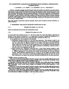
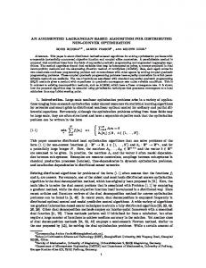
State

1 0.8 0.6 0.4 0.2 0 15 15

10 10 5

5 0

0 Ay-v-f

100 80 60 40 20 0 15 15

10 10 5

5 0

0

23

References 1. Barbu V., Optimal Control of Variational Inequalities, Research Notes in Mathematics, Pitman, Boston, Massachussets, Vol.100, 1984. 2. Mignot F. and Puel J.P., Optimal Control in Some Variational Inequalities , SIAM Journal on Control and Optimization, Vol. 22, pp.466-476,1984. 3. Zheng X. H., State Constrained Control Problems Governed by Variational Inequalities , SIAM Journal on Control and Optimization, Vol. 25, pp.1119-1144,1987. 4. Bergounioux M., Optimality Conditions for Optimal Control of the Obstacle Problem, to appear. 5. Bergounioux M., Optimality Conditions For Optimal control of Elliptic Problems Governed by Variational Inequalities : A Mathematical Programming Approach , Proceedings of the IFIP Conference on System Modelling and Optimization of Distributed Parameters with Applications to Engineering, Chapman and Hall, pp.123-131, 1996. 6. Bergounioux M., Optimal Control of Problems governed by Abstract Variational Inequalities with State Constraints, Preprint 96-15, Universite d'Orleans, Orleans, France, 1996. 7. Fortin M. and Glowinski R., Methodes de Lagrangien Augmente, Applications a la Resolution Numerique de Problemes aux Limites, Methodes Mathematiques de l'Informatique, Dunod, Paris,France, Vol.9, 1982. 8. Friedman A., Variational Principles and Free-Boundary Problems, Wiley, New York, 1982. 9. Bergounioux M. and Tiba D., General Optimality Conditions for Constrained Convex Control Problems, SIAM Journal on Control, Vol. 34, pp. 698-711, March 1996. 10. Bergounioux M., An Augmented Lagrangian Algorithm for Distributed Optimal Control Problems with State Constraints, Journal of Optimization Theory and Applications, Vol. 78, pp. 493-521, 1993. 11. Bergounioux M. and Kunisch K., Augmented Lagrangian Techniques for Elliptic State Constrained Optimal Control Problems, to appear. 12. Glowinski R. and Le Tallec P., Augmented Lagrangian and Operator-Splitting Methods in Nonlinear Mechanics, SIAM Studies in Applied Mathematics, Philadelphia, Pensylvania,1989.

24

13. Ito K. and Kunisch K., The Augmented Lagrangian Method for Equality and Inequality Constraints in Hilbert Spaces, Mathematical Programming, Vol.46, pp.341-360, 1990. 14. Malanowski K., Regularity of solutions in stability analysis of optimization and optimal control problems, Control and Cybernetics, Vol.23, pp.61-86, 1994. 15. Ito K. and Kunisch K., Augmented Lagrangian Methods for Nonsmooth Convex Optimization in Hilbert Spaces, Preprint, Berlin, Germany, 1994. 16. Bermudez A. and Saguez C., Optimal control of variational inequalities : Optimality conditions and numerical methods , Free Boundary Problems : Applications and Theory, Research Notes in Mathematics, Pitman, Boston, Vol.121, pp.478-487, 1988.

25