development and process automation of map generation. Front cover: the map ..... Egypt and Turkey and with Dr. Boujenane by email. The collaborators were ...
ICARDA
USE OF GIS TOOLS FOR THE INTEGRATION OF PRODUCTION ENVIRONMENT DESCRIPTORS OF ANIMAL GENETIC RESOURCES
E. De Pauw, B. Rischkowsky, A. Abou-Naga, H.R. Ansari-Renani, I. Boujenane, O. Gursoy
Final Report of Project “Practical Application of Production Environment Descriptors for Animal Genetic Resources – country case studies for sheep and goat breeds” (Letter of Agreement of FAO with ICARDA PR 43410) November 2011
1
ACKNOWLEDGEMENT The authors thank Ms. Beate Scherf of FAO for her effective coaching and monitoring throughout the duration of the project, as well as her colleagues at FAO for the valuable comments that have helped to improve the content of the report. Thanks are due to the efforts of the ICARDA GIS team, particularly Ms. Layal Atassi and Mr. Fawaz Tulaymat, for preparing the numerous high-quality maps, and to Mr. Jalal Omary, for the software development and process automation of map generation.
Front cover: the map shows similarity in the natural environment of parts of Europe, Africa and Asia with the distribution area of the Turkish Dagliç sheep breed.
i
TABLE OF CONTENTS 1. INTRODUCTION 2. METHODOLOGY 2.1. Selection of countries/breeds for the pilot study 2.2. Mapping the geographical distribution of the breeds 2.3. Obtaining additional management data 2.4. Characterization of breeds, distribution areas and management factors 2.4.1. Characterization of the selected breeds 2.4.2. Characterization of the distribution areas 2.4.2.1. Annual precipitation 2.4.2.2. Agro-climatic zones 2.4.2.3. Landforms 2.4.2.4. Land use/land cover 2.4.2.5. Agro-ecological zones 2.4.2.6. Soil management domains 2.5. Mapping adaptability zones for the breeds of the pilot countries 2.5.1. Data sources 2.5.2. Mapping climatic similarity 2.5.3. Mapping soil similarity 2.5.4. Mapping landform similarity 2.5.5. Mapping similarity in all evaluated factors 2.6. Comparison of DAD-IS spatial data with ICARDA data for breed areas 3. RESULTS 3.1. Characteristics of the selected breeds 3.1.1. Production systems and management 3.1.2. Environmental challenge and specific adaptations 3.1.3. Socioeconomic characteristics 3.2. Breed distribution areas 3.3. Environmental characteristics of the selected breed distribution areas 3.3.1. General 3.3.2. Agro-climatic zones 3.3.3. Soil management domains 3.3.4. Agro-ecological zones 3.3.5. Effect of input spatial data on characterization results 3.3.5.1. Comparison of CRU and ICARDA climate layers 3.3.5.2. Climates according to Köppen
3.4. Agricultural environments with high similarity to the selected breed distribution areas 4. DISCUSSION AND CONCLUSIONS 4.1. New approaches for improving the PEDS methodology 4.2. Limitations 4.2.1. Usefulness of the data collected from the questionnaires 4.2.2. Accessibility of country-level environmental datasets 4.3. New datasets for PEDS and DAD-IS REFERENCES
i
ANNEXES 1. Breed characterization data 2. Environmental characterization of breed distribution areas 3. Comparison of breed area characterizations using DAD-IS and ICARDA datasets 4. On-line (FTP: report, GIS data, Excel tables, maps, software) LIST OF TABLES Table 1. Number of sheep and goat breeds included in the study Table 2. Classes for the moisture regime Table 3. Classes for the winter type Table 4. Classes for the summer type Table 5. Conversion of FAO soil types into new soil management groups Table 6. Key attributes of selected breeds from Egypt Table 7. Key attributes of selected breeds from Iran Table 8. Key attributes of selected breeds from Morocco Table 9. Key attributes of selected breeds from Turkey Table 10.Number of sheep and goat breeds with special adaptive traits by country Table 11. Areas (km2) of the selected breeds Table 12.Agro-climatic zones of the breed distribution areas Table 13. Soil management domains of the breed distribution areas Table 14.Agro-ecological zones of the breed distribution areas Table 15. Levels of the Köppen classification for Iran used in the Peel et al.2007 and ICARDA layers Table 16. Anatolian Merino sheep: percent of each country in different environmental similarity classes Table 17. Characterization of sheep and goat breeds of Morocco Table 18. Characterization of sheep and goat breeds of Egypt Table 19. Characterization of sheep and goat breeds of Iran Table 20. Characterization of sheep and goat breeds of Turkey Table 21. Areas (%) in different precipitation classes in the sheep breed distribution areas of Egypt Table 22. Areas (%) in different precipitation classes in the goat breed distribution areas of Egypt Table 23. Areas (%) in different agro-climatic zones in the sheep breed distribution areas of Egypt Table 24. Areas (%) in different agro-climatic zones in the goat breed distribution areas of Egypt Table 25. Areas (%) in different landform classes in the sheep breed distribution areas of Egypt Table 26. Areas (%) in different landform classes in the goat breed distribution areas of Egypt Table 27. Areas (%) in different land use/land cover classes in the sheep breed distribution areas of Egypt Table 28. Areas (%) in different land use/land cover classes in the goat breed distribution areas of Egypt Table 29. Areas (%) in different soil management domains in the sheep breed distribution areas of Egypt Table 30. Areas (%) in different soil management domains in the goat breed distribution areas of Egypt Table 31. Areas (%) in different agro-ecological zones in the sheep breed distribution areas of Egypt Table 32. Areas (%) in different agro-ecological zones in the goat breed distribution areas of Egypt Table 33. Areas (%) in different precipitation classes in the sheep breed distribution areas of Iran Table 34. Areas (%) in different precipitation classes in the sheep breed distribution areas of Iran (2) Table 35. Areas (%) in different precipitation classes in the sheep breed distribution areas of Iran (3) Table 36. Areas (%) in different precipitation classes in the goat breed distribution areas of Iran Table 37. Areas (%) in different agro-climatic zones in the sheep breed distribution areas of Iran (1) Table 38. Areas (%) in different agro-climatic zones in the sheep breed distribution areas of Iran (2) Table 39. Areas (%) in different agro-climatic zones in the sheep breed distribution areas of Iran (3) Table 40. Areas (%) in different agro-climatic zones in the goat breed distribution areas of Iran ii
Table 41. Areas (%) in different landform classes in the sheep breed distribution areas of Iran (1) Table 42. Areas (%) in different landform classes in the sheep breed distribution areas of Iran (2) Table 43. Areas (%) in different landform classes in the sheep breed distribution areas of Iran (3) Table 44. Areas (%) in different landform classes in the goat breed distribution areas of Iran Table 45. Areas (%) in different land use/land cover classes in the sheep breed distribution areas of Iran (1) Table 46. Areas (%) in different land use/land cover classes in the sheep breed distribution areas of Iran (2) Table 47. Areas (%) in different land use/land cover classes in the sheep breed distribution areas of Iran (3) Table 48. Areas (%) in different land use/land cover classes in the goat breed distribution areas of Iran Table 49. Areas (%) in different soil management domains in the sheep breed distribution areas of Iran (1) Table 50. Areas (%) in different soil management domains in the sheep breed distribution areas of Iran (2) Table 51. Areas (%) in different soil management domains in the sheep breed distribution areas of Iran (3) Table 52 Areas (%) in different soil management domains in the goat breed distribution areas of Iran Table 53. Areas (%) in different agro-ecological zones in the sheep breed distribution areas of Iran (1) Table 54. Areas (%) in different agro-ecological zones in the sheep breed distribution areas of Iran (2) Table 55. Areas (%) in different agro-ecological zones in the sheep breed distribution areas of Iran (3) Table 56. Areas (%) in different agro-ecological zones in the goat breed distribution areas of Iran Table 57. Areas (%) in different annual precipitation classes in the sheep and goat breed distribution areas of Morocco Table 58. Areas (%) in different agro-climatic zones in the sheep and goat breed distribution areas of Morocco Table 59. Areas (%) in different landform classes in the sheep and goat breed distribution areas of Morocco Table 60. Areas (%) in different land use/land cover classes in the sheep and goat breed distribution areas of Morocco Table 61. Areas (%) in different soil management domains in the sheep and goat breed distribution areas of Morocco Table 62. Areas (%) in different agro-ecological zones in the sheep and goat breed distribution areas of Morocco Table 63. Areas (%) in different annual precipitation classes in the sheep breed distribution areas of Turkey (1) Table 64. Areas (%) in different annual precipitation classes in the sheep breed distribution areas of Turkey (2) Table 65. Areas (%) in different annual precipitation classes in the goat breed distribution areas of Turkey Table 66. Areas (%) in different agro-climatic zones in the sheep breed distribution areas of Turkey (1) Table 67. Areas (%) in different agro-climatic zones in the sheep breed distribution areas of Turkey (2) Table 68. Areas (%) in different agro-climatic zones in the goat breed distribution areas of Turkey Table 69. Areas (%) in different landform classes in the sheep breed distribution areas of Turkey (1) Table 70. Areas (%) in different landform classes in the sheep breed distribution areas of Turkey (2) Table 71. Areas (%) in different landform classes in the goat breed distribution areas of Turkey Table 72. Areas (%) in different land use/land cover classes in the sheep breed distribution areas of Turkey (1) iii
Table 73. Areas (%) in different land use/ land cover classes in the sheep breed distribution areas of Turkey (2) Table 74. Areas (%) in different land use/ land cover classes in the goat breed distribution areas of Turkey Table 75. Areas (%) in different soil management domains the sheep breed distribution areas of Turkey (1) Table 76. Areas (%) in different soil management domains in the sheep breed distribution areas of Turkey (2) Table 77. Areas (%) in different soil management domains in the goat breed distribution areas of Turkey Table 78. Areas (%) in different agro-ecological zones in the sheep breed distribution areas of Turkey (1) Table 79. Areas (%) in different agro-ecological zones in the sheep breed distribution areas of Turkey (2) Table 80. Areas (%) in different agro-ecological zones in the goat breed distribution areas of Turkey Table 81. Annual precipitation difference table between ICARDA and DAD-IS layers for the sheep areas in Egypt Table 82. Annual precipitation difference table between ICARDA and DAD-IS layers for the goat areas in Egypt Table 83. Maximum temperature difference table between ICARDA and DAD-IS layers for the sheep areas in Egypt Table 84. Maximum temperature difference table between ICARDA and DAD-IS layers for the goat areas in Egypt Table 85. Annual precipitation difference table between ICARDA and DAD-IS layers for the sheep areas in Iran (1) Table 86. Annual precipitation difference table between ICARDA and DAD-IS layers for the sheep areas in Iran (2) Table 87. Annual precipitation difference table between ICARDA and DAD-IS layers for the sheep areas in Iran (3) Table 88. Annual precipitation difference table between ICARDA and DAD-IS layers for the goat areas in Iran Table 89. Maximum temperature difference table between ICARDA and DAD-IS layers for the sheep areas in Iran (1) Table 90. Maximum temperature difference table between ICARDA and DAD-IS layers for the sheep areas in Iran (2) Table 91. Maximum temperature difference table between ICARDA and DAD-IS layers for the sheep areas in Iran (3) Table 92. Maximum temperature difference table between ICARDA and DAD-IS layers for the goat areas in Iran Table 93. Köppen class difference table between ICARDA and DAD-IS layers for the sheep areas in Iran (1) Table 94. Köppen class difference table between ICARDA and DAD-IS layers for the sheep areas in Iran (2) Table 95. Köppen class difference table between ICARDA and DAD-IS layers for the sheep areas in Iran (3) Table 96. Annual precipitation difference table between ICARDA and DAD-IS layers for the sheep and goat areas in Morocco Table 97. Maximum temperature difference table between ICARDA and DAD-IS layers for the sheep and goat areas in Morocco Table 98. Annual precipitation difference table between ICARDA and DAD-IS layers for the sheep areas in Turkey (1) iv
Table 99. Annual precipitation difference table between ICARDA and DAD-IS layers for the sheep areas in Turkey (2) Table 100. Annual precipitation difference table between ICARDA and DAD-IS layers for the goat areas in Turkey Table 101. Maximum temperature difference table between ICARDA and DAD-IS layers for the sheep areas in Turkey (1) Table 102. Maximum temperature difference table between ICARDA and DAD-IS layers for the sheep areas in Turkey (2) Table 103. Maximum temperature difference table between ICARDA and DAD-IS layers for the goat areas in Turkey LIST OF FIGURES Figure 1.Developing the Agro-climatic Zones framework Figure 2. Use of calibration factors to adjust sensitivity to a climatic parameter Figure 3. Assessing area similarity using two points along a gradient of precipitation (left) and temperature (right) Figure 4. Distribution of selected sheep breeds in Egypt Figure 5. Distribution of selected goat breeds in Egypt Figure 6. Distribution of selected sheep breeds in Iran (1) Figure 7. Distribution of selected sheep breeds in Iran (2) Figure 8. Distribution of selected goat breeds in Iran Figure 9. Distribution of selected sheep breeds in Morocco Figure 10. Distribution of selected goat breeds in Morocco Figure 11. Distribution of selected sheep breeds in Turkey (1) Figure 12. Distribution of selected sheep breeds in Turkey (2) Figure 13. Distribution of selected goat breeds in Turkey Figure 14. Correlations between pixels in each thematic class of the maximum temperature of the warmest month for sheep breeds and goat breeds of Egypt Figure15. Correlation between the percentages in each thematic class of the annual precipitation for sheep breeds of Turkey Figure 16. Mean annual precipitation in Turkey (CRU layer) Figure 17. Mean annual precipitation in Turkey (ICARDA layer) Figure 18. Maximum temperature of the warmest month in Egypt (CRU layer) Figure 19. Maximum temperature of the warmest month in Egypt (ICARDA layer) Figure 20. Minimum temperature of the coldest month in Morocco (CRU layer) Figure 21. Minimum temperature of the coldest month in Morocco (ICARDA layer) Figure 22. Köppen climatic zones in Iran (Peel et al., 2007) Figure 23. Köppen climatic zones in Iran (ICARDA layer) Figure 24. Global temperature similarity with the breed distribution area of Dagliç sheep, Turkey Figure 25. Global precipitation similarity with the breed distribution area of Dagliç sheep, Turkey Figure 26. Global landform similarity with the breed distribution area of Dagliç sheep, Turkey Figure 27. Global soil pattern similarity with the breed distribution area of Dagliç sheep, Turkey Figure 28. Global similarity in climate, landforms and soils with the breed distribution area of Dagliç sheep, Turkey
v
1. INTRODUCTION Improved understanding of the adaptation of livestock breeds to their production environments is important for many decisions in the field of animal genetic resources (AnGR) management. However, adaptation is complex and difficult to measure. One approach is to characterize adaptation indirectly by describing the production environments in which a breed has been kept over time, and to which it has probably become adapted. Comprehensive and comparable descriptions of the production environments in which animals are kept are also vital to make meaningful evaluations of performance data and to enable comparative analysis of the performance of different breeds. To address the requirement of defining production environments, FAO has proposed that a recognized set of “production environment descriptors” (PEDs) should be established and used throughout the world as a common framework for describing breeds’ production environments. An expert workshop on Production Environment Descriptors for Animal Genetic Resources (FAO/WAAP, 2008), held in 2008 (shorthand: PEDS Workshop) completed the framework and proposed a set of PEDS. The workshop concluded that descriptors for the natural environment can be best obtained by mapping the location of the breed and linking this to existing GIS-based datasets; and that the management environment descriptors should be collected by a standard set of questions about each breed describing the management conditions in which the breed is kept. Accordingly questionnaires were developed to collect relevant data on management, production systems and breed characteristics. Based on the outcomes of the workshop the FAO team has been developing a PEDs module for the Domestic Animal Diversity Information System (DAD-IS; http://dad.fao.org/) hosted by FAO. DAD-IS is a global information system and serves as a communication and information tool for the management of animal genetic resources (AnGR). It provides the user with searchable databases of breed-related information and images, management tools, and a library of references, links and contacts of Regional and National Coordinators for the Management of AnGR. It provides countries with a secure means to control the entry, updating and accessing of their national data, a forum for exchange of ideas and techniques; country, regional and global contacts; and a repository for documents related to the management of AnGR. The new PEDS module in DAD-IS is supposed to allow the National Coordinators (NCs)1to enter the description of the production environments and special characteristics related to adaptation for the breeds in their countries. A mapping tool will allow them to enter spatial data. There are several challenges to the proposed approach: the degree of knowledge on production environments to be expected from National Coordinators or other national AnGR experts in the countries; ease of collecting information on breed distributions of all species; availability and accessibility of GIS referenced datasets on the natural environment once the breed distribution has been captured. To address these challenges and to practically test the PEDs approach, FAO and ICARDA initiated a pilot study in 2010 with sheep and goat breeds in four countries. The specific objectives of the projects included: 1
NCs are appointed officially by the Ministry of Agriculture and form FAO’s international network for the management of AnGR.
1
developing a data capturing tool following the questionnaire included in the report of the PEDS workshop and transferring the data collected for sheep and goat breeds in the four selected countries developing methodologies such as similarity mapping and agro-ecological zoning (ICARDA methodology) for aggregating the PEDs and arrive at predictions of adaptive traits of breeds comparing the analytic results from the GIS layers describing the natural environment currently being made available at global scale for DAD-IS with the GIS layers available at ICARDA.
A new DAD-IS module enabling capturing of data related to production environments in which certain portions of breed populations are kept was supposed to be finalized and launched by FAO in mid 2010 and then tested and used by ICARDA. Due to a delay in the finalization and launching of the new module by FAO, ICARDA was unable to collect and capture the pilot data using the DAD-IS module as agreed. Instead, FAO requested ICARDA to develop a data capturing system in order to implement the other elements of the LoA. Thus the final agreed outputs from this project were: • improved GIS data of goat and sheep breed distribution for four countries, namely Egypt, Iran, Morocco and Turkey, entered in DAD-IS, • a methodology for aggregating individual production environment descriptors to enable automated overviews of AnGR diversity by production environment in DAD-IS, • a comparison of results from some environmental spatial datasets to be used in DAD-IS with higherresolution spatial data available at ICARDA. • a final report including the breed distribution maps for the above named countries and maps of aggregated PEDs at country and at global scale.
2
2. METHODOLOGY 2.1. SELECTION OF COUNTRIES/BREEDS FOR THE PILOT STUDY Egypt, Iran, Morocco, and Turkey were selected as pilot countries they contain a diverse mix of goat and sheep breeds and of agro-ecological zones in non-tropical dry areas. Furthermore, these countries had been included in the characterization of sheep and goat breeds carried out by ICARDA in West Asia and North Africa (Iñiguez, 2005). For our study we contacted NARs scientists in the four countries that had collaborated with ICARDA in the previous characterization studies. The collaborators for our study were: Egypt: Dr. Adel Abou-Naga2, Animal Production Science Research Institute, Cairo Iran: Dr. M.A. Abbasi and Dr. Hamid Reza Ansari-Renani3, Animal Science Research Institute, Karaj Morocco: Dr. Ismail Boujenane4, Institut Agronomique et Vétérinaire Hassan II, Rabat Turkey: Prof. Dr. OktayGursoy, Çukurova University, Adana The project was explained and discussed in detail with the national collaborators during visits in Iran, Egypt and Turkey and with Dr. Boujenane by email. The collaborators were informed that at the end of the project all information would be shared with FAO and the National Coordinators. The partners from Turkey and Morocco were provided with the contact details of the National Coordinators. Then the lists of local sheep and goat breeds were agreed upon for the four countries. Clearly distinct local/indigenous breeds or already well-established crossbred/synthetic breeds such as the Anatolian Merino in Turkey that have been adopted and are spread among producers were included. International trans-boundary breeds present in the countries were excluded because their distribution is not determined by adaptation to the natural environment but rather by the presence of more intensive production systems or a research/development program. Thus, mapping their distribution would not have added value to this study .An exception was made for the Awassi breed because of its high regional importance. In total 61 sheep and 24 goat breeds were included (Table 1). Table 1. Number of sheep and goat breeds included in the study Species
Morocco
Egypt
Turkey
Iran
Total
Sheep breeds
6*
8
20
27
61
Goat breeds
4
7
6
7
24
10
15
26
34
85
Total
*For 5 sheep breeds in addition to the current geographical distribution their origins were mapped.
A short description of the included breeds was provided in the Annex tables of the first progress report. In April 2011 the breeds included in the current study were compared with the breed entries (inventory) 2
Dr.Abou Naga was officially nominated as National Coordinator for AnGR in Egypt end of 2010. Dr.Abbasi was appointed by Dr.Kamali, the NC of Iran, to represent him in this project, but the data and maps were submitted by Dr. Hamid Reza Ansari-Renani, another scientist from the same institute. 4 Dr.Boujenane and Prof.Gursoy were authors of the respective country book chapters in the Characterization of small ruminant breeds in West Asia and North Africa (Iñiguez, 2005). 3
3
in DAD-IS; the direct link to the breed entry in DAD-IS IS was added to the tables and sent to FAO. The comparison of breeds listed for this project with DAD-IS entries was based on ICARDA's book series on small ruminant (SR) breed characterization and the knowledge of our collaborators. It revealed that a number of breed entries in DAD-IS should be corrected and some removed: for some breeds there was no other information besides the names in DAD-IS and they were not known to our collaborators. They are probably varieties of another breed with no clear description; some breeds are listed twice in DAD-IS under slightly different names but are definitely the same breeds. In the case of Egypt and Iran the information was fed back to the NCs. It is proposed that FAO would share the DAD-IS tables in which we marked the questionable breeds with the National Coordinators in Morocco and Turkey. In particular, Morocco would need a serious update as there are many breeds listed in DAD-IS without any information and it is not clear if these breeds still exist or have ever been present in the country. Maybe here and in other countries information from the country report was added that was not relevant or accurate.
2.2. MAPPING THE GEOGRAPHICAL DISTRIBUTION OF THE BREEDS FAO’s mapping tool was not ready in time to be used and tested in this project. Instead ICARDA’s GIS Unit scanned detailed road maps of the countries and sent them electronically and as hard copies to the collaborators. The collaborator from Iran used the electronic copy of the map and a paint program to draw the breed distributions and sent us the maps in electronic format. The other three collaborators preferred to draw the boundaries of the breed distributions in the hard copies of the maps and sent the hard copies back to ICARDA. Prof. Gursoy actually visited ICARDA in December 2010 and explained the borders of breed distribution for Turkey that he had demarcated on the maps directly to the ICARDA scientists. To illustrate the process of defining the breed domains, an example of a ‘raw’ breed distribution map (for sheep in Western Turkey) was sent to FAO together with the first progress report. In Egypt the breed distributions were mapped by the NC using the boundaries of the Egyptian agroecological zones in which they occur. The breed distribution maps for the four countries were digitized and converted into ESRI shapefiles and sent to FAO on a DVD. The digital distribution maps prepared by GISU were validated with the Egyptian collaborators during a meeting in April 2011 and the maps corrected accordingly by GISU. Final maps of the individual breed distributions were prepared and are included on the DVD as Annex 3. Consolidated country maps for sheep and goat breeds are presented in figures 4 to 13.
2.3. OBTAINING ADDITIONAL MANAGEMENT DATA As FAO’s data entry mask in DAD-IS was not ready, the collaborators filled the questionnaires (word documents) as developed by the PEDS workshop. For each breed two questionnaires/worksheets, namely Annex 4a. Production environment descriptors and Annex 4b: Worksheet for describing breeds’ special qualities, were filled. The information from the Word documents was transferred to an Excel sheet to allow an analysis of the available data. The Word documents are to be sent together with the maps to FAO. For Iran and Egypt this information could be directly entered into DAD-IS as our collaborators would have access to the country database in DAD-IS. 4
A major difficulty for all collaborators was to enter the required information on disease challenges and treatments as the collaborators are breeders. This may also be the case for the National Coordinators in other countries. To overcome this hurdle it would be useful to generate digital maps of disease prevalence (compare 4.2.1).
2.4. CHARACTERIZATION OF BREEDS, DISTRIBUTION AREAS AND MANAGEMENT FACTORS 2.4.1. Characterization of the selected breeds A complete characterization of the selected breeds was carried out following the PEDS framework using indicators belonging to the following thematic areas:
Length of time that the breed has been in its production environment Climate modifiers Feed and water availability and management Contribution by each feed type of dry matter fed to the animals in the vegetation period and outside the vegetation period, or throughout the year in case there is no specific vegetation period Main uses and roles of the breed in this production environment Breed characteristics relevant to climate Breed characteristics relevant to terrain Breed tolerance relevant to feed and water availability Special adaptation features Specific quality of products
The full database compiled on breed characterization in accordance with the PEDS framework is included as an Excel spreadsheet. 2.4.2. Characterization of the distribution areas Prior to the implementation of the PEDS module, DAD-IS did not contain a template for the detailed description of the natural environment. Lack of a structured description template forced the National Coordinators or their representatives into very general non-standardized descriptions or narratives of the natural environment. The PEDS module currently contains descriptors for the natural environment related to : climate (temperature, precipitation, relative humidity, wind, daylength, solar radiation) terrain (altitude, slope, soil pH, surface conditions) diseases, parasites and other animal health threats These descriptors are not yet available for data-entry in DAD-IS, but once they are, may help to characterize the breed natural environments more accurately. A disadvantage of these descriptors is that they are basically single-value descriptors, in the sense that an average attribute value is to be assigned for the entire breed area. Therefore the spatial variability within the breed area, which can be very considerable, particularly if the breed area is very large and contains strong elevation or climatic gradients, is not taken into consideration. Yet the variability in the resource base within a breed area in space and time may be key to its adaptation. Moreover there is a high risk of errors in these averages, as 5
true area averages can only be obtained from knowledge of the attribute values in individual locations. It is precisely in this respect that the use of spatial datasets in conjunction with GIS tools may allow more accurate assessments of the natural environments, particularly if up-to-date and reliable national databases are available and accessible. Having no access to recent, quality-controlled national data the following international data sources were used for the characterization of the breed distribution areas in the four countries: 1) For climate: De Pauw, E. 2008. Climatic and Soil Datasets for the ICARDA Wheat Genetic Resource Collections of the Eurasia Region. Explanatory Notes. ICARDA GIS Unit, Aleppo, Syria.68 pages. (http://geonet.icarda.cgiar.org/geonetwork/data/regional/GRU_NetBlotch/Doc/Report_NetBlotch.pdf). 2) For terrain: SRTM30 Digital Elevation Model (http://topex.ucsd.edu/WWW_html/srtm30_plus.html) 3) For soils: FAO-UNESCO.1995. The Digital Soil Map of the World and Derived Soil Properties. Land and Water Digital Media Series 1. FAO, Rome, CD-ROM. 4) For land use/land cover: D. Celis, E. De Pauw and R. Geerken. 2007. Assessment of land cover/ land use in the CWANA region using AVHRR imagery and agro-climatic data. Part 1. Land Cover/Land Use - base year 1993. International Center for Agricultural Research in the Dry Areas (ICARDA), Aleppo, Syria, vi+ 54 pp. ISBN 92-9127-192-4 5) For agro-ecological zones: E. De Pauw. 2010. Agro-ecological zoning of the CWANA region. In A. El-Beltagy and M.C. Saxena (Eds.).Sustainable Development in Drylands – Meeting the Challenge of Global Climate Change. Proceedings of the Ninth International Conference on Development of Drylands, 7-10 November 2008, pp. 335-348, International Drylands Development Commission, ICARDA. Map available for viewing on the ICARDA web site (http://www.icarda.cgiar.org/hps_11-0327_WhatCanGrow.htm) From these datasets the following attributes were derived for the characterization of the production environments of the selected breeds: Annual precipitation Agro-climatic zones Landforms Land use/land cover Soil Management domains Agro-ecological zones Characterization in terms of the above themes was done by classification of each attribute into relevant classes and by tabulating the proportion of each class in each breed distribution area. The latter were obtained through the Zonal Histogram function of the Spatial Analyst module in ArcGIS software.
6
The description and classification of the characterization attributes of the breed distribution areas is provided in the following sections. 2.4.2.1. Annual precipitation This is a GIS raster layer with spatial resolution of 30 arc-seconds (0.0083333 decimal degrees, or nearly 1 km in N-S direction) obtained by spatial interpolation of station-based climatic data. The interpolation method was the ‘thin-plate smoothing spline’ method of Hutchinson (1995), as implemented in the ANUSPLIN software (Hutchinson, 2000). The Hutchinson method is a smoothing interpolation technique that is guided by topography: the limited station precipitation data are extended across the entire grid by correlations with elevation. The latter was input to the model in the form of a DEM ASCII grid file. The DEM used to generate the climate surfaces was the SRTM30 DEM with 30 arc-second (approximately 1 km) resolution. The precipitation data are annual averages for different time periods, but with a minimum of 20 years in the case of precipitation. The main sources were international, such as the Food and Agriculture Organization of the United Nations and the National Climate Data Center of the US (NCDC). For Iran the data came mostly from national archives. 2.4.2.2. Agro-climatic zones The agro-climatic zones are combinations of GIS raster layers related to moisture regime, and winter and summer temperature regimes, in accordance with the criteria and class thresholds as implemented in the UNESCO classification system for arid regions (UNESCO, 1979). The classes are shown in Tables 13. Table 2. Classes for the moisture regime Moisture regime Aridity index
Hyper-arid (HA) 1
Table 3. Classes for the winter type Winter type Mean temp. coldest month
Warm (W) > 20°C
Mild (M) > 10°C
Cool (C) > 0°C
Cold (K) ≤ 0°C
Warm (W) > 20°C
Mild (M) > 10°C
Cool (C) ≤ 10°C
Table 4. Classes for the summer type Summer type Mean temp. warmest month
Very warm (VW) > 30°C
In this classification system the moisture regime is determined by the ratio of annual rainfall over annual potential evapotranspiration (also referred to as aridity index), calculated according to the Penmanmethod (Doorenbos and Pruitt, 1984).The potential evapotranspiration (PET) is a measure of the atmospheric water demand for a grass cover (and for crops by including crop coefficients).
7
The Aridity Index provides a waterbalance in its most elementary form (on annual basis) and takes account of higher moisture demand in hot climates, as well as differences in the effectiveness of precipitation for growth cycles that include a cold period versus those that do not (Table 2). The winter type is determined by the mean temperature of the coldest month (Table 3). The summer type is determined by the mean temperature of the warmest month (Table 4). The UNESCO system is basically open-ended and any particular climate can be described by the three attributes, moisture regime, winter type and summer type. Despite its apparent simplicity the UNESCO system is capable of capturing the key characteristics of an agricultural climate of relevance for livestock: degree of aridity and temperature conditions in the warmest and coldest month of the year. For example, the climate SA-C-VW is characterized by a semi-arid moisture regime, a cool winter type and very warm summer type.
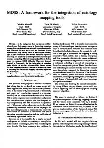
Figure 1. Developing the Agro-climatic Zones framework (Tp: temperature)
Figure 1 outlines the combination of basic and derived climatic surfaces used to generate the Agroclimatic Zones. 2.4.2.3. Landforms The most important attributes of topography relevant to livestock are the elevation and the slope. Due to the lapse of air temperature that takes place with increasing altitude, the effect of absolute elevation is basically a temperature effect, which is already accounted by the climatic classification explained in section 2.4.2.2. The slope obviously presents an accessibility effect that can be quantified using a highresolution digital elevation model, for example by the proportions of a breed area in different slope classes. However, to get an overview over the large areas that most breeds occupy, a simple classification of landforms appears adequate. Based on the SRTM30 digital elevation model (spatial resolution: 30 arc-seconds, 0.0083333 decimal degrees, or nearly 1 km in N-S direction) simplified landform classes were obtained using the following rules: 8
Plains: maximum elevation difference between neighboring pixels 0-50 m Hills: maximum elevation difference between neighboring pixels 50-300 m Mountains: maximum elevation difference between neighboring pixels > 300 m The maximum elevation difference between neighboring pixels was calculated using the Range function in the Spatial Analyst module of Arctic software with subsequent classification. 2.4.2.4. Land use/land cover Land use/land cover data for the breed distribution areas were extracted from the regional Land Use/Land Cover Map prepared by Celis et al. (2007) for the base year 1993. This is not the most up-todate map in the public domain, but probably more reliable than other land cover maps from international sources, as it contains a limited number of classes and has been given considerable ground truthing: barren/sparsely vegetated irrigated crops rainfed crops rangelands forests other land uses/cover type (mainly urban, water bodies) The distinction between rainfed and irrigated crops was considered relevant for livestock as irrigated areas usually produce higher yields, biomass and crop residues than rainfed areas, which are partially or entirely retained for livestock use. The spatial resolution of this thematic layer is also 30 arc-seconds, or about 1 km in N-S direction. 2.4.2.5. Agro-ecological zones Agro-ecological zones (AEZ) are the integrated spatial entities that emerge by the overlaying of agroclimatic zones, landforms, land use/land cover classes and soil patterns. The agro-ecological zones were generated by the following 6-step procedure: Converting point climatic data into basic climatic ‘surfaces’ through spatial interpolation; Generating a spatial framework of agro-climatic zones (ACZ) by combining the basic climatic surfaces into more integrated variables that provide a synthesis of climate conditions; Generating a spatial framework of land systems, which are integrated land-based mapping units, created by the combinations of major land use/land cover, landforms and soil categories; Integrating the frameworks for agro-climatic zones and land systems by overlaying in GIS; Removing redundancies, inconsistencies, and spurious mapping units generated by the overlaying process; Characterizing the AEZ in terms of other relevant themes (e.g. population density, land degradation, length of growing period etc.). The full procedure and data sources are described by De Pauw (2010). In order to avoid unnecessary complexity, in the current study we used as agro-ecological zones the integrated units formed by the overlaying of agro-climatic zones, landforms and land use/land cover, as described in the previous sections. To define the AEZ in terms of land use/land cover, a further simplification was done, using only 3 classes (irrigated crops, rainfed crops and non-agricultural land use). The latter class is a very diverse one, as it may contain grasslands, open or closed shrublands as well as barren/sparsely vegetated land. However, the regrouping of the land use/land cover classes into broader classes avoids repeating what is already known from the land use/land cover characterization, as described in section 2.4.2.1.
9
Section 3.3.3 contains the list of AEZs that occur in the breed distribution areas, as well as their short descriptions. 2.4.2.6. Soil management domains In the PEDS description module, soil pH is listed as a terrain attribute. Whereas certain soil characteristics (e.g. stoniness, sandy texture, wetness) undoubtedly influence terrain and its accessibility, these and other soil features (e.g. strong acidity, salinity, sodicity, flooding, water logging) may also act as proxies for vegetation communities. Thus soils and their management properties may acquire implicit or explicit significance in terms of the vegetation communities they support, with their own characteristics of palatability and nutrient status, or the physical or chemical constraints they impose on plant development. Soil management domains can be defined as combinations of soil types that have been merged into broader groupings that are relevant to such key management properties. The soil management domains were defined and mapped as part of an ICARDA project on agroecological zoning of the CWANA region (covering North Africa, the Horn of Africa, West and Central Asia) and the methodology is described by De Pauw (2010). Using the FAO Soil Map of the World (FAO, 1995) as data source, it was found that within the CWANA region 1047 soil associations occur, as determined by varying combinations of 112 FAO soil types. Reducing this vast variability by regrouping was necessary in order to establish ecosystems that were not over-fragmented. This generalization was done in two steps: 1) regrouping the FAO soil types into broader classes that are relevant to their general management properties (‘soil management groups’) 2) mapping the major combinations of these soil management groups (‘soil management domains’) The 126 FAO soil units were reduced to 13 soil management groups as indicated in Table 5. Table 5. Conversion of FAO soil types into new soil management groups SMG
Soil Management Group
FAO soil types (Legend Soil Map of the World, 1974)
G1
Agricultural soils
B, Bc, Bd, Be, Bf, Bh, Bk, Bv, C, Cg, Ch, Ck, Cl, De, H, Hc, Hh, Hl, K, Kh, Kk, Kl, L, La, Lc, Lf, Lk, Lo, Lp, Lv, Mo, Nd, Ne, Nh, T, Th, Tm, To, V, Vc, Vp
G2
Soils of wetlands, poorly drained areas and floodplains Sandy soils Sodic and saline soils Rock outcrops and shallow soils Semi-desert soils Desert soils Non-agricultural soils Soils with high acidity and/or low nutrient status Glaciers Mobile sands Salt flats Water bodies
Ag,Bg, Dg, G, Gc, Gd, Ge, Gh, Gm, Gp, Hg, J, Jc, Jd, Je, Jt, Lg, Mg, O, Od, Oe, Ox, Pg Qa, Qc, Qf, Ql, Q S, Sg, Sm, So, Ws, Z, Zg, Zo, Zt, Zm E, I, RK, U X, Xh, Xk, Xl, Xy Y, Yh, Yk, Yl, Yt, Yy Bx, Gx, R, Rc, Rd, Re, Rx, Tv,Wd, We, Wm Af, Ah, Ao, Ap, D, Dd, Fa, Fh, Fo, Fp, Fr, Fx, P, Ph, Pl, Po, Pp GL DS ST WR
G3 G4 G5 G6 G7 G8 G9 G10 G11 G12 G13
10
Using these new soil groupings the units of the Soil Map of the World were converted by reclassifying the 1047 FAO soil associations into 60 Soil Management Domains (SMD). The SMDs are thus regroupings of the FAO soil associations on the basis of the main management properties of the soils, through combinations of the main soil management groups. Section 3.3.4 contains the list of SMDs that occur in the breed distribution areas, as well as their short descriptions.
2.5. MAPPING ADAPTABILITY ZONES FOR THE BREEDS OF THE PILOT COUNTRIES The key concept for assessing to which environments the breeds of the pilot countries could be adapted is similarity in physical environments with the breed distribution areas. Thus the breed distribution maps and their associated physical characteristics are the basis for identifying areas outside the current breed areas where the breeds in question are likely to be adapted. In this study we assessed similarity at the global scale at a spatial resolution of 30 arc-seconds (about 1 km in N-S direction). The methodology for assessing similarity takes into consideration the more permanent characteristics of the biophysical environment: climate, topography and soils. It did not include land use/land cover as this is often a fairly dynamic attribute and, moreover, current global land use/land cover maps were not considered of adequate accuracy for this exercise to be meaningful. In similarity analysis, the value of a parameter or index at one location (the ‘match’ location) is compared with other (‘target’) locations in order to quantify the degree of similarity. In this particular case the thematic pattern in each one of the breed distribution areas, as drawn by the national collaborators, has been used as representing the match location. The target area is the entire land area of the earth with the exception of Antarctica, Greenland, and other glaciated areas. Excluded from the similarity analysis were also the hyper-arid areas, or true deserts (i.e. with an annual aridity index below 0.03). These areas were simply excluded by masking them. The similarity mapping was done in different stages: similarity in temperature, in precipitation, landforms and soils were mapped separately using individual similarity indices and the thematic similarity indices were then combined into an overall similarity index for the natural environment. The methods for similarity mapping of temperature and precipitation are essentially the same as those used for a regional study of the Karkhe River Basin in Iran (De Pauw et al., 2008), with this difference that for the current study new software has been developed that makes global assessments feasible. The methods for assessing soil and landform similarity are new and have been applied for the first time in this study. Several computer programs were developed to automate the process, which are included on the DVD. In the course of the study a ‘striped map’ software bug was discovered and corrected. 2.5.1. Data sources The following spatial data sources were used as input to the similarity mapping at the global scale: 1) For temperature similarity: Hijmans, R.J., S.E. Cameron, J.L. Parra, P.G. Jones and A. Jarvis, 2005. Very high resolution interpolated climate surfaces for global land areas. Int. J. Climatology 25: 1965-1978 (http://worldclim.org/current)
11
2) For precipitation similarity: Hijmans, R.J., S.E. Cameron, J.L. Parra, P.G. Jones and A. Jarvis, 2005. Very high resolution interpolated climate surfaces for global land areas. Int. J. Climatology 25: 1965-1978 (http://worldclim.org/current) De Pauw, E. 2008. Climatic and Soil Datasets for the ICARDA Wheat Genetic Resource Collections of the Eurasia Region. Explanatory Notes. ICARDA GIS Unit, Aleppo, Syria.68 pages. (http://geonet.icarda.cgiar.org/geonetwork/data/regional/GRU_NetBlotch/Doc/Report_NetBlotch.pdf). 3) For landform similarity: SRTM30 Digital Elevation Model (http://topex.ucsd.edu/WWW_html/srtm30_plus.html) 4) For soil pattern similarity: FAO-UNESCO.1995. The Digital Soil Map of the World and Derived Soil Properties. Land and Water Digital Media Series 1. FAO, Rome, CD-ROM. 5) For similarity in natural environment: all of above data sources 2.5.2. Mapping climatic similarity The model used to assess climatic similarity is the combination of two distance functions, one for the temperature and another one for precipitation: (Eq.1)
S Min( I1( t ) , I 2 ( p ) )
with Min: the lowest of the two values The functions I1 and I2 are similarity indices for respectively air temperature and precipitation. These functions draw inspiration from the ‘Match Index’ concept developed in the CLIMEX software (Sutherst, 1999). They model the drop in similarity under increasing dissimilarity for air temperature t and precipitation p , respectively, as (Eq.2)
I1 e
t t
and
I2 e
p 10 p
with t [OC-1]and p [mm-1]user-defined calibration constants (Fig. 2). The assessment of similarity can be fine-tuned by user-defined calibration constants. Calibration constants determine the form of similarity decay functions (Fig.2), which model the drop in similarity under increasing difference in precipitation or temperature, and are user-selected. The role of the calibration constant is thus to adjust the sensitivity of the similarity index in terms of what the user expects as reasonable measures of quantified differences in the patterns of temperature or precipitation between the breed areas and the target locations. In this study the calibration factor for air temperature t was empirically set to 7.0, which corresponds to a drop in similarity by 20% under t = 2OC and of about 50% under t = 5OC. The calibration factor for precipitation pwas set to 3.0, which corresponds to a drop in similarity of 50% under p = 20 mm and of about 80% under p = 50 mm.
12
Δt Δp Figure 2. Use of calibration factors to adjust sensitivity to a climatic parameter
Climatic similarity is assessed on the full precipitation and temperature record. Twelve monthly values of average temperature and total precipitation are used. Similarity is quantified by the sum of squared distances between the parameter values of the match and each target location, using a scale of 0 (or 0%, totally dissimilar) to 1 (or 100%, totally similar). In order to avoid artificial dissimilarity due to different timing of growing periods (e.g. when comparing climates in different hemispheres), the temperature curves of the match and target locations are aligned first in such a way that the timing of the minimum and maximum temperatures has a maximum overlap. Data input was in the form of climatic grids (12 mean monthly precipitation and average temperature surfaces). To assess similarity, grids were used with SRTM30-DEM resolution (30 arc-second; 1 km). The dissimilarity in temperature t was computed as follows (De Pauw, 2002): 12
(Eq. 3)
t
t i 1
Ti
2
is
,
12
wherei is month number, t is mean monthly air temperature in the target point, T is mean monthly air temperature in the matching point (OC), s is a phase shift in month numbering. The phase shift minimizes the deviation in temperature between match and target location that could result from differences in geographical location and latitude. It is particularly important at the global scale as it allows to compare locations in both the northern and southern hemisphere by synchronizing the seasonal temperature pattern. The phase shift was obtained by shifting the temperature array until the covariance:
13
12
(Eq.4)
Cov(Tm, T ) (Tmi Tm ) (Ti T ) i 1
reaches a maximum. The highest possible phase is 11. The co-variance is very sensitive to small differences in monthly temperature between different locations and its use could, under certain conditions, produce in some areas a phase that is different from the one in its immediate surroundings in what is otherwise a climatically homogeneous region, leading to noisy patterns. To avoid that a generalization procedure is undertaken in the GIS software on the phase shift layer, which in ArcGIS 10 software can be described under the following steps: the Shift FLT-file is converted to raster the continuous floating point raster is converted to integer raster the FocalStats procedure is run twice with the settings Rectangular neighborhood (5x5) and Majority statistic the Boundary Clean procedure is run with sorting technique Descend a global Land Mask is used to extract the final generalized Shift layer Once the phase shift (s) is established, it was applied to calculate the dissimilarity in precipitation pattern (p): 12
(Eq. 5)
p
p i 1
is
Pi
2
,
12
where p is monthly precipitation in each target point, P monthly precipitation in the match point. The above formulas apply for a similarity assessment based on a point to point comparison. However, breed distribution areas, particularly large ones, may contain a range of precipitation and temperature conditions. To ensure that the internal climatic variations did not exaggerate the dissimilarity that may arise by taking only one point inside the breed area, the precipitation and temperature conditions in two points were considered, that represent a minimum and a maximum value (Fig.3).
Figure 3. Assessing area similarity using two points along a gradient of precipitation (left) and temperature (right)
14
These values were obtained by sorting all values of mean annual precipitation and temperature in the specific breed area and retaining the 1stand 9thdecile values. A computer program Extremes Excluder was developed for filtering out extreme values and identifying the 1st and 9th decile values. These values were then used to identify two locations for the precipitation gradient and two locations for the temperature gradient representing about 80% of the climatic conditions inside the breed area. If a monthly temperature value for the target location was between the monthly temperature values of the two match locations, the dissimilarity (Eq.3) for that month was set to zero. If higher than the highest of the two match location values, the dissimilarity was calculated between the target location and the highest of the two match location values. If lower than the lowest of the two match location values, the dissimilarity was calculated between the target location and the lowest of the two match location values. The same procedure was adopted for calculating the monthly dissimilarity for precipitation (Eq. 5). As mentioned before, to ensure that the similarity index for production zones with low precipitation does not lead to a misleading impression of high similarity with deserts, hyper-arid areas in which no sheep or goats are sustainable except in oases, have been masked. 2.5.3. Mapping soil similarity Soil similarity was assessed by comparing the composition of the soil association within the breed distribution areas with the soil composition of each land pixel. The soil composition of both the breed distribution areas and areas outside was obtained from the Digital Soil Map of the World (1995) using the soil classification established by FAO for this map (1974). As the legend for this map is a very complex one, containing more than 100 classes, the soils have been regrouped into broad soil management groups, which have similar properties in terms of soil management. These soil management groups, as well as the FAO soil classes they contain, are shown in Table 5. For more details on the symbols and definitions of the FAO soil types is referred to the Legend of the Soil Map of the World (FAO, 1974). Soil similarity was evaluated by applying the Sørensen similarity index to the management groups (G1, G2 ... G13) in accordance with the following steps: 1. If G1 is not present in both the breed distribution area and in the target pixel, no similarity index is calculated. 2. If G1 is present in the breed distribution area but not in the target pixel, or vice versa, the similarity index is zero. 3. In all other cases the similarity index for soil management group G1 is calculated as:
with
Min: the lowest value of the two %G1d: proportion (%) of SMG G1 in the soil composition of the breed distribution area %G1t: proportion (%) of SMG G1 in the soil composition of the target pixel 4. Steps 1-3 are repeated for soil management groups G2, G3 ... G13. 5. The total soil similarity is calculated as a weighted average of the similarity indices for each soil management group as follows:
15
with
%Gi,d: proportion (%) of SMG Gi in the soil composition of the breed distribution area
2.5.4. Mapping landform similarity Landforms were grouped into three classes based on the concept of ‘relief intensity’. ‘Relief intensity’ is obtained from the SRTM30 DEM dataset and is derived from the maximum elevation difference between two neighbouring pixels. The three relief intensity classes are:
L1: Plains; relief intensity 0-50 m L2: Hills; relief intensity 50-300 m L3: Mountains; relief intensity >300 m
For each breed distribution area the landform composition was recorded in terms of percentage plains (%L1), hills (%L2) and mountains (%L3). The procedure for assessing landform similarity is very similar to the one used to assess soil similarity: by comparing the landform composition within the breed distribution areas with the landform of each land pixel, with the only difference that in the latter the landform is homogeneous (100% L1 or 100% L2 or 100% L3). The rules are thus: 1. If L1 is not present in both the breed distribution area and in the target pixel, no similarity index is calculated. 2. If L1 is present in the breed distribution area but not in the target pixel, or vice versa, the similarity index is zero. 3. In all other cases the similarity index for landform L1 is calculated as: %𝐿1𝑑 ∗ 2 𝑆𝑖𝑚𝐿1 = %𝐿1𝑑 + 100 with %L1d: proportion (%) of landform L1 in the landform composition of the breed distribution area 4. Steps 1-3 are repeated for landforms L2 and L3. E.g. the distribution area of Moroccan sheep breed Beni Ahsen consists of 90% plain, and 10% hills. If the target pixel is a plain, the landform similarity index is 0.9; if the target pixel is a hill, the landform similarity index is 0.2, if a mountain the index is 0.
2.5.5. Mapping similarity in all evaluated factors The total similarity was calculated as the lowest of all evaluated factors.
Stotal = Min (Sclimate , SLF , SSoils) withSclimate the minimum of the Sprecipitation and Stemperature similarity indices, SLF the landform similarity index and Ssoils the soil similarity index. 16
The principle of the ‘most limiting factor’ is thus applied for integrating the similarity scores for each evaluated factor. Automatically the lowest score sets the final score: this is a tough rule but it avoids subjective weight factors of which the individual effects are later difficult to evaluate. Similarity in precipitation and temperature patterns were calculated using a Visual Basic program developed in ICARDA, the other similarity factors were calculated in ArcGIS software.
2.6. COMPARISON OF DAD-IS SPATIAL DATA WITH ICARDA DATA FOR BREED AREAS In order to assess to what extent the characterization of the breed environments is actually influenced by the quality and detail of the spatial data used, a comparison was made between some of the layers that are candidate for inclusion in the DAD-IS system and some data layers generated by ICARDA. The following thematic layers were compared: the mean annual precipitation the mean monthly maximum temperature of the warmest month the mean monthly minimum temperature of the coldest month the climates according to Köppen The comparison took the form of maps for all 4 countries (Figures 16-21 in section 3.3.5) and summary difference tables for some countries (Tables 81 to 100 in Annex 3). In these tables the values of each thematic layer were regrouped into a number of classes, common to both the DAD-IS and ICARDA datasets. For each breed area the difference was calculated in the percentage occurrence of each thematic class as quantified by either the DAD-IS or ICARDA dataset. The first three datasets were obtained from the 10 Minute Climatology dataset (http://www.cru.uea.ac.uk/cru/data/hrg/tmc/ ) developed by the Climate Research Unit (CRU) of the University of East Anglia, Norwich, United Kingdom. These datasets, which have the format of an Excel-compatible table, were converted first into ESRI shapefiles and the latter into ESRI raster files. These rasters were clipped using the shapefile boundaries of Egypt, Iran, Morocco and Turkey, obtained from the Digital Chart of the World database The resulting 10-minute country raster files were compared with the high-resolution (30 arc-second) rasters of the corresponding thematic layers available in the ICARDA spatial database and generated in accordance with the method outlined in section 2.4.2. The Köppen climate classification system, devised by Waldimir Köppen, is based on the annual and monthly averages of precipitation and temperature. Initially published in 1918, the original Köppen classification system has been revised several times, especially by Geiger and Köppen himself (Köppen and Geiger, 1928). Despite its venerable age, the Köppen climate classification is still the most widely used to date. An updated Köppen climate dataset of the world (Peel et al., 2007) at 0.1 degree spatial resolution was downloaded from http://www.hydrol-earth-syst-sci.net/11/1633/2007/hess-11-1633-2007.html. The raster was clipped using the shapefile boundary of Iran and compared with the high-resolution (30 arcsecond) rasters of the corresponding thematic layers available in the ICARDA spatial database. In this case the two layers differ not only in spatial resolution but also in the detail of the classification: whereas the Köppen climate dataset of Peel et al. contains 30 climate classes, the ICARDA Köppen climate dataset contains 57 classes.
17
3. RESULTS 3.1. CHARACTERISTICS OF THE SELECTED BREEDS The key characteristics of the selected breeds, based on the questionnaires obtained from the national collaborators are provided in Tables 6-9. More details and the link to the DAD-IS entry are provided in Annex 1. Table 6.Key attributes of selected breeds from Egypt Sheep
Tail
Wool/hair
1
Aboudeleik**
fat-tail, long
coarse wool or hair
Size * 5
2
Kanzi**
fat-tail, long
coarse wool or hair
6
meat
3
Maenit**
fat-tail
coarse wool or hair
7
meat
4
Barki
fat-tail
3
meat, wool
5
Fallahi
fat-tail
5
meat, wool
mixed cropping
6 7
Farafra Ossimi
fat-tail fat-tail
7 2
meat, wool meat, wool
Oasis mixed cropping
8 9
Rahmani Saidi/Sanabawi
1 4
meat, wool meat
mixed cropping mixed cropping
1 0
Sohagi
fat-tail fat-tail, long fat-tail
open fleece less coarse than Rahmain and Ossimi; 69% fine 26.2% coarse open coarse medium length luster no info open coarse often glossy long, straight wool open, long, coarse, wool on belly, legs, forehead coarse wool
3
meat
mixed cropping
long hair, black long hair, black
3 2
meat meat
no info long straight hair
3 1
long glossy hair short hair
2 1
meat meat meat meat meat and milk
pastoral extensive transhumant grazing* extensive grazing mixed cropping mixed cropping Oasis mixed cropping
1 2
Goats AHS*** Barki
3 4 5 6 7
Black Sinai Egyptian Baladi Saeidi Wahati Zaraibi
Main product
Production System
meat
transhumance following rain; mixed herds transhumance following rain; mixed herds transhumance following rain; mixed herds extensive transhumant grazing***
*1=largest, 7=smallest; **Aboudeleik, Kanzi and Maenit were later treated as subtypes of one breed because they are very similar in appearance and are kept in same area under similar systems; ***AHS goats are named after the Triangle Abouramad- Halaieb-Shalateen region in which they are found.
18
Table 7. Key attributes of selected breeds from Iran Sheep breed
% in Tail in popula- sheep tion*
1 Afshari
2.8
fat tail
2 Arabi
2.8
3 Bahmei 4 Baluchi
0.4 12
5 Shal (Chal)
0.9
small fat tail fat tail round fat tail fat tail
6 Dalagh
0.2
7 Ghezel (Kizil)
4.6
8 Gray Shiraz
0.9
9 Karakul (black)
0.6
10 KurdiKurdestan
2
11 Lori (Lory)
8.3
12 Lori-Bakhtiyari
semi-fat tail fat tail
Wool/hair
Size** Main product
8
Production System/Ecosystem
meat
3
semi-nomadic, mixed croplivestock and village rearing meat- milk type, nomadic, semi-nomadic, and wool village rearing meat nomadic and semi-nomadic meat, wool nomadic and semi-nomadic
coarse
7
meat
coarse carpet
3
meat
coarse carpet wool coarse
5
small fat tail long fat tail coarse
5
meat, milk, carpet wool meat, pelt, milk
5
meat, pelt, milk
medium fat coarse for tail quality carpets large fat coarse tail large fat coarse tail short fat coarse carpet tail medium fat coarse tail fat tail coarse
6
meat, wool
6
meat
6
meat
4
meat (wool)
2
meat
4
meat-type (milk)
medium fat coarse tail
3
meat (milk)
5
meat, milk
1
meat-type
3
meat-type (milk)
13 Makui
2.3
14 Mehrabani
1.9
15 Moghani
6.5
16 Sangsari
0.2
17 Sanjabi
1.9
18 Taleshi
0.7
19 (Turki) Ghashghaei
2.8
20 Zandi
0.9
semi-fat coarse tail small fat coarse tail semi fat tail coarse
21 Zel
3.7
thin tail
22 Farahani
n.a.
fat tail
23 Naeini
n.a.
fat tail
3
coarse, low quality coarse carpet quality coarse carpet quality
19
mixed crop-livestock and village rering semi-nomadic, mixed croplivestock and village rearing semi-nomadic, mixed croplivestock and village rearing nomadic, semi-nomadic, and village rearing semi-nomadic, mixed croplivestock and village rearing semi-nomadic, mixed croplivestock and village rearing nomadic, semi-nomadic, and village rearing nomadic, semi-nomadic, and village rearing nomadic, semi-nomadic, and village rearing semi-nomadic, mixed croplivestock and village rearing nomadic, semi-nomadic, and village rearing nomadic, semi-nomadic, and village rearing semi-nomadic, mixed croplivestock and village rearing semi-nomadic, mixed croplivestock and village rearing nomadic and semi-nomadic
meat, pelt, milk semi-nomadic, mixed croplivestock and village rearing 1 meat-type semi-nomadic, mixed croplivestock and village rearing n.a. meat, milk semi-nomadic, mixed croplivestock and village rearing n.a. meat, milk semi-nomadic, mixed croplivestock and village rearing
Sheep breed
% in Tail in popula- sheep tion*
24 KordiKhorasani 25 Fashandi 26 Kermani 27 Kalkohi
Wool/hair
Size** Main product
medium fat coarse tail
4
meat type, milk
medium fat high quality tail wool
5
meat type,
6.3
Goat breeds 1 Tali
0.5
hair
med milk, meat
2 Adani 3 Marghoz 4 Najdi
0.1 0.2
Mohair hair
med meat, Mohair med milk, meat
5 Raeini
7.4
Cashmere, hair
Cashmere, hair
*For population figures in 2000; **from 1 (>30-35 kg) to 8 (>70 kg) in 5 kg intervals; med =medium
20
mixed crop-livestock and village rearing in small family flocks
village rearing semi-nomadic, mixed croplivestock and village rearing med Cashmere, meat nomadic and semi-nomadic
6 Balouchi (Birjandi) 7 Nadoshan (Yazdi)
Production System/Ecosystem
Cashmere, meat
Table 8. Key attributes of selected breeds from Morocco Sheep
Tail in sheep
Wool/ hair
1 2 3
Timahdite Sardi BeniGuil
coarse
4
D'man
5
Boujaâd
thin thin thin & short thin &long thin
6
BeniAhsen
thin
1 2 3 4
Goats Atlas Mountain (Noire de l'Atlas) Barcha Draa Argane Goat
Main product
Production System
2 1 3
meat, wool excellent meat meat, wool
pastoral pastoral, agropastoral pastoral
5
4
Oasis
2
2
meat, manure, high fertility meat, wool
1
1
meat, wool
Agropastoral
hair
meat, milk
pastoral
hair hair hair
meat, milk meat, milk meat, milk
pastoral Oasis silvopastoral, Argane forest
mediu m fine light, coarse mediu m fine finest wool, heavy fleece
Fleece quality * 3 2 3
*from best (1) to worst (5) fleece quality; **from heaviest (1) to lightest (5)
21
Size* *
Agropastoral
Table 9. Key attributes of selected breeds from Turkey Breeds
% in popula -tion
Tail (in sheep)
48.5
fat tail (56 kg)
Wool/ hair
Size
Main product
Production System/ Ecosystem
2
Sheep Akkaraman (White Karman)* a) subtype Common b) subtype Kangal
3
c) subtype Karakaş
fat tail
coarse
medium
4
d) subtype Norduz
fat tail
coarse
medium
5
19
medium
7
fat tail (56 kg) fat-tail with thin end
coarse
6
Morkaraman (Red Karaman) Dağliç
smallest
7
Kivircik
5
thin tail
known for carpet wool coarse
medium
milk, deliciou s meat
sedentary, hilly areas, good rainfall
8
Awassi
6-7
coarse
medium
Karayaka (black)
long wool, no crimp
medium to small
milk, meat deliciou s meat, no milk, wool for matraz
mixed systems
9
fat tail (3kg) long thin tail
10
1-2
thin tail
meat, (milk)
mixed systems
1.2
thin tail
medium
meat, (milk)
transhumant
2000 Total breed area (km2)
Anatolian Merino
Awassi
Dagliç
Gökçeada
Güney Karaman
(%) 0.7 8.1 26.3 23.4 17.4 9.6 5.5 3.2 2.2 1.7 1.5 0.1 0.0
0.0 0.0 11.7 51.5 22.5 10.1 3.4 0.7 0.1 0.0 0.0 0.0 0.0
0.0 7.8 19.8 11.9 11.2 12.1 11.4 11.3 9.5 3.0 1.8 0.1 0.0
0.0 0.0 0.0 14.7 22.3 26.0 16.5 10.7 5.9 2.7 1.1 0.0 0.0
0.0 0.0 37.4 35.6 21.8 3.5 1.4 0.3 0.0 0.0 0.0 0.0 0.0
3.3 20.6 44.9 21.3 7.6 1.9 0.4 0.0 0.0 0.0 0.0 0.0 0.0
15.2 16.1 22.4 21.1 13.4 6.1 3.2 1.0 0.3 0.0 0.0 0.0 0.0
0.0 0.0 16.0 33.2 28.7 13.7 6.2 1.9 0.2 0.0 0.0 0.0 0.0
0.0 0.0 0.0 10.1 66.5 10.6 0.7 0.0 0.0 0.0 0.0 0.0 0.0
0.0 0.0 0.8 23.1 23.8 22.4 23.7 4.9 1.2 0.1 0.0 0.0 0.0
382,541
20,713
12,417
3,206
4,114
45,264
72,853
71,878
5,562
15,823
103
Table 64. Areas (%) in different annual precipitation classes in the sheep breed distribution areas of Turkey (2) Sheep breeds
Hemşin
Herik
Karacabey Merino
Karayaka
Kivirçik
Class (mm)
Morkaraman
Ödemiş
Sakiz
Tahirova
Tuj
(%)
300-400 400-500 500-600 600-700 700-800 800-900 900-1000 1000-1100 1100-1200 1200-1300 1300-1500 1500-2000 >2000
0.0 0.0 0.0 0.0 0.0 1.7 6.2 9.5 10.9 8.5 17.1 32.8 12.8
0.0 0.7 19.7 34.5 16.2 10.3 8.2 6.3 3.7 0.5 0.0 0.0 0.0
0.0 0.0 0.0 4.7 58.3 25.5 6.3 2.6 1.2 0.5 0.5 0.2 0.0
0.0 0.0 0.0 0.3 4.6 10.4 16.2 16.5 15.3 14.0 13.9 4.9 1.7
0.0 0.0 1.0 11.3 34.5 24.9 12.6 8.3 3.9 0.8 0.1 0.0 0.0
1.1 1.4 5.3 13.5 20.4 20.0 14.8 9.4 6.3 3.2 2.9 1.5 0.2
0.0 0.0 0.0 61.1 28.2 9.5 1.2 0.0 0.0 0.0 0.0 0.0 0.0
0.0 0.0 0.5 22.6 41.6 17.7 7.3 0.3 0.0 0.0 0.0 0.0 0.0
0.0 0.0 0.7 24.0 53.4 13.4 1.4 0.3 0.1 0.0 0.0 0.0 0.0
4.1 3.5 6.6 9.8 10.1 8.4 10.3 11.1 8.8 6.6 8.0 10.0 2.5
Total breed area (km2)
8,738
8,537
24,212
44,198
95,115
160,167
2,198
33,141
21,865
9,860
Table 65. Areas (%) in different annual precipitation classes in the goat breed distribution areas of Turkey Goat breeds
Angora (eastern)
Angora (western)
Gürçü
Class (mm) 300-400 400-500 500-600 600-700 700-800 800-900 900-1000 1000-1100 1100-1200 1200-1300 1300-1500 1500-2000 >2000 Total breed area (km2)
Hair (Kil) Goat
Kilis
Maltese
Norduz
(%) 0.0 0.0 7.2 9.0 8.5 11.1 17.4 21.0 19.5 4.8 1.4 0.1 0.0
1.3 9.2 35.3 25.0 12.6 6.2 4.7 3.1 1.9 0.6 0.2 0.0 0.0
0.0 0.0 2.0 4.6 4.2 3.9 7.4 9.7 9.8 8.5 14.4 25.3 9.6
1.8 5.1 14.9 20.1 19.5 12.9 9.1 5.4 3.9 2.7 2.6 1.2 0.3
8.7 12.4 13.4 21.2 20.9 9.6 9.6 1.5 0.6 0.0 0.0 0.0 0.0
0.0 0.0 0.3 21.7 41.6 18.9 5.4 1.9 0.5 0.1 0.0 0.0 0.0
0.0 0.0 0.1 11.7 16.5 25.8 19.2 12.5 7.6 3.7 2.8 0.2 0.0
15,694
205,028
19,893
688,297
31,170
17,745
4,585
104
Agro-climatic zones Table 66. Areas (%) in different agro-climatic zones in the sheep breed distribution areas of Turkey (1) Sheep breeds
Akkaraman (common)
Akkaram an (Kangal)
Akkara man (Karakaş)
Akkaram an (Norduz)
ACZ
Amasya Herik
Anatolian Merino
Awassi
Dagliç
Gökçeada
Güney Karaman
(%)
32 33 34 37 38 43 45 46 47 50 51 56 59 60 63 64 72 73 76 77 78
0.7 17.7 0.0 14.3 6.0 0.0 0.1 12.0 0.5 10.6 20.3 0.0 1.4 0.3 2.3 8.5 0.9 0.5 0.3 3.6 0.0
0.0 0.0 0.0 5.3 19.4 0.0 0.0 0.0 0.0 4.8 65.2 0.0 0.0 0.0 0.0 5.3 0.0 0.0 0.0 0.1 0.0
7.0 16.5 0.0 0.0 0.0 0.0 0.8 15.5 0.0 8.0 9.9 0.0 1.1 0.0 13.0 11.8 0.0 0.0 8.2 8.2 0.0
0.0 0.0 0.0 0.0 0.0 0.0 0.0 0.0 0.0 21.7 36.1 0.0 0.0 0.0 2.5 32.5 0.0 0.0 0.0 7.2 0.0
0.0 42.3 0.1 1.1 1.0 0.0 0.0 11.5 0.4 0.9 40.8 0.0 0.0 0.0 0.0 2.0 0.0 0.0 0.0 0.0 0.0
0.0 38.3 0.0 33.7 2.6 0.0 0.0 6.3 0.0 10.3 7.9 0.0 0.0 0.0 0.0 0.8 0.0 0.0 0.0 0.0 0.0
13.9 29.4 0.0 7.2 1.0 1.9 2.0 30.4 0.0 1.7 2.3 0.6 6.6 0.0 0.8 1.2 0.4 0.0 0.1 0.2 0.0
0.0 15.6 0.0 0.5 0.0 0.0 0.0 52.0 0.1 5.9 9.9 0.0 8.1 1.0 0.1 6.2 0.0 0.0 0.0 0.3 0.0
0.0 0.0 0.0 0.0 0.0 0.0 0.0 89.9 0.0 0.0 0.0 0.0 3.6 0.0 0.0 0.0 0.0 0.0 0.0 0.0 0.0
0.0 0.5 0.0 0.2 0.0 0.1 0.0 34.5 0.0 5.7 13.7 0.0 22.3 0.0 2.8 18.4 0.0 0.0 0.0 1.7 0.0
Total breed area (km2)
382,541
20,713
12,417
3,206
4,114
45,264
72,853
71,878
5,562
15,823
105
Table 67. Areas (%) in different agro-climatic zones in the sheep breed distribution areas of Turkey (2)
Sheep breeds
Hemşin
Herik
Karacabey Merino
Karayaka
ACZ
Kivirçik
Morkaraman
Ödemiş
Sakiz
Tahirova
Tuj
(%)
32 33 34 37 38 43 45 46 47 50 51 56 59 60 63 64 72 73 76 77 78
0.0 0.0 0.0 0.0 0.0 0.0 0.0 0.0 0.0 0.3 0.3 0.0 1.1 0.0 3.7 11.7 11.5 0.5 1.8 67.7 1.1
8.2 2.0 0.0 0.0 0.0 0.0 20.5 40.0 0.0 0.5 0.0 0.0 5.9 0.0 14.9 0.0 0.0 0.0 8.0 0.0 0.0
0.0 0.0 0.0 0.0 0.0 0.0 0.0 78.7 0.9 0.0 0.0 0.0 12.2 3.6 0.0 2.0 0.0 0.0 0.0 2.5 0.0
0.0 0.0 0.0 0.0 0.0 0.0 0.0 3.8 2.1 0.4 5.4 0.0 11.5 3.9 0.2 24.4 24.7 3.4 0.4 19.2 0.0
0.0 0.8 0.0 0.0 0.0 0.0 0.0 63.0 0.7 0.0 0.4 0.0 20.0 3.5 0.0 4.9 4.6 0.3 0.0 1.2 0.0
0.0 2.8 0.0 5.1 0.8 0.0 0.0 2.6 0.0 22.1 20.4 0.0 0.0 0.0 12.8 20.2 0.0 0.0 1.7 11.3 0.1
0.0 0.0 0.0 0.0 0.0 0.0 0.0 92.9 0.0 0.0 0.0 0.0 7.0 0.0 0.0 0.1 0.0 0.0 0.0 0.0 0.0
0.0 0.2 0.0 0.0 0.0 3.8 0.0 70.3 0.0 0.1 0.1 4.7 18.1 0.2 0.0 0.2 0.0 0.0 0.0 0.1 0.0
0.0 0.3 0.0 0.0 0.0 0.0 0.0 92.2 0.0 0.0 0.0 0.0 5.3 0.3 0.0 0.3 0.0 0.0 0.0 0.2 0.0
0.0 0.0 0.0 10.4 6.4 0.0 0.0 0.0 0.0 0.0 26.1 0.0 0.0 0.0 0.0 25.8 0.0 0.0 0.0 30.7 0.3
Total breed area (km2)
8,738
8,537
24,212
44,198
95,115
160,167
2,198
33,141
21,865
9860
106
Table 68. Areas (%) in different agro-climatic zones in the goat breed distribution areas of Turkey Goat breeds
Angora (eastern)
Angora (western)
Gürçü
ACZ
Hair (Kil) Goat
Kilis
Maltese
Norduz
(%)
32
2.6
0.0
0.0
1.8
1.3
0.0
0.0
33
1.5
22.2
0.0
10.7
29.5
0.0
0.0
34
0.0
0.0
0.0
0.0
0.0
0.0
0.0
37
0.0
22.1
0.5
7.6
0.0
0.0
0.3
38
0.0
7.8
2.6
3.4
0.0
0.0
0.0
43
0.0
0.0
0.0
0.1
1.6
2.1
0.0
45
2.5
0.0
0.0
0.4
0.0
0.0
0.0
46 47 50 51 56 59 60 63 64 72 73 76 77 78
15.4 0.0 4.4 0.0 0.0 2.4 0.0 34.2 3.1 0.0 0.0 23.2 10.6 0.0
10.7 0.5 4.8 19.6 0.0 1.9 0.7 0.0 7.5 0.1 0.0 0.0 2.0 0.0
0.0 0.0 0.2 11.3 0.0 0.5 0.0 1.3 17.5 8.8 0.2 1.0 55.1 0.6
18.7 0.5 9.3 16.3 0.1 4.8 0.9 3.7 11.2 2.4 0.6 0.6 6.7 0.0
43.8 0.0 1.4 0.0 2.2 15.9 0.0 1.3 0.9 0.9 0.0 0.1 0.4 0.0
77.2 0.0 0.0 0.0 2.5 14.8 0.3 0.0 0.0 0.8 0.0 0.0 0.1 0.0
0.0 0.0 22.2 24.6 0.0 0.0 0.0 7.3 33.5 0.0 0.0 0.0 12.2 0.0
15,694
205,028
19,893
688,297
31,170
17,745
4,585
Total breed area (km2)
107
Landforms Table 69. Areas (%) in different landform classes in the sheep breed distribution areas of Turkey (1) Sheep breeds
Akkaraman (common)
Akkara man (Kangal )
Akkara man (Karakaş)
Akkara man (Norduz )
Amasya Herik
LF
Anatolian Merino
Awassi
Dagliç
Gökçeada
Güney Karaman
(%)
Plain Hills Mountains
20.1 63.4 16.5
13.6 79.8 6.6
9.0 53.6 37.4
2.0 64.3 33.7
7.9 66.1 26.0
53.9 42.4 3.7
41.7 47.3 10.6
14.4 64.3 21.3
24.6 64.4 4.6
3.5 57.0 39.5
Total breed area (km2)
382,541
20,713
12,417
3,206
4,114
45,264
72,853
71,878
5,562
15,823
Table 70. Areas (%) in different landform classes in the sheep breed distribution areas of Turkey (2) Sheep breeds
Hemşin
Herik
Karacabey Merino
Karayaka
Kivirçik
LF
Morkaraman
Ödemiş
Sakiz
Tahirova
Tuj
(%)
Plain Hills Mountains
0.0 10.5 89.3
8.4 61.2 30.4
14.5 76.4 9.1
4.3 48.8 46.6
23.7 67.1 8.6
10.6 60.2 29.1
26.2 45.8 28.0
18.5 63.2 16.4
21.1 69.9 7.8
18.2 73.4 8.1
Total breed area (km2)
8,738
8,537
24,212
44,198
95,115
160,167
2,198
33,141
21,865
9,860
Table 71. Areas (%) in different landform classes in the goat breed distribution areas of Turkey Goat breeds
Angora (eastern)
Angora (western)
Gürçü
LF
Hair (Kil) Goat
Kilis
Maltese
Norduz
(%)
Plain Hills Mountains
3.5 41.9 54.6
27.1 66.0 6.9
7.5 42.6 49.6
15.4 61.8 22.7
25.3 54.9 19.2
29.5 61.9 6.6
2.1 57.6 40.3
Total breed area (km2)
15,694
205,028
19,893
688,297
31,170
17,745
4,585
108
Land use/land cover Table 72. Areas (%) in different land use/land cover classes in the sheep breed distribution areas of Turkey (1) Sheep breeds
Akkaraman (common)
Akkara man (Kangal )
Akkara man (Karakaş)
Akkara man (Norduz)
Amasya Herik
LULC Barren Forests Irrigated crops Rainfed crops Rangelands Others Total breed area (km2)
Anatolian Merino
Awassi
Dagliç
Gökçeada
Güney Karaman
(%) 6.6 11.1 7.9 24.7 47.9 1.8
0.5 0.0 0.1 14.6 84.6 0.1
0.3 0.5 4.3 8.7 85.2 1.0
0.3 0.0 0.1 17.9 81.6 0.0
0.0 31.0 1.3 59.4 8.2 0.1
20.7 1.0 7.2 25.6 43.2 2.2
9.8 17.8 15.1 22.9 32.6 1.3
8.8 22.1 29.2 26.1 11.7 2.1
0.0 61.8 17.2 2.6 0.6 10.1
10.5 17.8 22.6 15.4 33.6 0.0
382,541
20,713
12,417
3,206
4,114
45,264
72,853
71,878
5,562
15,823
Table 73. Areas (%) in different land use/ land cover classes in the sheep breed distribution areas of Turkey (2) Sheep breeds
Hemşin
Herik
Karacabey Merino
Karayaka
Kivirçik
LULC Barren Forests Irrigated crops Rainfed crops Rangelands Others Total breed area (km2)
Morkaraman
Ödemi ş
Sakiz
Tahirova
Tuj
(%) 1.1 12.6 36.4 3.9 44.7 0.8
0.3 0.0 0.5 13.2 80.8 5.1
0.1 78.5 15.3 3.8 0.1 2.1
0.1 37.4 19.2 11.6 24.0 6.0
0.9 61.1 16.9 14.4 2.3 3.3
1.5 1.3 0.5 14.3 79.0 3.4
0.0 64.4 35.1 0.1 0.0 0.4
0.4 51.3 33.2 5.2 1.9 4.8
0.5 61.5 24.4 4.0 1.0 6.2
0.8 0.6 2.1 43.1 51.2 1.8
8,738
8,537
24,212
44,198
95,115
160,167
2,198
33,141
21,865
9,860
109
Table 74. Areas (%) in different land use/ land cover classes in the goat breed distribution areas of Turkey Goat breeds
Angora (eastern)
Angora (western)
Gürçü
LULC Barren Forests Irrigated crops Rainfed crops Rangelands Others Total breed area (km2)
Hair (Kil) Goat
Kilis
Maltese
Norduz
(%) 0.2 4.6 0.6 10.6 81.3 2.6
10.3 11.8 9.0 33.4 33.9 1.6
0.5 7.8 21.5 24.4 43.3 1.9
4.2 17.7 11.4 20.7 43.7 2.1
7.2 35.3 17.8 12.1 25.7 1.2
0.4 47.1 23.7 14.4 3.6 7.3
0.2 0.0 0.1 19.0 79.7 0.8
15,694
205,028
19,893
688,297
31,170
17,745
4,585
110
Soil management domains Table 75. Areas (%) in different soil management domains the sheep breed distribution areas of Turkey (1) Sheep breeds
Akkaraman (common)
Akkara man (Kangal)
Akkara man (Karakaş)
Akkara man (Norduz )
SMD 00 10 11 12 15 16 20 26 40 50 60 61 80 83 88 90 WR Total breed area (km2)
Amasya Herik
Anatolian Merino
Awassi
Dagliç
Gökçeada
Güney Karaman
(%) 26.9 18.5 1.7 0.2 7.3 0.6 0.0 2.2 0.4 6.4 28.1 2.2 0.5 0.0 4.3 0.0 0.7
5.2 7.4 0.0 0.0 3.7 0.0 0.0 0.0 0.0 0.0 81.0 0.0 0.0 0.0 2.7 0.0 0.0
12.9 28.9 0.0 0.0 13.3 9.0 0.0 0.0 0.0 0.0 0.0 3.1 0.0 0.0 32.1 0.0 0.7
16.7 0.0 0.0 0.0 0.0 33.2 0.0 0.0 0.0 0.0 0.0 0.0 0.0 0.0 50.2 0.0 0.0
75.7 24.2 0.0 0.0 0.0 0.0 0.0 0.0 0.0 0.0 0.0 0.0 0.0 0.0 0.1 0.0 0.0
18.6 8.0 0.0 0.0 0.0 0.0 0.0 9.7 0.0 1.6 54.6 0.0 0.0 0.0 7.5 0.0 0.0
27.1 31.1 0.0 0.0 3.7 0.0 0.9 0.7 0.0 7.1 11.0 14.8 0.0 0.0 3.1 0.5 0.0
46.6 34.9 0.0 0.0 0.0 0.0 1.5 1.5 0.0 12.3 2.5 0.0 0.0 0.0 0.0 0.0 0.7
16.9 83.1 0.0 0.0 0.0 0.0 0.0 0.0 0.0 0.0 0.0 0.0 0.0 0.0 0.0 0.0 0.0
14.0 1.3 0.0 0.0 26.0 0.0 0.0 0.0 0.0 56.7 0.6 0.0 0.0 0.0 0.0 1.3 0.0
382,541
20,713
12,417
3,206
4,114
45,264
72,853
71,878
5,562
15,823
111
Table 76. Areas (%) in different soil management domains in the sheep breed distribution areas of Turkey (2) Sheep breeds
Hemşin
Herik
Karacabey Merino
Karayaka
SMD 00 10 11 12 15 16 20 40 50 60 61 68 88 WR Total breed area (km2)
Kivirçik
Morkaraman
Ödemiş
Sakiz
Tahirova
Tuj
(%) 52.4 0.0 0.0 0.0 31.0 0.0 0.0 0.0 16.4 0.0 0.0 0.0 0.1 0.0
2.5 57.4 0.0 0.0 30.7 0.0 0.0 0.0 0.0 0.0 6.5 0.0 2.9 0.0
4.3 87.9 0.0 0.0 0.0 0.0 2.8 0.0 5.0 0.0 0.0 0.0 0.0 0.0
54.4 21.4 15.2 0.1 0.2 0.0 0.0 0.0 8.7 0.0 0.0 0.0 0.0 0.0
21.2 65.2 1.0 0.0 0.0 0.0 3.4 0.0 9.1 0.0 0.0 0.0 0.0 0.0
14.9 31.5 0.0 0.6 22.4 8.1 0.0 0.0 0.3 5.6 0.3 1.0 12.9 2.3
38.6 38.1 0.0 0.0 0.0 0.0 11.2 0.0 12.1 0.0 0.0 0.0 0.0 0.0
33.7 40.1 0.0 0.0 1.2 0.0 3.7 0.0 21.2 0.0 0.0 0.0 0.0 0.0
19.5 58.8 0.0 0.0 0.0 0.0 5.4 0.0 16.3 0.0 0.0 0.0 0.0 0.0
40.2 32.3 0.0 0.0 26.7 0.0 0.0 0.0 0.7 0.0 0.0 0.0 0.0 0.0
8,738
8,537
24,212
44,198
95,115
160,167
2,198
33,141
21,865
9,860
112
Table 77. Areas (%) in different soil management domains in the goat breed distribution areas of Turkey Goat breeds
Angora (eastern)
Angora (western)
Gürçü
SMD 00 10 11 12 15 16 20 26 40 50 60 61 68 80 88 90 WR Total breed area (km2)
Hair (Kil) Goat
Kilis
Maltese
Norduz
(%) 12.6 15.8 0.0 0.0 25.3 0.5 0.0 0.0 0.0 0.0 0.0 2.2 4.2 0.0 35.5 0.0 4.0
32.9 19.2 0.4 0.0 0.2 0.0 0.0 4.0 0.3 1.8 34.7 0.0 0.0 0.8 4.7 0.0 0.9
50.1 11.5 0.0 0.0 29.3 0.0 0.0 0.0 0.0 9.1 0.0 0.0 0.0 0.0 0.1 0.0 0.0
29.7 26.5 2.1 0.2 9.3 1.9 0.3 0.7 0.2 6.8 13.6 2.3 0.2 0.3 5.0 0.1 0.7
29.2 43.3 0.0 0.0 10.4 0.0 1.2 0.0 0.0 5.0 0.9 8.8 0.0 0.0 0.0 1.2 0.0
33.1 51.2 0.0 0.0 0.0 0.0 4.3 0.0 0.0 11.4 0.0 0.0 0.0 0.0 0.0 0.0 0.0
27.1 0.0 0.0 0.0 0.0 22.2 0.0 0.0 0.0 0.0 0.0 0.0 0.0 0.0 48.3 0.0 2.4
15,694
205,028
19,893
688,297
31,170
17,745
4,585
113
Agro-ecological zones Table 78. Areas (%) in different agro-ecological zones in the sheep breed distribution areas of Turkey (1) Sheep breeds
Akkaraman (common)
Akkaraman (Kangal)
Akkaraman (Karakaş)
Akkaraman (Norduz )
AEZ 310 321 331 332 410 510 521 522 523 531 532 533 610 621 622 623 631 632 633 810 822 833 1010 1022 1032 1033 1310 1332 1333 Total breed area (km2)
Amasya Herik
Anatolian Merino
Awassi
Dagliç
Gökçeada
Güney Karaman
(%) 0.0 0.0 1.7 0.1 0.0 3.2 2.9 4.1 0.0 9.4 34.7 3.0 0.4 0.1 10.0 0.3 0.3 13.7 1.8 0.2 2.6 3.1 0.2 0.0 1.3 0.1 0.0 0.0 0.0
0.0 0.0 0.0 0.0 0.0 0.0 0.0 0.0 0.0 0.0 9.6 0.0 0.0 0.0 4.7 0.0 6.5 78.5 0.0 0.0 0.5 0.0 0.0 0.0 0.0 0.0 0.0 0.0 0.0
0.0 0.0 0.0 0.0 0.0 2.1 0.0 0.0 0.0 1.9 46.6 0.0 0.0 0.0 0.0 0.0 0.0 12.3 0.0 0.0 3.0 32.2 0.0 0.0 0.0 0.0 0.0 0.0 0.0
0.0 0.0 0.0 0.0 0.0 0.0 0.0 0.0 0.0 0.0 12.4 0.0 0.0 0.0 0.0 0.0 0.0 45.6 0.0 0.0 6.5 27.1 0.0 0.0 0.0 0.0 0.0 0.0 0.0
0.0 0.0 0.0 0.0 0.0 0.0 0.0 70.2 0.0 0.0 7.8 0.0 0.0 0.0 5.5 0.0 0.0 16.5 0.0 0.0 0.0 0.0 0.0 0.0 0.0 0.0 0.0 0.0 0.0
0.0 0.0 11.1 1.0 0.0 2.6 11.5 2.2 0.0 29.1 36.3 0.0 0.0 0.0 2.3 0.0 0.0 3.3 0.0 0.0 0.0 0.0 0.0 0.0 0.0 0.0 0.0 0.0 0.0
2.2 3.8 5.1 0.0 0.0 8.4 8.2 1.4 0.0 16.4 45.2 2.1 0.0 0.0 0.7 0.0 0.0 1.4 0.0 0.0 0.0 3.3 0.0 0.0 0.0 0.0 0.0 0.0 0.0
0.0 0.0 0.0 0.0 0.0 23.0 6.0 10.0 0.0 8.7 31.3 5.1 0.0 0.0 3.3 0.0 0.0 4.9 0.0 0.2 0.0 0.5 0.0 0.0 0.0 0.0 0.0 0.0 0.0
0.0 0.0 0.0 0.0 0.0 15.9 0.0 0.0 0.0 15.8 61.9 0.0 0.0 0.0 0.0 0.0 0.0 0.0 0.0 0.0 0.0 0.0 0.0 0.0 0.0 0.0 0.0 0.0 0.0
0.0 0.0 0.0 0.0 0.0 11.6 0.0 0.1 0.0 0.0 23.4 5.9 0.0 0.0 0.0 0.0 0.0 18.0 2.7 0.0 0.0 23.7 0.0 0.0 0.0 0.0 0.0 0.0 0.0
382,541
20,713
12,417
3,206
4,114
45,264
72,853
71,878
5,562
15,823
114
Table 79. Areas (%) in different agro-ecological zones in the sheep breed distribution areas of Turkey (2) Sheep breeds
Hemşin
Herik
Karacabey Merino
Karayaka
Kivirçik
AEZ
Morkaraman
Ödemi ş
Sakiz
Tahirova
Tuj
(%)
310 321 331 332 410 510 521 522 523 531 532 533 610 621 622 623 631 632 633 810 822 833 1010 1022 1032 1033 1310 1332 1333
0.0 0.0 0.0 0.0 0.0 0.0 0.0 0.0 0.0 0.0 0.0 0.0 0.0 0.0 0.0 0.0 0.0 0.0 0.1 1.1 0.0 51.0 9.4 1.5 0.0 9.3 11.8 2.0 11.5
0.0 0.0 0.0 0.0 0.0 0.0 2.5 0.0 0.0 0.5 86.3 0.0 0.0 0.0 0.0 0.0 0.0 0.0 0.0 0.0 0.0 9.3 0.0 0.0 0.0 0.0 0.0 0.0 0.0
0.0 0.0 0.0 0.0 0.0 2.4 0.0 0.0 0.0 7.1 79.0 0.0 0.0 0.0 0.0 0.0 0.0 1.9 0.0 0.0 0.0 1.9 0.0 0.0 0.0 0.0 0.0 0.0 0.0
0.0 0.0 0.0 0.0 0.0 0.0 0.0 2.4 0.0 0.0 1.9 0.7 0.0 0.0 0.0 0.0 0.0 9.8 0.0 13.3 7.0 22.7 5.5 0.0 8.9 4.6 0.0 0.0 0.0
0.0 0.0 0.0 0.0 0.0 6.0 7.4 4.1 0.0 7.2 42.8 0.0 0.0 0.0 0.8 0.0 0.0 1.4 0.0 0.6 0.0 2.1 0.0 0.0 0.0 0.0 0.0 0.0 0.0
0.0 0.0 0.6 1.1 0.0 0.0 0.0 0.5 1.8 5.2 31.6 3.5 0.0 0.0 0.7 0.4 0.2 26.1 0.3 0.0 4.7 8.9 0.0 0.4 0.5 0.0 0.0 0.1 0.0
0.0 0.0 0.0 0.0 0.0 32.0 0.0 0.0 0.0 0.0 61.4 6.6 0.0 0.0 0.0 0.0 0.0 0.0 0.0 0.0 0.0 0.0 0.0 0.0 0.0 0.0 0.0 0.0 0.0
0.0 0.0 0.0 0.0 1.1 19.7 1.2 0.7 0.0 2.4 50.5 10.0 0.0 0.0 0.0 0.0 0.0 0.0 0.0 5.7 0.0 1.8 0.0 0.0 0.0 0.0 0.0 0.0 0.0
0.0 0.0 0.0 0.0 0.0 18.0 0.0 0.8 0.0 8.6 70.7 0.0 0.0 0.0 0.0 0.0 0.0 0.0 0.0 0.0 0.0 0.5 0.0 0.0 0.0 0.0 0.0 0.0 0.0
0.0 0.0 1.0 3.8 0.0 0.0 0.0 0.0 0.0 0.0 4.1 0.0 0.0 0.0 4.8 0.0 2.8 37.1 0.0 0.0 29.3 1.0 0.0 6.1 0.0 0.0 0.0 0.7 0.0
Total breed area (km2)
8,738
8,537
24,212
44,198
95,115
160,167
2,198
33,141
21,865
9,860
115
Table 80. Areas (%) in different agro-ecological zones in the goat breed distribution areas of Turkey Goat breeds
Angora (eastern)
Angora (western)
Gürçü
AEZ 310 321 331 332 510 521 522 523 531 532 533 610 621 622 623 631 632 633 810 822 823 831 832 833 1010 1022 1032 1033 1310 1332 1333 Total breed area (km2)
Hair (Kil) Goat
Kilis
Maltese
Norduz
(%) 0.0 0.0 0.0 0.0 0.0 0.0 0.0 0.0 5.4 33.8 0.0 0.0 0.0 0.0 0.0 0.0 0.0 0.0 0.0 2.0 0.1 0.0 16.1 42.7 0.0 0.0 0.0 0.0 0.0 0.0 0.0
0.0 0.0 3.2 0.2 2.4 5.9 4.3 0.0 11.7 33.8 0.0 0.8 0.2 16.4 0.0 0.1 9.5 0.0 0.3 2.2 0.0 0.0 8.6 0.3 0.0 0.0 0.0 0.0 0.0 0.0 0.0
0.0 0.0 0.0 0.0 0.0 0.0 0.0 0.0 0.0 1.7 0.0 0.0 0.0 0.8 0.0 1.4 12.6 0.0 1.5 17.6 0.0 0.0 5.7 27.3 8.9 3.9 2.0 4.1 5.2 2.1 5.0
0.2 0.3 1.4 0.3 5.4 2.5 3.6 0.4 6.3 31.4 2.8 0.2 0.0 5.9 0.2 0.2 13.9 1.0 1.3 2.8 0.9 0.1 9.3 6.2 0.6 0.1 1.5 0.5 0.1 0.1 0.1
0.5 2.9 2.0 0.0 16.6 1.2 2.3 0.0 6.6 50.3 3.5 0.0 0.0 0.0 0.0 0.0 0.0 0.0 0.0 0.0 0.0 0.0 2.9 10.9 0.0 0.0 0.0 0.0 0.0 0.0 0.0
0.0 0.0 0.0 0.0 17.1 1.2 8.5 0.0 12.4 43.4 3.4 0.0 0.0 0.0 0.0 0.0 0.0 0.0 2.7 0.0 0.0 0.0 9.3 0.0 0.0 0.0 0.0 0.0 0.0 0.0 0.0
0.0 0.0 0.0 0.0 0.0 0.0 0.0 0.0 2.4 11.3 0.0 0.0 0.0 0.0 0.0 0.0 29.7 0.0 0.0 15.3 1.3 0.0 6.4 33.5 0.0 0.0 0.0 0.0 0.0 0.0 0.0
15,694
205,028
19,893
688,297
31,170
17,745
4,585
116
ANNEX 3. COMPARISON OF BREED AREA CHARACTERIZATIONS USING DAD-IS AND ICARDA DATASETS12 EGYPT Annual precipitation Table 81. Annual precipitation difference table between ICARDA and DAD-IS layers for the sheep areas in Egypt Sheep breeds
Abudeleik / Kanzi / Maenit
Barki
Farafra
Indigenous (Baladi)
Annual precipitation class (mm) 0-100 100-200 200-300 Total breed area (km2)
Ossimi
Rahmani
Saidi / Shanabawi
Sohagi
(%)
-8.7 7.6 1.1 21,745
0.6 -0.6 0.0 12,554
0.0 0.0 0.0 4,653
-13.7 13.4 0.3 155,987
5.2 -5.2 0.0 12,451
-23.2 21.8 1.4 11,343
0.4 -0.4 0.0 79,150
0.0 0.0 0.0 34,724
Table 82. Annual precipitation difference table between ICARDA and DAD-IS layers for the goat areas in Egypt Goat breeds
Aburamad, Halaieb, Shalatin
Barki
Black Sinai
Annual precipitation class (mm) 0-100 100-200 200-300 Total breed area (km2)
Indigenous (Baladi)
Saidi
Wahati
Zaraibi
(%)
-8.7 7.6 1.1 21,745
0.5 -0.5 0.0 12,554
-29.0 28.8 0.3 4,653
-2.5 2.3 0.1 155,987
12
0.0 0.0 0.0 12,451
0.0 0.0 0.0 11,343
0.1 -0.1 0.0 79,150
Positive values in the difference tables indicate that the ICARDA layer has a higher value than the DAD-IS layer in the specific thematic class, negative values that the DAD-IS layer has a higher value. A green background indicates a positive difference of more than 20%, an orange background a negative difference of more than 20%.
117
Maximum temperature of the warmest month Table 83. Maximum temperature difference table between ICARDA and DAD-IS layers for the sheep areas in Egypt Sheep breeds
Temp 27.5 - 30 30 - 32.5 32.5 - 35 35 - 37.5 37.5 - 40 40 - 42.5 42.5 - 45.5 Total breed area (km2)
Abudele ik / Kanzi / Maenit (%) 0.1 -8.1 -67.6 73.5 2.0 0.0 0.0 21,745
Barki
5.3 -5.3 0.0 0.0 0.0 0.0 0.0 12,554
Farafra
0.0 0.0 9.5 2.1 -11.7 0.0 0.0 4,653
Indigenous (Baladi)
Ossimi
0.5 -6.6 -5.9 13.9 -2.0 0.0 0.0 155,987
Rahmani
0.0 1.1 -0.3 -0.7 0.0 0.0 0.0 12,451
0.0 -15.4 15.4 0.0 0.0 0.0 0.0 11,343
Saidi / Shanabawi
0.0 -0.1 5.4 4.6 -4.6 -5.3 0.0 79,150
Sohagi
0.0 0.0 0.0 12.2 1.7 -13.8 0.0 34,724
Table 84. Maximum temperature difference table between ICARDA and DAD-IS layers for the goat areas in Egypt Goat breeds
Class (°C) 25 - 27.5 27.5 - 30 30 - 32.5 32.5 - 35 35 - 37.5 37.5 - 40 40 - 42.5 42.5 - 45.5 Total breed area (km2)
Aburamad, Halaieb, Shalatin 0.0 0.1 -3.1 -75.4 76.5 2.0 0.0 0.0 21,745
Barki
0.0 5.8 -5.8 0.0 0.0 0.0 0.0 0.0 12,554
Black Sinai
0.1 1.3 -9.7 0.7 7.6 0.0 0.0 0.0 4,653
Indigenous (Baladi)
Saidi
(%) 0.0 0.0 -1.8 5.8 2.8 -2.4 -4.3 0.0 155,987
118
0.0 0.0 0.2 5.5 4.0 -3.6 -6.2 0.0 12,451
Wahati
0.0 0.0 0.0 10.0 -1.7 -2.7 -5.6 0.0 11,343
Zaraibi
0.0 0.0 -39.2 36.1 3.0 0.0 0.0 0.0 79,150
IRAN Table 85. Annual precipitation difference table between ICARDA and DAD-IS layers for the sheep areas in Iran (1) Sheep breeds Annual precipitation class (mm) 2000 Total breed area (km2)
Angora (eastern)
0.0 0.0 0.0 7.2 -2.8 -18.6 -22.8 -6.4 17.6 19.5 4.8 1.4 0.1 0.0 15,694
Angora (western ) -0.5 -25.7 -29.1 18.2 16.4 6.7 3.7 4.6 3.1 1.9 0.6 0.2 0.0 0.0 205,028
Gürçü
0.0 0.0 -6.3 -5.6 -24.5 -16.0 -12.5 1.1 3.4 9.8 7.2 11.8 21.5 9.6 19,893
Hair (Kil) Goat (%) -0.3 -5.0 -16.6 -11.0 1.1 3.9 6.6 6.4 4.2 3.9 2.6 2.5 1.1 0.3 688,297
127
Kilis
0.0 6.9 0.9 -14.9 8.8 -3.0 -6.3 4.3 0.6 0.6 0.0 0.0 0.0 0.0 31,170
Maltese
0.0 0.0 0.0 -4.8 -17.3 -0.8 12.1 3.7 -3.2 0.5 0.1 0.0 0.0 0.0 17,745
Norduz
0.0 0.0 -6.3 -31.1 -25.8 -8.5 25.8 19.2 12.5 7.6 3.7 2.8 0.2 0.0 4,585
Maximum temperature of the warmest month Table 101. Maximum temperature difference table between ICARDA and DAD-IS layers for the sheep areas in Turkey (1) Sheep breeds
Class (°C) 17.5 - 20 20 - 22.5 22.5 - 25 25 - 27.5 27.5 - 30 30 - 32.5 32.5 - 35 35 - 37.5 37.5 - 40 40 - 42.5 Total breed area (km2)
Akkaraman (common) 0.0 0.2 0.0 -5.2 5.0 -2.6 -0.3 1.2 1.8 0.0 382,541
Akkaraman (Kangal)
Akkara man (Karakaş)
0.0 0.0 1.4 -19.1 17.1 0.6 0.0 0.0 0.0 0.0 20,713
0.2 3.2 7.0 -19.6 1.9 1.4 -0.9 1.6 5.1 0.0 12,417
Akkaraman (Nordu z)
Amasya Herik
Anatolian Merino
(%) 0.0 0.0 0.0 0.0 3.7 0.8 6.7 -3.1 -10.5 11.1 0.0 -8.9 0.0 0.0 0.0 0.0 0.0 0.0 0.0 0.0 4,114 45,264
0.6 6.7 28.7 -55.0 18.4 0.6 0.0 0.0 0.0 0.0 3,206
Awassi
Dagliç
0.0 0.0 0.0 0.8 0.2 -4.1 6.4 0.2 -3.1 -0.5 72,853
0.0 0.1 1.3 3.4 -0.2 -3.5 -1.0 0.0 0.0 0.0 71,878
Gökçeada
Güney Karaman
0.0 0.0 0.0 1.3 -5.5 4.2 0.0 0.0 0.0 0.0 5,562
0.0 0.3 -1.6 1.7 -1.7 4.1 -2.7 0.0 0.0 0.0 15,823
Table 102. Maximum temperature difference table between ICARDA and DAD-IS layers for the sheep areas in Turkey (2) Sheep breeds
Class (°C) 12.5 - 15 15 - 17.5 17.5 - 20 20 - 22.5 22.5 - 25 25 - 27.5 27.5 - 30 30 - 32.5 32.5 - 35 35 - 37.5 37.5 - 40 40 - 42.5 Total breed area (km2)
Hemşin
0.1 3.3 13.7 2.9 -8.6 -13.8 2.5 0.0 0.0 0.0 0.0 0.0 8,738
Herik
0.0 0.0 0.0 0.0 0.0 0.0 2.1 3.7 -0.6 2.1 -8.1 0.8 8,537
Karacabey Merino
0.0 0.0 0.0 -0.8 0.5 0.0 -6.8 7.2 0.0 0.0 0.0 0.0 24,212
Karayaka
0.0 0.1 1.6 4.2 -6.0 -4.7 4.7 0.0 0.0 0.0 0.0 0.0 44,198
Kivirçik
Morkaraman
(%) 0.0 0.0 0.0 0.3 0.0 1.3 -0.2 5.7 -0.3 1.2 -6.0 -7.4 7.4 -5.3 -0.8 3.3 -0.2 -0.4 0.0 1.2 0.0 0.0 0.0 0.0 95,115 160,167
128
Ödemiş
Sakiz
Tahirova
0.0 0.0 0.0 0.0 0.0 0.1 11.1 9.5 -20.7 0.0 0.0 0.0 2,198
0.0 0.0 0.0 0.0 0.1 -0.5 -1.8 -2.1 4.3 0.0 0.0 0.0 33,141
0.0 0.0 0.0 0.0 0.2 -0.4 -8.9 5.4 3.7 0.0 0.0 0.0 21,865
Tuj
0.0 3.4 9.2 18.8 -33.9 -1.1 1.8 1.6 0.2 0.0 0.0 0.0 9860
Table 103. Maximum temperature difference table between ICARDA and DAD-IS layers for the goat areas in Turkey Goat breeds
Class (°C) 15 - 17.5 17.5 - 20 20 - 22.5 22.5 - 25 25 - 27.5 27.5 - 30 30 - 32.5 32.5 - 35 35 - 37.5 37.5 - 40 Total breed area (km2)
Angora (eastern)
0.0 0.0 1.0 0.0 -3.1 -0.7 4.6 2.8 -0.5 -4.0 15,694
Angora (western ) 0.0 0.0 -0.3 -0.2 -1.9 7.3 -4.8 0.0 0.0 0.0 205,028
Gürçü
3.3 13.7 13.1 -25.6 -5.6 1.1 0.0 0.0 0.0 0.0 19,893
Hair (Kil) Goat (%) 0.1 0.7 1.7 0.1 -4.5 2.0 -0.1 -0.2 0.7 -0.4 688,297
129
Kilis
0.0 0.0 0.0 -0.5 1.2 0.0 -5.9 14.0 -2.2 -6.6 31,170
Maltese
0.0 0.0 0.0 0.0 -13.6 11.3 -2.3 4.6 0.0 0.0 17,745
Norduz
0.0 0.7 7.0 20.1 -51.5 21.1 2.3 0.3 0.0 0.0 4,585