16th World Conference on Earthquake, 16WCEE 2017 Santiago Chile, January 9th to 13th 2017 Paper N° 4065 (Abstract ID) Registration Code: S-D1464715028
USE OF GRAPH METRICS IN THE DESIGN OF EARTHQUAKE RESISTANT WATER DISTRIBUTION SYSTEMS A. C. Koc(1), S. Toprak(2), U. S. Demir(3), M. Sari(4), E. Nacaroglu(5), V. Helva(6) (1)
Associate Professor, Pamukkale University,
[email protected] Professor, Pamukkale University,
[email protected] (3) Research Assistant, Pamukkale University,
[email protected] (4) Associate Professor, Yildiz Technical University,
[email protected] (5) Research Assistant, Pamukkale University, Pamukkale University,
[email protected] (6) Graduate Student, Pamukkale University,
[email protected] (2)
Abstract Water distribution systems are one of the critical lifeline systems in urban areas. Past earthquakes have demonstrated that water distribution systems suffered significant damage like buildings. The failure of a water distribution system not only impairs firefighting capacity, but also disrupts residential, commercial, and industrial activities, resulting huge economic losses. System service ratio (serviceability) after earthquake and graph theory based performance indicators are presented herein and calculated for hypothetical water distribution systems. Graphical Iterative Response Analysis for Flow Following Earthquakes (GIRAFFE) computer program was used with EPANET to perform Monte-Carlo probabilistic simulations of the systems. Four different repair rates 0.2, 0.5, 2.0 and 4.0 repairs per kilometer were used in the analysis. These repair rates corresponds to average transient ground deformation, limit value between the transient and permanent ground deformations and two values for permanent ground deformations respectively. Up to 2000 Monte Carlo simulation runs were performed for each hypothetical system. Hypothetical water distribution systems used in this study were derived from the one basic shape but they are different in size and formation. System serviceability is a satisfactory performance indicator to show the performance of the water distribution system after the earthquake but before the earthquake system serviceability of all undamaged systems is equal to 1, so graph theory based system metrics may provide knowledge about the earthquake performance of the water distribution system. Some graph metrics seem to be consistent with serviceability, whereas some of them are dissonant. Keywords: Earthquake; Graph Theory; Monte Carlo Simulation; Serviceability; Water Distribution System
16th World Conference on Earthquake, 16WCEE 2017 Santiago Chile, January 9th to 13th 2017
1. Introduction Earthquakes are destructive for all structures. Ravage of earthquake on buildings or above ground structures is blatant but obscure for infrastructures. Piped infrastructures are one of the important components of infrastructure systems that’s why they called as lifelines. Water distribution systems (WDSs) are one of the critical lifeline systems in urban areas. Past earthquakes have demonstrated that WDSs are vulnerable to earthquakes. The failure of a WDS not only impairs firefighting capacity, but also disrupts residential, commercial, and industrial activities, resulting huge economic losses. Hence, it is important to assess the seismic performance of a WDS [1]. Damage to lifelines not only results in physical impairment and cost of repair at specific locations, but also the losses of connectivity and potential for more widespread and serious losses of functionality throughout the network [2]. Lifelines are configured as networks. A water distribution network consist of hydraulic apparatus (control valves, pumps, tanks, reservoirs etc.) as the nodes (or vertices) and pipes as the edges (or links) of the network. Post-earthquake serviceability of WDSs of some cities and hypothetic systems were studied in the literature. Javanbarg and Takada assess the seismic reliability of Osaka City after the 1995 Kobe earthquake using availability and serviceability indices [3]. Chou and others examined the serviceability of the Lan-Yan area in Taiwan after soil liquefaction by means of GIRAFFE software [4]. Complex network approach to robustness and vulnerability of water distribution networks were examined on the many real and hypothetical water distribution networks by Yazdani and Jeffey [5, 6, 7]. In this study, damage concepts of a WDS were investigated, pipe damage modeling and negative pressure treatment were described. Then, Monte Carlo (MC) simulation technique in the pipe damage process was explained. Graph based performance evaluation methods of damaged water distribution networks were discussed. By using graph connectivity and expansion properties, system robustness against pipe failures was assessed. As a case study, earthquake performance of nine hypothetical water distribution systems were examined.
2. Methods Earthquake damage to buried pipelines can be attributed to transient ground deformation (TGD) or to permanent ground deformation (PGD) or both. TGD occurs as a result of wave propagation or ground shaking effects while PGD occurs as a result of surface faulting, liquefaction, landslides and differential settlement from consolidation of cohesionless soils. The relative magnitudes of TGD and PGD determine which will have the predominant influence on pipeline response [8]. The effects of TGD and PGD are evaluated for the components of above ground and underground facilities of WDS. The underground facilities performance under seismic loading is assessed by models for soil-structure interaction, including empirical models based on the observations from the past earthquakes, closed form analytical methods and numerical simulations such as finite element analysis. To account for uncertainty with respect to component or facility response, seismic behavior is frequently characterized by fragility curves that provide the probability of failure as a function of demand (Peak Ground Acceleration, Peak Ground Velocity etc.). Fragility curves can be derived from either the observations of past earthquakes or Monte Carlo techniques that have special capability in quantifying uncertainty [2]. PGD hazards are usually limited to small regions with high damage rates due to the large deformation imposed on pipelines. In contrast the TGD hazards typically affect the whole pipeline network, but lower damage rates [9]. In this study WDS damage is represented by only with pipe damages, earthquake effects on the other components of the WDS like pumping and storage facilities were not taken into consideration. Pipe damages were represented with repair rate (RR) (repairs/km).
2.1 Pipe Damage Modeling Water supply systems provide water to customers at the desired flow rate and pressure. Carrying water from source to customer requires a network consists of reservoirs, tanks, pipes, pumps, valves etc. In a real WDS water distributed along pipe but in the mathematical model pipe junctions are accepted as consumption points. A hydraulic network is a mathematical model of a WDS in which the physical components are represented as
2
16th World Conference on Earthquake, 16WCEE 2017 Santiago Chile, January 9th to 13th 2017
nodes and links. Pipes are links and junctions of the pipelines are nodes in the hydraulic network model. In the event of an earthquake a WDS may sustain various kinds of damage, previous research shows that buried pipelines in a WDS are the most vulnerable components [10]. In this study Graphical Iterative Response analysis for Flow Following Earthquakes (GIRAFFE) software and its methodology of pipe damage simulation and negative pressure elimination will be used. GIRAFFE is developed at Cornell University dedicating for the hydraulic analysis of the damaged water supply systems [11]. GIRAFFE works iteratively with the EPANET which is a computer program that performs extended period simulation of hydraulic and water quality behavior within pressurized pipe networks [12]. GIRAFFE groups pipe damages into two as break and leak. 2.1.1 Pipe Break A break is defined as the complete separation of a pipeline, such that no flow will pass between the two adjacent sections of the broken pipe. In case of the break, water flows from the two broken ends into the surrounding soil. In GIRAFFE the broken pipe is modeled by using the EPANET elements as a fictitious pipe and reservoir are attached at each broken end of the pipe, check valves ensure that water only flows from the broken pipe into the reservoirs which are fixed at atmospheric pressure to simulate the broken pipe being open to the atmosphere [11]. 2.1.2 Pipe Leak A leak is defined as a gap in pipe, such that water will continue to flow through the pipeline, while some loss of pressure and flow through the leak. In GIRAFFE leakage is simulated by a fictitious pipe open to the atmosphere, simulated as an empty reservoir with the same elevation as the leak location. A check valve constrains flow from the leaking pipe in one direction. The roughness and minor loss coefficients of the fictitious pipe are taken as infinite and 1, respectively, such that all energy loss from the leak is related to the minor loss [11]. Since a leak is modeled as a fictitious pipeline in hydraulic network analysis in GIRAFFE, the area of this pipeline should be calculated from the equivalent orifice diameter. GIRAFFE classifies leaks into five scenarios as annular disengagement, round crack, longitudinal crack, local loss of pipe wall and local tear of pipe wall which are frequent leak types for metallic pipes. Equivalent orifice area equations for each leak type can be found in the GIRAFFE manual [11]. Probabilities of the leak scenarios are dependent to the pipe material. In this study pipe material is accepted as ductile iron and default leak type probability values for this material in GIRAFFE are annular disengagement 80%, longitudinal crack 10% and local loss of pipe wall 10%; round crack and local tear of pipe wall type cracks are not expected for ductile iron pipes. 2.1.3 Negative Pressure Treatment Hydraulic network analysis solves incompressible water flow in a pressurized pipeline network based on two principle laws: conservation of mass and conservation of energy. The conventional hydraulic network analysis algorithm does not differentiated positive and negative pressures and only uses the total head difference to drive water flow to satisfy demands. Commercial hydraulic network analysis software packages are designed for undamaged systems. The forced satisfaction of all demands may lead to the prediction of unrealistically high negative pressures at some nodes. Water distribution systems are not air tight so that their ability to support negative pressures is very limited [9]. In GIRAFFE, an isolation approach is applied to treat the negative pressures. This isolation approach works with EPANET hydraulic network engine iteratively. After hydraulic network analysis of the damaged system using EPANET engine, nodes with negative pressures are identified and isolated step by step, starting with the node of highest negative pressure. After each elimination, network connectivity is checked. If part of the system is isolated from the main system without water sources, it is taken out of the system. Flow analysis and the elimination process continue until no negative pressure nodes exist in the system [11].
2.2 Monte Carlo Simulation To simulate the earthquake performance of a WDS, pipe damage, including breaks and leaks, needs to be added in the network. Hydraulic simulation is then performed on the damaged network to predict the flow and pressure
3
16th World Conference on Earthquake, 16WCEE 2017 Santiago Chile, January 9th to 13th 2017
distributions. In GIRAFFE the pipeline break and leak models can be implemented into a hydraulic network both deterministically and probabilistically. The deterministic implementation specifies the number and location of leaks and breaks, and leak types, occurring in a pipeline network. This implementation can be used to simulate the performance of a WDS under a specific damage scenario. Whereas damage type and place has a probabilistic character even the RR of the pipes are known. The probabilistic implementation generates randomly distributed pipe damage in the system according to pipeline repair rate. Three normally distributed random numbers are used to determine the place of the damage, state of the damage (break or leak) and the leak type if it is a leak. In HAZUS [13] it is recommended that 80% and 20% of earthquake damage occurs as leaks and breaks, respectively, under seismic wave effects or TGD (percentages swap in case of PGD). With GIRAFFE, users have the ability to set the percentages of leaks and breaks to values other than the default settings of 80% and 20%, respectively [11]. The probabilistic implementation applied many times by using MC simulation to show the random character of damage. In GIRAFFE, number of MC simulations can be specified by user (MC Fixed Number) or automatically determined according to the user-specified convergence criteria (MC Flexible Number).
2.3 Seismic Serviceability Reliability assessment of water networks comprises a complex, yet essential process. The seismic reliability of water networks is possible to be measured using different indices of physical nature or not, like vulnerability, connectivity, serviceability, maximum flow, redundancy and economic loss [10]. GIRAFFE uses the Seismic Serviceability as the performance indicator of the earthquake damaged water distribution network which is given in Eq. (1). Q
Ss = QT∗ T
(1)
Where, S s is the seismic serviceability, Q T is the available demand and Q* T is the required demand. The serviceability can be calculated for each demand node and for the entire system. For deterministic simulation, the serviceability for each demand node is either 1 if this demand can be satisfied, or 0 if this demand node is isolated due to the negative pressure or connectivity problems. The serviceability for the entire system is the sum of the demands that can be satisfied over the sum of the total required demands. For probabilistic simulation, the system serviceability is reported in a matrix format. For each Monte Carlo simulation run, the serviceability is reported for each demand node and for the entire system [9].
2.4 Graph Based Water Distribution Network Metrics The theory of complex networks employs techniques from graph theory and statistical physics to classify different network models, to analyze their structural complexities and quantify the vulnerability, robustness and damage tolerance of the networks. A network is represented as a mathematical graph set of graph vertices with n elements and graph edges set of m elements. In case of the WDS vertices are demand nodes or pipe intersections and edges are pipes. Water distribution systems could be potentially weighted bi-directional networks but in this study the hypothetical networks are treated as an undirected and unweighted graph [7]. Among in many structural metrics being used in the literature to assess robustness and vulnerability of networks, in this study Average Path Length, Diameter, Link Density, Energy and Laplacian Energy were used. Average path length (l) of a network is the average value of the geodesic distances between all pairs of nodes as shown in the Eq. (2) [14]. For water distribution networks this metric provides a view of network reachability and efficiency in water transport. 𝑙=
1 ∑ 𝑑 𝑛(𝑛−1) (𝑖𝑗) 𝑖𝑗
(2)
Where, n is the number of nodes, d ij is the shortest distance between the nodes i and j. If there is no path between two vertices then d ij becomes zero.
4
16th World Conference on Earthquake, 16WCEE 2017 Santiago Chile, January 9th to 13th 2017
Diameter of a network (d) is the maximum geodesic length of the shortest path between all pairs of nodes as shown in the Eq. (3). The diameter characterizes the ability of two nodes to communicate with each other. The smaller d is, the shorter is the expected path between nodes [15]. For water distribution systems network diameter provides a basic measure of topological and geograpgical spread of the network. 𝑑 = max(𝑑𝑖𝑗 )
(3)
The density of a graph (q) is the ratio of the number of edges and the number of possible edges can be calculated as shown in the Eq. (4) [16]. 𝑞=
2𝑚 𝑛(𝑛−1)
(4)
Where, m is the number of edges and n is the number of nodes. Average path length, diameter and density are called as statistical measurements or metrics of network [6]. The energy E(G) of a graph G is defined to be the sum of the absolute values of its eigenvalues. Hence if A(G) is the adjacency matrix of G, and λ 1 ,...,λ n are the eigenvalues of A(G), then energy can be calculated as shown in the Eq. (5) [17].
𝐸(𝐺) = ∑𝑛𝑖=1|𝜆𝑖 |
(5)
Let G be a graph with vertices V(G) = {1,⋯,n} and edges E(G) = {e 1,⋯,e m }: The adjacency matrix of G, denoted by A(G), is the n×n matrix defined as follows. The rows and the columns of A(G) are indexed by V(G): If i ≠ j then the (i, j)-entry of A(G) is 0 for vertices i and j nonadjacent, and the (i, j)-entry is 1 for i and j adjacent. The (i, i)-entry of A(G) is 0 for i = 1,⋯,n.
If G is an (n,m)-graph, and its eigenvalues of the Laplacian matrix are µ 1 , µ 2 , ..., µ n , then the Laplacian energy of G, denoted by LE(G), can be calculated as shown in the Eq. (6) [18].
𝐿𝐸(𝐺) = ∑𝑛𝑖=1 �𝜇𝑖 −
2𝑚 𝑛
�
(6)
Let G be a graph with vertices V(G) = {1;⋯,n} and edges E(G) = {e 1 ,⋯,e m }. The Laplacian matrix of G, denoted by L(G), is the n×n matrix defined as follows. The rows and columns of L(G) are indexed by V(G). If i ≠ j then the (i, j)-entry of L(G) is 0 if vertex i and j are not adjacent, and it is -1 if i and j are adjacent. The (i, i)entry of L(G) is d i , the degree of the vertex i, i = 1;2,⋯,n. Energy and Laplacian Energy are called as spectral metrics are those derived from the spectrum (set of eigenvalues) of the network adjacency or Laplacian matrices and quantify invariant properties of networks [6].
3. Hypothetical Systems and Analysis Performance indicators of a damaged WDS will be examined by means of 9 hypothetical WDSs in this study. The basic hypothetical system consists of 51 pipes (edges), 36 pipe junctions (nodes, vertices) and a reservoir. Elevations of all junctions are 100 meters and lengths of all pipes are 400 meters. Demand from each node is uniform and 2 liters per second. Water surface elevation of the reservoir is 160 meters and all pipes are ductile iron with the Williams Hazen roughness coefficient of 130. Pipe diameters are varying from 80 mm to 500 mm as shown in the Fig. 1. The basic hypothetical water distribution system will be called as H1. Based on the system H1, 8 more systems were derived. Schematic drawings of these systems given in the Fig. 2. Other hypothetical water distribution systems were formed as follows; H1 system one time enlarged along the main distribution line for the system H2 and 2 times enlarged for the system H3. An extra reservoir added in the mid of the system H2 and then the system H4 formed. One and two reservoirs added to the system H3 and then the systems H5 and H6 developed respectively. Edge of the eaves of systems H1, H2 and H3 were
5
16th World Conference on Earthquake, 16WCEE 2017 Santiago Chile, January 9th to 13th 2017
connected with pipes then the systems H7, H8 and H9 were obtained. Pipe lengths (100 meters), pipe materials (ductile iron) and Williams-Hazen roughness coefficient values (130), elevations of the nodes (100 meters) and reservoirs (160 meters), node demands (2 liters per second) are same for all other derived hypothetical water distribution systems. Only the pipe diameters of the main distribution line was changed to ensure reasonable velocities in the pipes and pressures in the nodes when the system enlarged. An extra node and 1 meter long pipe added just at the exit of the reservoirs in all systems and these nodes have no water demand. R0 J1 P1 500 P2 500 J2
J3
P3 150
J8
J6
P6 100
J7
P7 80 P13
P12
P11
80
80
80
80
100
350
J5
P5 100
P10
P9
P8
J4
P4 125
P14 150
J9
P15 125
J10
P16 100
J11
P17 100
J12
P18 80
J13
P20 150
J15
P21 125
J16
P22 100
J17
P23 100
J18
P24 80
J19
P19 350 J14
P25
J20
P30 80
80
80
80
100
P29
P28
P27
P26 300 P31 150
J21
P32 125
J22
P33 100
J23
P34 100
J24
P35 80
J25
P37 150
J27
P38 125
J28
P39 100
J29
P40 100
J30
P41 80
J31
P36 250 J26
P44
P43
P42 200 J32
P48 150
J33
P49 125
J34
J35
80
80
80 P50 100
P47
P46
P45 80
100
P51 100
J36
P52 80
J37
Fig. 1- Node, pipe numbers and pipe diameters of the basic hypothetical WDS (H1)
3.1 Monte Carlo Simulations with GIRAFFE Seismic performance of the hypothetical WDSs are evaluated using Monte Carlo simulations in conjunction with GIRAFFE. Up to 2000 MC runs were performed for each system and for each repair rate. There are 36 different system and repair rate combinations. Repair rates were selected as 0.2, 0.5, 2.0 and 4.0 for all pipes. Pipe damage probability for ductile iron pipes was partitioned as 20% breaks and 80% leaks. Minimum pressure for elimination of a node is accepted as -5 psi (-0.34 Atm.). Duration of the simulation is taken as 0 hours because water source of the system is a reservoir not a tank, the amount of water will always be the same for the other simulation times. Reservoir connected pipes did not let be damaged so their repair rates were taken as 0. Serviceabilities were calculated for each node and each simulation with the GIRAFFE. Serviceability of the system was calculated for each simulation by dividing the number of nodes whose request is meeting to the number of total nodes. Serviceability of the nodes was calculated by dividing the number of the simulations in which node demand is meeting to the total number of simulations. The means of the both serviceabilities should be the same and this is the general serviceability of the system. Mean serviceability values after Monte Carlo simulations of all hypothetical systems with repair rates were given in the Fig. 3.
3.2 Network Metrics (Graph Indices) with Igraph and QuACN Igraph and QuACN are libraries of R software having functions about network metrics. In this study, average path length, diameter and density values were calculated by means of Igraph library [19], energy and Laplacian energy values were calculated by means of QuACN library [20]. First of all, network metrics were calculated for
6
16th World Conference on Earthquake, 16WCEE 2017 Santiago Chile, January 9th to 13th 2017
the undamaged hypothetical WDS. After each MC simulation if demand of a node cannot be satisfied then links (pipes) of this junction deleted from the network and metrics of the damaged network were calculated. Dissatisfaction of nodal demand may be caused by physical disconnection or presence of unsustainable negative pressures identified by the hydraulic network analyses. Average network metrics of the damaged networks are divided by the values of undamaged system’s to find the ratios. Serviceabilites are ratios and to compare the graph indices with serviceabilities graph indices should be relative values. Relative Graph indices values for all systems with repair rates are given in the Figs. 5 - 9.
H1
H2
H8
H7 H3
H4
H6
H5
H9
Fig. 2 – Schematic drawings of the all hypothetical water distribution systems (H1-H9)
4. Results and Conclusions According to the Fig. 3, serviceability decreases when repair rate (RR) increases for all hypothetical systems. When the system grows (H1-H2-H3) serviceability decreases for all RRs. This is because the hypothetical
7
16th World Conference on Earthquake, 16WCEE 2017 Santiago Chile, January 9th to 13th 2017
system is enlarged along a main line and when this line breaks the rest of the system becomes isolated. Reservoirs addition (H2-H4 and H3-H5-H6) increases the serviceability for all repair rates. One of the reasons may be the system can meet the need from the other reservoir when the main line coming from the first reservoir breaks. Connecting the edge of the eaves of system (H1-H7, H2-H8, H3-H9) increases the serviceability for all repair rates. This is because there is an alternative route for the transmission of water. The addition of the reservoir increases the serviceability much more than pipe addition.
Fig. 3 – Mean serviceabilities of all hypothetical systems with repair rates
Fig. 4 – Mean average path length values of hypothetical systems with repair rates
8
16th World Conference on Earthquake, 16WCEE 2017 Santiago Chile, January 9th to 13th 2017
Fig. 5 – Relative average path length values of hypothetical systems with repair rates
Fig. 6 – Relative diameter values of hypothetical systems with repair rates
Fig. 7 – Relative density values of hypothetical systems with repair rates
9
16th World Conference on Earthquake, 16WCEE 2017 Santiago Chile, January 9th to 13th 2017
Fig. 8 – Relative energy values of hypothetical systems with repair rates
Fig. 9 – Relative Laplacian energy values of hypothetical systems with repair rates Average path length values increases when the system grows. According to the Fig. 4, when RR increases average path length values decreases for all systems. When we compare the average path length values for the systems H1, H2 and H3 for each repair rate average path length values are increasing. This situation may cause a misinterpretation as “when the system grows average path length increases so the system less affected from the earthquake”. To prevent this misinterpretation relative values (divided by the undamaged system’s values) of the average path length (Fig. 5) and other graph indices (Figs. 6 to 9) will be used in this study. According to the Figs. 5 to 8, relative average path length, diameter, density and energy indices treats in the same way with the serviceability but Laplacian energy shows different character. For example for the systems H1, H4, H5, H6 and H7 when RR increases the relative Laplacian energy values increases on the contrary of serviceability. In addition Spearman correlation coefficients were calculated between serviceability and graph indices (average path length, diameter, density, energy and Laplacian energy) as shown in Table 1. Spearman correlation coefficient values between the serviceability and Laplacian energy are remarkably different from the other indices. According to the mean values of Spearman correlation coefficients between the Serviceability and graph metrics, Average Path Length, Density and Energy are encouraging metrics for regression analysis. This situation was corrected with also Pearson correlation coefficient values [21]. Serviceability is a good earthquake performance indicator for the water distribution systems. It reflects the after earthquake performance in a realistic way. But serviceability values of undamaged systems are 1.0 so this indicator cannot be used for evaluation before the earthquake. But graph indices (metrics) are different for undamaged systems. And they may reflect the serviceability level of the WDS after earthquake. Later studies
10
16th World Conference on Earthquake, 16WCEE 2017 Santiago Chile, January 9th to 13th 2017
should target to develop a relationship between the serviceability value by using the system graph metric value and repair rate. Table 1 – Spearman correlation coefficient values between the serviceability and graph metrics Repair Rate System
(repairs/km)
Graph Metrics Average Path
Diameter
Density
Energy
Length (pipes)
H1
H2
H3
H4
H5
H6
H7
H8
H9
Laplacian Energy
0.2
0.991
0.928
1.000
1.000
-0.545
0.5
0.956
0.882
1.000
1.000
-0.524
2.0
0.986
0.949
0.998
0.999
0.389
4.0
0.985
0.976
0.997
0.999
0.974
0.2
0.977
0.932
1.000
1.000
-0.196
0.5
0.969
0.919
1.000
1.000
-0.080
2.0
0.993
0.979
0.999
1.000
0.906
4.0
0.987
0.982
0.997
0.999
0.995
0.2
0.977
0.942
1.000
1.000
-0.118
0.5
0.979
0.954
1.000
1.000
0.091
2.0
0.994
0.983
0.999
1.000
0.978
4.0
0.989
0.981
0.997
0.999
0.996
0.2
0.966
0.818
1.000
1.000
-1.000
0.5
0.941
0.782
0.999
0.999
-0.991
2.0
0.921
0.854
0.997
0.999
-0.189
4.0
0.871
0.862
0.995
0.999
0.975
0.2
0.962
0.882
1.000
1.000
-0.987
0.5
0.959
0.893
0.999
0.999
-0.910
2.0
0.959
0.928
0.998
0.999
0.733
4.0
0.911
0.896
0.996
0.999
0.993
0.2
0.931
0.706
1.000
1.000
-1.000
0.5
0.902
0.721
0.999
0.998
-0.998
2.0
0.832
0.768
0.996
0.999
-0.539
4.0
0.733
0.730
0.995
0.999
0.981
0.2
0.850
0.421
1.000
1.000
-0.432
0.5
0.769
0.440
1.000
1.000
-0.387
2.0
0.820
0.686
0.998
0.999
0.367
4.0
0.979
0.964
0.997
0.999
0.973
0.2
0.985
0.945
1.000
1.000
-0.092
0.5
0.923
0.917
1.000
1.000
0.027
2.0
0.963
0.942
0.999
1.000
0.883
4.0
0.985
0.978
0.997
0.999
0.995
0.2
0.984
0.969
1.000
1.000
-0.004
11
16th World Conference on Earthquake, 16WCEE 2017 Santiago Chile, January 9th to 13th 2017
Repair Rate System
(repairs/km)
Graph Metrics Average Path
Diameter
Density
Energy
Length (pipes)
Laplacian Energy
0.5
0.964
0.954
1.000
1.000
0.140
2.0
0.979
0.964
0.999
1.000
0.971
4.0
0.987
0.977
0.997
0.999
0.996
0.940
0.872
0.999
0.999
0.649
Mean
4. Acknowledgements The research reported in this paper was supported by Scientific and Technological Research Council of Turkey (TUBITAK) under Project No. 114M258. Partial grant provided by PAU BAP to attend the conference is acknowledged.
5. References [1] Hwang HM, Lin H, Shinozuka M (1998): Seismic performance assessment of water delivery systems. J. Infrastruct. Syst., 4, 118-125. [2] Wang Y, O’Rourke TD (2008): Seismic performance evaluation of water supply systems. MCEER-08-0015, Technical Reports, Multidisciplinary Center for Earthquake Engineering Research, Buffalo, NY. [3] Javanbarg MB, Takada S (2010): Seismic reliability assessment of water supply systems. Safety, Reliability and Risk of Structures, Infrastructures and Engineering Systems, Furuta, Frangopol & Shinozuka (eds.), Taylor & Francis Group, London. [4] Chou KW, Liu GY, Yeh CH, Huang CW (2013): Taiwan water supply network’s seismic damage simulation applying negative pressure treatment. 5th International Conference on Advances in Experimental Structural Engineering, Taipei, Taiwan. [5] Yazdani A, Jeffrey P (2010): Robustness and vulnerability analysis of water distribution networks using graph theoretic and complex network principles. Water Distribution System analysis – WDSA2010, Sept. 12-15, 2010, Tucson, AZ, USA. [6] Yazdani A, Appiah Otoo R, Jeffrey P (2011): Resilience enhancing expansion strategies for water distribution systems: A network theory approach. Environmental Modelling & Software, 26, 1574-1582. [7] Yazdani A, Jeffrey P (2012): Applying network theory to quantify the redundancy and structural robustness of water distribution systems. Journal of Water Resources Planning and Management, 138, 153-161. [8] Toprak S, Taskin F, Koc AC (2009): Prediction of earthquake damage to urban water distribution systems: a case study for Denizli, Turkey. Bull. Eng. Geol. Environ. 68, 499–510. [9] Shi P, O’Rourke TD (2008): Seismic response modeling of water supply systems. MCEER-08-0016, Technical Reports, Multidisciplinary Center for Earthquake Engineering Research, Buffalo, NY. [10] Applied Technology Council (ATC) (1991): Seismic vulnerability and impact of disruption of lifelines in the conterminous United States (ATC-25), Earthquake Hazard Reduction Series 58, Redwood City, CA. [11] Cornell University (2007): GIRAFFE user’s manual (Version 4.1), School of Civil and Environmental Engineering, Cornell University, Ithaca, NY. [12] Environmental Protection Agency (EPA) (2000): EPANET 2 User’s Manual, EPA/600/R-00/057, Cincinnati, OH. [13] National Institute of Building Sciences (NIBS) (1997): Earthquake Loss Estimation Methodology HAZUS 97: Technical Manual. Prepared for Federal Emergency Management Agency, Washington, D.C. [14] Lewis TG (2009): Network Science: Theory and Applications. John Wiley & Sons, Hoboken, NJ. [15] Albert R, Jeong H, Barabasi AL (2000): Error and attack tolerance of complex networks. Nature, 406, 378-382.
12
16th World Conference on Earthquake, 16WCEE 2017 Santiago Chile, January 9th to 13th 2017
[16] Smith R (2007): Average path length in complex networks: Patterns and predictions. Cornell University Library, Retrieved from http://arxiv.org/abs/0710.2947. [17] Balakrishnan R (2004): The energy of a graph. Linear Algebra and its Applications, 387, 287–295. [18] Gutman I, Zhou B (2006): Laplacian energy of a graph. Linear Algebra and its Applications, 414, 29–37. [19] Csardi G, Nepusz T (2006): The igraph software package for complex network research. InterJournal, Complex Systems, Manuscript number: 1695. [20] Mueller LAJ, Schutte M, Kugler KG, Dehmer M (2014): Quantitative Analyze of Complex Networks. User manual of R package QuACN. [21] Koc AC, Toprak S, Yıldırım ÜS, Nacaroglu E (2015): Performance Indicators for Damaged Water Distribution Systems. The 9th World Congress of the European Water Resources Association (EWRA), Istanbul, Turkey.
13