Use of the Dagum Distribution for Modeling Tropospheric Ozone levels

jes

Journal of Environmental Statistics August 2013, Volume 5, Issue 5.

http://www.jenvstat.org

Use of the Dagum Distribution for Modeling Tropospheric Ozone levels Benjamin Sexto M.

Humberto Vaquera H.

Barry C. Arnold

Colegio de Postgraduados

Colegio de Postgraduados

UC, Riverside

Abstract This paper deals with the use of the Dagum distribution to model the maximum daily levels of tropospheric ozone. We compare the fit of the Dagum distribution against the Generalized Extreme Value distribution (GEV) by using the Kolmogorov-Smirnov test and the Akaike criterion for model selection. Also we propose a methodology for estimating long term trends in the daily maxima of tropospheric ozone by using the Vector Generalized Linear Model (VGLM) and quantiles of the Dagum distribution. Ozone data from Pedregal Station in Mexico City (one with the worst air pollution in the World) are analyzed for the period 2001-2008. Results show that the Dagum model has a similar or better fit than the GEV model. The quantiles of Dagum distribution and VGLM show evidence of a downward trend in high ozone levels at Pedregal Station.

Keywords: trends, urban ozone, extreme value, vgam.

1. Introduction One important pollutant in big cities is ozone (O3 ) which in high levels (above .12 ppm ) is harmful to human health (Ebi and McGregor 2008). Urban ozone effects may be more severe in certain susceptible groups such as children, elderly, sick people and people who enjoy outdoor exercise (Ponce de Leon, Anderson, Bland, and Bower 1996). In tropospheric ozone data analysis the traditional distributions used are the Generalized Extreme Value distribution (GEV) and the Pareto distribution. Extreme values in environmental time series are important because of their applicability to the analysis of catastrophic phenomena such as extreme ozone observations, and extreme meteorological conditions (floods, winds, temperature, etc). The statistics of extremes can undoubtedly be useful in applications relating to distributions with light or bounded tails, but they are found to be most useful for variables that have a heavy tailed distribution (Katz,

2

Dagum in ozone modeling

Parlange, and Naveau 2002). The Dagum distribution has two parameters, one of shape and the other of scale. This distribution has been used by economists as a distribution for modeling country incomes because of its property of having a heavy right tail. Mielke (1973) used the Kappa distribution (with three parameters) to model the amount of rainfall precipitation. The Kappa distribution Mielke and Johnson (1974) includes the Dagum distribution in a different parametrization (referred as the Beta-K distribution). Dagum (1977) and Fattorini and Lemmi (1979) proposed the Kappa distribution as an income distribution. In this paper use of the Dagum distribution is proposed for modeling daily maximum levels of ozone at a specific location. Subsequently, the fit of the Dagum distribution and that of the generalized extreme value distribution (GEV) are compared. An additional goal is to propose methodology for estimating long term trends in the daily maxima of tropospheric ozone, using information from the environmental monitoring station in Pedregal, Mexico City.

1.1. Dagum distribution The Dagum distribution is a heavy-tailed distribution developed by Camilo Dagum in the 70’s for modeling income distributions as an alternative to the Pareto (Pareto 1895) and log-normal (Gibrat 1931) models. The most general form of the Dagum distribution has the following cumulative distribution function.: F (x) = α + (1 − α)[1 + (x/b)−a ]−p

(1)

The Dagum distributions of Type I, II and III correspond to cases where α = 0, 0 < α < 1 and α < 0 respectively. The Dagum type II distribution was proposed as a model for income distribution allowing for zero or negative income. It seems especially appropriate for wealth data, where there are often a large number of economic units with zero net assets. The Dagum distribution of Type III is associated with a positive lower limit for X, x0 . In this paper we will work with the Dagum of type I. Henceforth this distribution will be simply referred as the Dagum distribution. The Dagum distribution is a special case of the generalized beta distribution of the second kind (GB2). The density of the GB2 distribution is: f (x) =

axap−1 , x>0 bap B(p, q) [1 + (x/b)a ]p+q

(2)

where b > 0 is the scale parameter and a > 0, p > 0, q > 0 are the shape parameters. In (2), if the shape parameter q is set equal to 1, the Dagum density is obtained: f (x) =

apxap−1 

bap 1 +


 x a p+1 b

, x>0

(3)

where a, b, p > 0. The Dagum distribution function has a closed form: "

F (x) = 1 +

 −a #−p

x b

, x>0

(4)

where a, b, p > 0. The parameter b is the scale parameter, while a and p are shape parameters.

Journal of Environmental Statistics

3

In the case in which ap > 1 the density has an interior mode. The mode for Dagum distribution is:   ap − 1 1/a xmode = b (5) a+1 The quantile function also has a closed form: h

F −1 (u) = b u−1/p − 1

i−1/a

, f or 0 < u < 1

(6)

The k-th moment exists for −ap < k < a as follows: bk Γ (p + k/a) Γ (1 − k/a) Γ(p)

E(X k ) =

(7)

where Γ(·) denotes the Gamma function. In particular the mean and variance are: E(X) =

bΓ (p + 1/a) Γ (1 − 1/a) Γ(p)

(8)

b2 Γ(p)Γ (p + 2/a) Γ (1 − 2/a) − Γ2 (p + 1/a) Γ2 (1 − 1/a) var(X) = Γ2 (p) 



(9)

In practical situations the estimated value of parameter a is usually small (in economic applications a gets smaller as income inequality increases) (Dagum and Lemmi 1989). Parameter estimation can be implemented using the method of maximum likelihood. Let X1 , ..., Xn be a random sample of size n from the Dagum distribution, the log-likelihood function is defined as: ` = n log a + n log p + (ap − 1)

n X

log xi − nap log b − (p + 1)

i=1

n X i=1



log 1 +



xi b

a 

(10)

A variety of standard optimization programs can be used to maximize this function. In particular, the package EVIR in R can be utilized.

1.2.

GEV distribution

Three types of extreme value limit distributions play a fundamental role in the analysis of extremes of environmental data: Fr´echet, Weibull and Gumbel. The Generalized Extreme Value (GEV) is a combination of these three types of extreme value limit distributions ( von Mises (1936, 1954) and Jenkinson (1955)), and its distribution function is: (

x−µ G(x; µ, σ, ξ) = exp − 1 + ξ σ 



− 1 ) ξ

(11)

+

where σ > 0, −∞ < µ < ∞, 1 + ξ(x − µ)/σ > 0, x+ = max{x, 0}. The parameter µ is a location parameter, σ is a scale parameter, and ξ shape parameter. The cases in which ξ > 0, ξ < 0 and ξ = 0, correspond to the Fr´echet, Weibull and Gumbel distributions respectively. The quantile function of the GEV distribution is: G−1 (u) = µ −

i σh 1 − {− log u}−ξ ξ

(12)

4

Dagum in ozone modeling

with 0 < u < 1. The value G−1 (1 − u) is the return level associated with the return period 1/u.

2. Statistical Methodology 2.1. Ozone Data The pollutant concentrations to be studied correspond to an urban site located South of Mexico City. These measurements are integrated in the Air Quality Monitoring Network of the Valle de Mexico Metropolitan Area, managed by the Atmospheric Monitoring System (SIMAT) of the Mexico City Government. The analyzed data correspond to daily maxima of ozone measures (ppm). Ozone concentrations were monitored using UV absorption photometry using the API 400 and API 400A. The study data correspond to the period from 2001 to 2008. The data is available at http://www.sma.df.gob.mx/simat2/informaciontecnica.

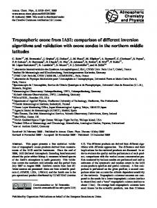
2.2. Block Maxima For the ozone data set, a block length of three days is considered to be a long enough period of separation between observations to achieve independence. In each block, the maxima was obtained (Block maxima). The Block maxima method is described by (Gaines and Denny 1993). The distribution of maximum ozone levels is not the same each year; there is a trend towards lower peak levels of ozone over the years, thus the series is not stationary. Therefore, it is appropriate to analyze and adjust the maximum levels of ozone for each year to minimize the non-stationarity problem. A time series plot for block maxima of ozone levels is in Fig.(1). Autocorrelation in ozone data would have little effect on the bias of parameter estimates, but their variance is affected Vaquera H (1997). The use of block maxima reduces the undesirable consequences of the autocorrelation.

2.3. Parameter estimation for GEV and Dagum In the case of Dagum distribution, the Parameter values for (ˆ a, ˆb, pˆ) that maximize the loglikelihood were obtained using a computational routine in the “VGAM” library for R. The calculation of estimates of the parameters of the GEV model was implemented using the maximum likelihood method with the EVIR package for R. Smith (1985) observed that, for the GEV distribution (11) in the case in which ξ < −1/2, the usual asymptotic distributional properties of maximum likelihood estimators (MLE) do not hold. In contrast, in the case of the Dagum distribution the maximum likelihood estimators do not have such problems according to Kleiber and Kotz (2003). Consequently, if the two models, GEV and Dagum, provide comparable fits to a given data set, an argument can be advanced in favor of using the Dagum model. As we shall see, this is the case for the Ozone data analyzed here.

2.4.

Assessing the of Fit of the Ozone data

The Kolmogorov-Smirnov statistic was used for comparing the Dagum and GEV distribution fits of the ozone maxima time series for each year in the range 2001-2008. The test statistic

Journal of Environmental Statistics

5

0.25

●

● ●● ●● ● ● ● ● ● ●● ● ● ● ●● ● ● ● ● ● ● ● ● ●● ● ● ●● ● ● ● ● ● ●● ● ● ● ● ●● ● ● ● ● ●● ●● ● ● ● ● ●●● ● ● ● ● ●● ● ● ● ● ● ● ● ●● ● ● ● ● ● ● ● ●● ● ● ● ●● ● ● ● ●● ● ● ● ● ●● ● ●● ● ● ● ● ● ● ●● ● ● ● ● ● ● ● ● ● ● ● ● ●● ● ● ● ● ● ● ● ●● ●● ● ● ● ● ●● ●● ● ● ● ●● ●● ● ● ● ● ● ●● ● ●● ● ● ● ●●● ●● ● ●●● ●● ●● ● ● ● ● ● ● ● ● ● ● ● ● ● ● ● ● ● ● ● ● ● ● ● ● ● ● ●●● ● ● ●● ● ● ● ●●● ● ● ●● ●● ● ● ●●● ● ● ● ●● ● ● ●●● ● ● ● ● ● ● ● ● ● ● ● ● ● ● ●● ● ● ● ● ● ● ● ●● ● ● ●●●● ● ●● ● ● ●● ● ● ●● ● ● ●● ● ● ● ● ● ●● ● ● ●● ●● ●● ● ● ● ●● ● ● ● ● ●● ● ●●● ●● ●● ● ● ●●●● ● ● ●● ● ● ●● ● ● ● ● ● ● ● ● ● ● ● ● ● ● ● ● ● ● ● ● ● ● ● ●● ●●● ● ●●● ● ● ●●● ●● ● ● ● ● ●●●● ● ● ● ●●●● ●●● ●● ● ● ● ● ● ●● ● ● ●● ●● ● ● ● ● ●● ● ● ● ● ●● ● ●●● ● ● ● ●● ●●● ● ●● ● ● ●● ●●●●● ● ● ●● ● ● ● ●● ● ● ●● ●● ● ●●● ● ●● ● ● ● ● ● ● ●●● ●● ● ●● ●● ● ● ● ● ● ●● ● ●●● ● ●●●● ●●● ●●● ● ● ● ● ● ● ● ● ●● ● ● ● ● ●● ● ● ● ● ● ●●● ●● ● ● ● ● ● ● ● ●● ● ● ●●● ●● ● ●● ● ● ● ●● ●● ● ● ● ●● ● ●● ● ● ● ●● ● ●● ● ● ● ● ● ● ● ● ●● ● ● ● ● ● ● ● ● ●● ● ● ●● ●● ● ● ● ●●● ● ●● ●● ● ●● ● ● ●● ● ● ●● ●●● ●●● ● ● ● ● ● ● ● ● ●● ● ● ● ●●● ●● ● ● ●● ● ●● ● ● ● ● ● ● ● ●● ● ● ● ● ● ●● ● ●● ●● ● ● ● ● ● ● ● ● ● ● ● ● ● ● ● ● ● ●● ● ● ●● ● ● ●●● ● ● ● ●● ● ● ●● ● ● ● ●● ● ●● ● ●● ●● ● ● ●● ● ●● ● ● ● ●● ●● ●● ● ● ● ● ● ●● ● ● ● ●● ● ●● ● ●● ● ● ● ●● ●● ●● ●● ● ● ● ●● ●●●●● ● ● ● ● ● ● ●● ● ● ● ●● ●● ● ● ● ● ●● ● ● ● ● ● ● ●● ●● ● ●● ● ● ● ● ● ● ●● ● ● ● ● ● ●● ● ● ● ● ● ●● ● ● ● ● ● ● ● ● ● ● ● ● ● ● ● ●● ● ● ● ● ●●● ● ● ● ● ●● ● ● ● ● ● ● ● ● ●● ●●●●● ● ● ●● ●● ● ● ● ● ●● ●● ● ● ● ●● ● ● ● ● ● ● ● ● ● ● ● ● ● ● ● ● ●● ●● ● ● ● ● ●● ● ● ●● ● ● ● ● ● ● ● ● ● ● ● ● ●

0.15 0.05

0.10

Ozone levels

0.20

●

2001

2002

2003

2004

2005

2006

2007

2008

Year

Figure 1: Daily maxima ozone levels for Pedregal (ppm) is: D=

sup −∞