May 6, 2013 - wave-vector kc is simply the Nyquist frequency [3]; one gains nothing by ..... [23] S. E. Koonin, D. J. Dean, and K. Langanke, Phys. Rep.
nt@uw-13-08, int-pub-13-004
Use of the Discrete Variable Representation Basis in Nuclear Physics Aurel Bulgac1 and Michael McNeil Forbes2, 1 1 Institute
for Nuclear Theory, University of Washington, Seattle, Washington 98195–1550 usa of Physics, University of Washington, Seattle, Washington 98195–1560 usa (Dated: May 7, 2013)
2 Department
The discrete variable representation (dvr) basis is nearly optimal for numerically representing wave functions in nuclear physics: Suitable problems enjoy exponential convergence, yet the Hamiltonian remains sparse. We show that one can often use smaller basis sets than with the traditional harmonic oscillator basis, and still benefit from the simple analytic properties of the dvr bases which requires no overlap integrals, simply permit using various Jacobi coordinates, and admit straightforward analyses of the ultraviolet and infrared convergence properties.
arXiv:1301.7354v2 [nucl-th] 6 May 2013
PACS numbers: 21.60.-n, 21.10.-k, 03.65.Ge,
roblems in nuclear physics typically require solving the one-body Schrödinger equation in threedimensions. Numerically representing wavefunctions requires limiting both ultraviolet (uv) and infrared (ir) scales: a finite spatial resolution (i.e., a lattice) characterizes the highest representable momenta Λ, while a finite size (i.e. a cubic box of volume L3 ) determines the largest physical extent. Nuclear structure calculations are historically dominated by the use of the harmonic oscillator (ho) basis of ho wave functions. The appeal of the ho basis stems from the shape of the self-consistent field obtained for small nuclei, which can be approximated by a harmonic potential at small distances from the center of the nucleus. One can also use the Talmi-Moshinsky transformation to separate out the center-of-mass motion in products of single particle ho wavefunctions. Recent efforts have been made to determine a minimal ho basis set, and to understand its convergence and accuracy [1, 2]. Here we advocate that the discrete variable representation (dvr) – in particular the Fourier plane-wave basis – enjoys most of the advantages of the ho basis, but with a significant improvement in terms of computational efficiency and simplicity, thereby admitting straightforward uv and ir convergence analyses and implementation. Consider wavefunctions in a cubic box of volume L3 with momenta less than Λ. The total number of quantum states in such a representation is given by the following intuitive formula – the ratio of the total phase space volume to the phase space volume of a single three-dimensional quantum state:
P
NQS =
�
L 2Λ 2πh
�3
.
(1)
One obtains the same result [3] using Fourier analysis: there are exactly NQS linearly independent functions in a cubic 3d box of volume L3 with periodic boundary conditions and wave-vectors less than kc = Λ/h in each direction. These can be conveniently represented in the coordinate representation with N equally spaced points in each direction and lattice constant a = π/kc = πh/Λ =
L/N for a total of N3 = NQS coefficients. The maximum wave-vector kc is simply the Nyquist frequency [3]; one
gains nothing by sampling the functions on intervals (“times”) finer than a. The wavefunctions can also be represented in momentum space using a discrete fast Fourier transform (fft) [4]. The momentum representation consists of NQS coefficients on a 3d cubic lattice with spacing 2πh/L and extent −Λ 6 px,y,z < Λ. Using the fft to calculate spatial derivatives is not only fast with N log N scaling, but extremely accurate – often faster and more accurate than finite-difference formulas. We use an even number of lattice points (N = 2n is best for the fft) and quantize the three momenta (px,y,z = hkx,y,z ) 2πkh , xk = ak, L � N N k ∈ − 2 , − 2 + 1, . . . , N 2 −1 . pk =
(2)
The Fourier basis uses plane waves – e.g. exp(ikn x) in the x-direction – but these can be linearly combined to form an equivalent sinc-function basis: ψk (x) = sinc kc (x − xk ) =
sin kc (x − xk ) . kc (x − xk )
(3)
This is similar to the difference between Bloch and Wannier wave functions in condensed matter physics. An advantage of this basis is that it is quasi-local ψk (xl ) = δkl allowing one to represent external potentials as a diagonal matrix Vkl ≈ V(xk )δkl [see Eq. (19)]. The plane wave basis can thus be interpreted as a periodic dvr basis set, which has been discussed extensively in the literature (see [5–9] and the references therein), and one can take advantage of Fourier techniques and the useful dvr properties. In general, dvr bases are characterized by two scales: a uv scale Λ = hkc defining the largest momentum representable in the basis, and an ir scale L defining the maximum extent of the system. In many cases, the basis is constructed by projecting Dirac δ functions onto the finite-momentum subspace: For example, the sincfunction basis (3) is precisely the set of projected Dirac
2 δ functions ψn (x) = Pp6Λ δ(~r − ~rα ) onto the subspace |~p| 6 Λ [5–7]. (It can be non-trivial, however, to choose a
consistent set of abscissa maintaining the quasi-locality property.) The basis thus optimally covers the region [−L/2, L/2) × [−Λ, Λ) for each axis in phase space, and leads to an efficient discretization scheme with exponential convergence properties. The dvr basis admits a straightforward analysis of the uv and ir limits, allowing one to construct effective extrapolations to the continuum and thermodynamic limits respectively. The uv effects may be analyzed by simply considering the properties of the projection Pp6Λ used to define the basis, and the ir limit for the periodic basis is well understood by techniques like those derived by Beth, Uhlenbeck, and Lüscher [10, 11]. We would like to emphasize an additional technique here: The ir limit is characterized by 2πh/L – the smallest interval in momentum space resolvable with the basis set. For some problems, one can efficiently circumvent this limitation by using “twisted” boundary conditions ψ(~r + ~L) = exp(iθB )ψ(~r) or Bloch waves as they are known in condensed matter physics. In particular, averaging over θB ∈ [0, 2π) will completely remove any ir limitations (without changing the basis size) for periodic and homogeneous problems, effectively “filling-in” the momentum states pn 6 pn + hθB /L < pn+1 . Extensions of these formulas to the case of a box with unequal sides is straightforward. To demonstrate the properties of the dvr basis, we contrast it with the ho basis. The periodic dvr basis (plane-waves) shares the ease of separating out the center-of-mass. In particular, one can use Jacobi coordinates to separate out the center-of-mass motion without evaluating Talmi-Moshinsky coefficients, leading to simpler and more transparent implementations. The quasi-locality of the dvr basis offers an additional implementation advantage over the ho basis: one need not compute wavefunction overlaps to form the potential energy matrix. In contrast with the ho basis, the kinetic energy matrix K is no-longer diagonal, but it has an explicit formula (23), and is quite sparse, unlike the potential energy operator in the ho basis. Consider the ho wavefunctions with energy E 6 hω(N + 3/2): the maximum radius and momenta are √ R = 2N + 3 b,
√ h Λ = 2N + 3 , b
(4)
p where b = h/mω is the oscillator length. For large N, N ≈ RΛ/2h. Thus, to expand a wavefunction with extent 2R containing momenta |p| < Λ requires at least Nho =
(N + 1)(N + 2)(N + 3) 1 ≈ 6 6
�
RΛ 2h
�3
(5)
states. To contrast, the dvr basis covering the required
volume of phase space (1) with L = 2R and Λ is �
2R 2Λ 2πh
�3
.
(6)
Ndvr 384 = 3 ≈ 12.4. Nho π
(7)
Ndvr =
The ratio in the limit N → ∞ is thus
Since these states are localized, one can further impose Dirichlet boundary conditions, allowing functions only of the type sin(kn x) with kn L = nπ (instead of exp(ikn x)), thereby keeping only half of the momenta: 48 Ndvr = 3 ≈ 1.5. Nho π
(8)
Choosing a cubic box with Dirichlet boundary conditions, sides L = 40 fm, and maximum momentum Λ = 300 MeV/c gives Ndvr =
�
LΛ 2πh
�3
≈ 103 ,
(9)
a somewhat surprisingly small number of states. For symmetric states, one could further the reduce the basis by imposing cubic symmetry, decreasing the basis size by another factor of 8. Finally, one can fully utilize spherical symmetry with a related Bessel-function dvr basis gaining a factor of π/6, and thereby besting the ho basis 8 Ndvr = 2 ≈ 0 .8 < 1 . Nho π
(10)
In this counting, spin and isospin degrees of freedom which occur in both bases have been omitted. The Bessel-function dvr basis set [5–7, 12] follows from a similar procedure of projecting Dirac δ functions for the radial Schrödinger equation. The angular coordinates are treated in the usual manner using spherical harmonics, but the radial wavefunctions are based on the Bessel functions (see Refs. [7, 12] for details) which satisfy the orthogonality conditions Z kc dk 0
2k Jν (krνα )Jβ (krνβ ) = δαβ , 0 (kr k2c |Jν0 (krνα )Jνβ νβ )|
(11)
where zνα = kc rνα [the zeros of the Bessel functions Jν (zνα ) = 0] define the radial abscissa rν,α . The dvr basis set is �z r� √ νn Fνn (r) = rJν , zνn = kc rνn . (12) R Differential operators have simple forms in the dvr basis (see Refs. [5–7] and the codes [13, 14]). In principle, a different basis (and corresponding abscissa) should be used for each angular momentum quantum number ν; In practice, good numerical accuracy is obtained using
3 the ν = 0 basis j0 (z0n r/R) and the ν = 1 basis j1 (z1n r/R) respectively for even and odd partial waves [12, 13]. In the S-wave case, the abscissa are simply the zeros of the spherical Bessel function j0 (z) = sin(z)/z: z0n = nπ,
r0n =
nπ , kc
n = 1 , 2 , 3 , . . . , N,
(13)
and correspond to the 1d basis with Dirichlet boundary conditions mentioned earlier. The zeros for j1 (z) lie between the zeros of j0 (z). The number of dvr functions needed to represent with exponential accuracy a radial wavefunction is N0 dvr =
Rkc , π
(14)
Rkc . 4
(15)
compared to the value 40 A−1/3 MeV one finds in typical monographs [15]. Using only half the value of Λ = 300 MeV/c naturally halves the value of hω. We end with demonstrations of the dvr method [14]. We start with the harmonic oscillator problem in 1d (17)
where we choose the harmonic oscillator frequency according to Eq. (16b), varying the lattice constant a = π/kc and L = Na. The dvr method is sometimes referred to as the Lagrange method in numerical analysis [9], and functions are usually represented on the
hfk |fl i = δkl .
(18)
Potential matrix elements usually have a simple and unexpectedly accurate representation (quasi-locality) Z hfk |V|fl i = dxf∗k (x)V(x)fl (x) ≈ V(xk )δkl , (19) where the functions fk (x) are a linear combination of plane-waves and form an orthonormal set (these formulae apply for even numbers of abscissa as required by efficient implementations of the fft) fk (xl ) =
In the last formula we have divided by an additional factor of 2, since N = 2n + l changes in steps of 2. A major drawback of the ho wavefunctions that is rarely mentioned is that, for modest values of N and l 6= 0, the radial wave functions concentrate in two distinct regions: around the inner and outer turning points of the effective potential V(r) = h2 l(l + 1)/2mr2 + mω2 r2 /2. By adding components with larger values of N, one modifies the wavefunction at both small and large distances, leading to slow convergence. In contrast, the dvr functions are concentrated around a single lattice site. Thus, adding more components only affects the solution in the vicinity of the additional lattice points leaving the states largely unaffected elsewhere. For nuclei one can gain insight with some estimates. Cutoffs of Λ = 600 MeV/c and R = 1.5 · · · 2A1/3 fm should satisfy most of the practical requirements, leading to r hR b= ≈ 0.7 · · · 0.8 A1/6 fm, (16a) Λ h2 hΛ hω = = ≈ 60 · · · 80 A−1/3 MeV, (16b) 2 mR mb
� � k2c x2 h 2 d2 + φ(x) = Eφ(x), Hφ(x) = − 2m dx2 2R2
k
X
N/2−1
to be compared (in the limit N → ∞) with N0 ho =
spatial lattice X ψ(x) = aψ(xk )fk (x),
n=−N/2
�
1 ipn (xl − xk ) exp h L
sin π(k−l) Na
=
cot π(k−l) =0 N
1/a X ψ(xk ) = afk (xl )ψ(xl ),
k 6= l, k = l,
(20) (21)
l
where xk and pn were defined in Eq. (2). As before, the functions fk (xl ) are simply the normalized projections of the periodic Dirac functions on the dvr subspace [5–7], and satisfy X afk (xn )fl (xn ) = δkl . (22) n
The sinc-function basis (3) is obtained in the limit N → ∞ (if a = 1). Similar formulas exist for the calculation of various other spatial derivatives. While the potential matrix is diagonal, the dvr kinetic energy is a matrix in coordinate representation: Kkl =
(−1)k−l h2 π2 mN2 a2 sin2 π(k−l) N� � h2 π2 1 + 2 6ma2 N2
k 6= l k = l.
(23)
This matrix is full matrix in 1d, but sparse in 3d where only 1/N2 of the matrix elements are non-vanishing. The ho Hamiltonian (17) is thus represented in the dvr basis with periodic boundary conditions as Hkl = Kkl +
mω2 a2 k2 δkl . 2
(24)
The implementation of Dirichlet boundary conditions uses the ν = 0 Bessel function basis (see the matlab code [13] for l = 0 and also Ref. [9] for other possible dvr basis sets in 1d). In Fig. 1 we show the energy differences between the eigenvalues of the Hamiltonian (24) and hω(n + 1/2). These “errors” are indicative only of the energy shifts due to the tunneling between neighbouring cells in the case of periodic boundary conditions, as one can judge
101
101
10−1
10−1
10−3
10−3
10−5
10−5
∆E
∆E/hω
4
10−7
10−9
10−11
10−11
10−13
10−13 10−15 0
10
20
30
40
50
n Figure 1. (color online) Difference in spectrum between the dvr Hamiltonian (24) and the ho energies (n + 1/2)hω. The three (blue) curves with pluses have fixed uv scale (lattice constant a = 1, kc = π/a) with L =∈ {30, 40, 50} and ω = 2π/L from left to right. The (red) curves with dots have fixed L = 30 but varying lattice constant a ∈ {1/2, 1/3} demonstrating the uv convergence. The sizes of the dvr basis sets are Lkc /π = 30, 40, and 50 (blue pluses) and 60, and 90 (red circles) respectively. For the blue pluses, the corresponding number of harmonic oscillator wave functions suggested in Refs. [1, 2] (see also Eqs. (4)), would be N = Lkc /4 = Lπ/4a ≈ 24, 31, 39; and 47 and 71 for the red dots, respectively. Notice that the size of the dvr basis set can be reduced by factor of 2 to Lkc /2π = 15, 20, 25 (blue) and 30, 45 (red) respectively, by imposing Dirichlet boundary conditions, however, in that case, states not localized to a single cell will not be reproduced.
by comparing systems with different lengths at the same energy, when the tunneling matrix elements are similar. The results for the lowest 2/3 of the spectrum are, for all practical purposes, converged in the dvr method, and the harmonic oscillator basis set is worse in this case. With N = Lkc /4 ≈ 24 one can obtain at most 10 states or so with a reasonable accuracy in this reduced interval on the x-axis with periodic or Dirichlet boundary conditions, if one were to follow the prescription of Refs. [1, 2]. In Fig. 2 we demonstrate the uv and ir exponential convergence of the dvr method for an asymmetric short-range potential with analytic wavefunctions. Note that both ir and uv errors scale exponentially until � machine precision is achieved – ∆E ∝ exp −2k(L)L (ir) and ∆E ∝ exp(−2kc r0 ) (uv) respectively, where r0 is potential dependent and k(L) is determined by the bound state energy E(L) = −h2 k2 (L)/2m. These exponential scalings follow from simple Fourier analysis (uv) and band structure theory (ir) for short-ranged smooth potentials. Note in particular that the linear uv scaling differs from the quadratic empirical dependence discussed in [1]. We have also demonstrated the utility of the dvr method for a variety of density functional theory (dft) and quantum Monte Carlo (qmc) many-body calculations.
UV
10−7
10−9
10−15
IR
0 5 10 15 20 25 30
L
0
5
10
15
20
kc
Figure 2. (color online) Exponential convergence of the periodic dvr basis for the energy of the bound states of the analytically solvable Scarf II potential V(x) = [a + b sinh x]/ cosh2 x (with h = m = 1). For a = 7/2 and b = −11/2, the potential has three bound states – En = −(3 − n)2 /2 (shown in black, blue, and green from left to right respectively). The left plot demonstrates the ir convergence for increasing L with fixed kc ; the right plot demonstrates the uv convergences for increasing kc for fixed L. The various values for kc ∈ {5, 10, 15, 20} (left) and L ∈ {5, 15, 25, 35} (right) correspond to dotted, dotdashed, dashed, and solid lines with increasing convergence respectively.
The Bessel-function dvr basis jl (Λrn /h) for spherical coordinates was used in [13, 16] to solve the selfconsistent superfluid local density approximation (slda) dft equations for the harmonically trapped unitary Fermi gas. While the basis is defined for all l, even and odd l-partial radial wave functions can be effectively expressed using only the j0 and j1 basis sets respectively (see [12]) with the angular coordinates represented by spherical harmonics. The spatial mesh size is given by ∆r = rn+1 − rn ≈ πh/Λ. Applied to nuclear matter, Λ = 600 MeV/c gives ∆r ≈ 1 fm and Ns = R/∆r ≈ 20 radial mesh points in a spherical box of radius R ≈ 20 fm. A matlab code for a spin imbalanced trapped unitary gas with pairing and using two different chemical potentials for the spin-up and spin-down fermions respectively, is about 400 lines and converges in a few seconds on a laptop [13, 14]. The periodic dvr basis was used in Ref. [17] to solve the self-consistent slda dft, predicting a supersolid Larkin-Ovchinnikov (lo) phase in the spin imbalanced unitary Fermi gas. Explicit summation over Bloch momenta was used to remove any ir errors (i.e. simulating a periodic state in infinite space rather than in a periodic space.) The periodic basis was also used in [18] to demonstrate the Higgs mode by solving the timedependent slda for systems with up to 105 particles. (In both these approaches, spatial variations were only allowed in one direction: transverse directions were treated analytically.) Full 3d periodic dvr bases were used in [19] to solve
5 0 −10
“triton” 1VPT “triton” 2V2G “α” 1VPT
E (MeV)
−20 −30
“triton” 4V2G
−40 300 200 100 −60 0 −100 −70 −200 0 −50
0.00
4V2G “α” 1.5VPT
4VPT
3
6 0.10
0.05
0.15
L−1 (fm−1 ) Figure 3. (color online) Binding energy of a three-particle “triton” and four-particle “alpha“ ground state using various multiples (specified by numerical factors in the figure) of the potentials VPT (r) ∝ −sech2 (2r/r0 ) and V2G (r) ∝ exp(−r2 /r20 ) − 4 exp(−4r2 /r20 ) with r0 = 3 fm (see [24] for explicit normalizations). Upper and lower bounds are obtained from Dirichlet and periodic boundary conditions respectively. The deeply bound four-body state with 1.5VPT is not converged and has comparable uv and ir errors (each “band” has fixed lattice spacing). The other results are uv converged: the different lattice spacings lying on the same curves describing the dependence on the box size. The inset shows the radial profile of the two potentials.
the time-dependent slda equations for 48 × 48 × 48 and 196 × 32 × 32 lattices, solving ≈ 5 × 10⁵ non-linearly coupled partial-differential equations for several million time steps to study the real-time dynamics of the superfluid unitary Fermi gas. Extensions of this code on current supercomputers allow us to increase the overall size of such problems by an order of magnitude. These 3d dvr bases were also used to study the giant dipole resonance (gdr) in deformed triaxial open-shell heavy nuclei [20] without any symmetry restrictions. Finally, the 3d dvr basis was used in [21] (and earlier references therein) to perform ab initio qmc calculations of strongly interacting fermions in spatial lattices ranging from 63 = 216 to 163 = 4096 for systems comprising 20 to 160 particles and with 5000 steps in imaginary time. These systems are significantly larger than the 364 single-particle states used in [22] to implement a nuclear shell-model qmc [23]. Similar applications of dvr qmc are currently being developed for nuclear systems. We further illustrate the power of the dvr basis in Fig. 3 by solving the 6d and 9d Schrödinger equations for three-body (“triton”) and four-body (“α”) bound states with distinguishable particles interacting with two centrally symmetric potentials: a purely attractive
Posh-Teller potential, and an attractive potential with a repulsive core (see the inset). We used a Cartesian lattice for the relative Jacobi coordinates to eliminate the centerof-mass coordinate. Our goal was to solve these with a modern laptop (2.7 GHz Intel Core i7 MacBook Pro with 16 GB of ram) in no more than about a few minutes, without any tricky optimizations such as taking advantage of symmetry properties of the wavefunction. (Parity alone could reduce the Hilbert space by factors of 26 and 29 respectively.) Coding these problems is simple – the matlab versions are about 200 lines per problem while the general Python code is about 1000 lines (including documentation and tests) [14]. We are not aware of other attempts to solve directly the Schrödinger equation in a 9d-space. To compute the ground state energy, we use two alternative techniques: imaginary time evolution of a trial state (slow convergence but gives a representative wavefunction) and a simple Lanczos algorithm (fast convergence, but only a few low-energy eigenvalues). For the triton we used lattices N6s = 86 · · · 166 : for the α state we use lattices N9s = 49 · · · 89 . The size of the largest Hilbert space is thus ≈ 1.68 × 10⁷ for the triton and 89 ≈ 1.34 × 10⁸ for the α. Several spatial mesh sizes a =0.5 fm · · · 1.5 fm corresponding to Λ ≈ 300 MeV · · · 930 MeV/c are used to explore convergence. Note that, unlike with other methods used for nuclear structure calculations, adding local three-body and fourbody interaction will neither complicate the code nor impact the performance. As discussed earlier, the uv convergence is determined by the properties of the interaction: For example, the high-momentum components of a wavefunction in a short-range potential will have a power-law decay ∝ k−4 [25] (rather than an exponential decay). The ir convergence of the energy will be determined by the energy of the lowest many-body threshold. For example, if there is an S-wave two-body threshold with binding energy difference Q(L) in the box, then the ir error will be [11] p A exp(− 2MQ(L)L/h) E(L) ≈ E∞ + (25) L where M is the corresponding reduced mass, and A an asymptotic normalization factor that is positive or negative for Dirichlet or periodic boundary conditions respectively. If the lowest threshold is higher-body or in a different (not S-wave) configuration, then this behaviour will be modified in a straightforward manner. (Competition between several closely lying thresholds will further complicate the ir convergence properties.) Note that this differs from the results of [1, 2]. In summary, the dvr basis seems ideal for nuclear structure calculations using either dft, qmc or configuration mixing approaches. It is near optimal in size, and can deliver results with exponential convergence. The dvr basis shares the important advantages of the
6
ho basis set: efficiently separating out the center-ofmass motion using Jacobi coordinates (with the added benefit of not needing to evaluate Talmi-Moshinsky coefficients), utilizing symmetries to reduce the basis size (spherical with the Bessel function dvr). Moreover, matrix elements are easy to evaluate – the potential matrix is diagonal for local potentials (no overlap integrals are needed – see for example Eq. (19)), the kinetic energy matrix is sparse and explicitly expressed analytically, and many-body forces can be easily included. Further-
more, the uv and ir convergence properties of the basis appear on a equal footing, and are clearly expressed in terms of the momentum-space projection and finite box size, allowing for simplified and sound convergence analysis, with a clear mathematical underpinning. Finally, we demonstrated that the dvr basis can be used in extremely large Hilbert spaces with relatively modest computational resources. We thank G.F. Bertsch for discussions and the support under us doe grants de-fg02-97er41014, de-fc02-07er41457, and de-fg02-00er41132.
[1] R. J. Furnstahl, G. Hagen, and T. Papenbrock, Phys. Rev. C 86, 031301 (2012), arXiv:1207.6100. [2] S. A. Coon, M. I. Avetian, M. K. G. Kruse, U. van Kolck, P. Maris, and J. P. Vary, Phys. Rev. C 86, 054002 (2012), arXiv:1205.3230. [3] R. W. Hamming, Numerical Methods for Scientists and Engineers (McGraw-Hill, Inc., New York, NY, USA, 1973). [4] The Fastest Fourier Transform in the West, www.fftw.org, developed by M. Frigo and S.G. Johnson. [5] R. G. Littlejohn and M. Cargo, J. Chem. Phys. 116, 7350 (2002). [6] R. G. Littlejohn, M. Cargo, T. Carrington, Jr., K. A. Mitchell, and B. Poirier, J. Chem. Phys. 116, 8691 (2002). [7] R. G. Littlejohn and M. Cargo, J. Chem. Phys. 117, 27 (2002). [8] D. Baye, J. Phys. B 28, 4399 (1995). [9] D. Baye, physica status solidi (b) 243, 1095 (2006). [10] E. Beth and G. E. Uhlenbeck, Physica 4, 915 (1937). [11] M. Lüscher, Comm. Math. Phys. 104, 177 (1986); S. R. Beane, P. F. Bedaque, A. Parreño, and M. J. Savage, Phys. Lett. B 585, 106 (2004), arXiv:hep-lat/0312004. [12] N. Nygaard, G. M. Bruun, B. I. Schneider, C. W. Clark, and D. L. Feder, Phys. Rev. A 69, 053622 (2004), arXiv:cond-mat/0312258. [13] http://www.phys.washington.edu/%7Ebulgac/ numerical_programs.html.
[14] https://bitbucket.org/mforbes/paper_dvrvsho. [15] A. Bohr and B. R. Mottelson, Nuclear Structure (World Scientific, Singapore, 1998). [16] A. Bulgac, Phys. Rev. A 76, 040502 (2007), arXiv:condmat/0703526. [17] A. Bulgac and M. M. Forbes, Phys. Rev. Lett. 101, 215301 (2008), arXiv:0804.3364 [cond-mat]. [18] A. Bulgac and S. Yoon, Phys. Rev. Lett. 102, 085302 (2009). [19] A. Bulgac, Y.-L. Luo, and K. J. Roche, Phys. Rev. Lett. 108, 150401 (2012), arXiv:1108.1779. [20] I. Stetcu, A. Bulgac, P. Magierski, and K. J. Roche, Phys. Rev. C 84, 051309(R) (2011), arXiv:1108.3064 [nucl-th]. [21] G. Wlazłowski, Gabriel, P. Magierski, J. E. Drut, A. Bulgac, and K. J. Roche, Phys. Rev. Lett. 110, 090401 (2013), arXiv:1212.1503; J. E. Drut, T. A. Lähde, G. Wlazłowski, and P. Magierski, Phys. Rev. A 85, 051601 (2012), arXiv:1111.5079 [nucl-th]. [22] C. N. Gilbreth and Y. Alhassid, (2013), 1210.4131:arXiv [cond-mat.quant-gas]. [23] S. E. Koonin, D. J. Dean, and K. Langanke, Phys. Rep. 278, 1 (1997). [24] M. M. Forbes, S. Gandolfi, and A. Gezerlis, Phys. Rev. A 86, 053603 (2012), arXiv:1205.4815. [25] R. Sartor and C. Mahaux, Phys. Rev. C 21, 1546 (1980); S. Tan, Ann. Phys. (NY) 323, 2971 (2008), arXiv:condmat/0508320.