model parameters simultaneously by using P-wave arrivals from local earth- quakes at a local seismograph ..... first one is Franklin's (1970) stochastic inverse. ...... A Backus-Gilbert approach to inversion of travel time data for three diinensional ...
Geophys. J. R. astr. SOC.(1983) 75,431-412
Use of two inverse techniques. Application to a local structure in the New Hebrides island arc
J. R. Grasso Institut de Recherches Interdisciplinaires de Ge'ologie e t de Me'canique, Laboratoire de Giophysique Interne, Universite' Scientifique et Midicale de Grenoble, BP 53, 38041 Grenoble Cedex, Francr
no. 154, RCP FroblPrnes Inverses no. 264, Universite'des Sciences et Techniques du Languedoc, 34060 Montpellier Cedex, Francr
G. Pascal
Laboratoire de Giophysique Marine, GIs no. I 2 'Ocianologie et Giodynamique ' CNRS-CNb'XO-UBO, Universite' de Bretagne Occidentale, 6 , Avenue Le Gorgeu 29283 Brest Cedex, France
Received 1983 March 21 ; i n original form 1982 February 3
Summary. Two inversion techniques (stochastic inverse and linear programming) are used in the determination of hypocentre and velocity model parameters simultaneously by using P-wave arrivals from local earthquakes at a local seismograph array. These procedures are applied to P-wave data obtained from a combined land and ocean bottom seismographs network in the New Hebrides island arc. Two hundred and fifty-two residuals data are inverted simultaneously with 46 earthquake parameters. The displacements of each initial hypocentre location are practically the same with the two methods and are small (2--4km). The main result for the velocity model parameters is the existence at a low-velocity zone between depths of 10 and 1 9 k m and may be deeper. An estimate of the degree of confidence of the solution is determined and can confirm that the extremal values of the 7.3 km s-' are 7.2 and 7.5 km s-'. These results may be related to an intrusion of ultrabasic magma from the mantle beneath Malekula and Efate Islands. 1 Introduction With thc increasing prevalence of large seismograph arrays and the development of a method for the seismic imagery of the Earth ( M i , Christofferson & Husebye 1977), a new opportunity is provided to study the structure of a part of an island arc in detail. Although many papers have been published on the seismicity of the New Hebrides island arc (Dubois 1969; Santo 1970; Isacks & Molnar 1971; Barazangi et al. 1973; Pascal et al. 1973, 1978; Chung & Kanamori 1979; Cardwell et al. 1979; Isacks et at. 1981; Coudert ef al. 198l), very few
Downloaded from http://gji.oxfordjournals.org/ by guest on November 4, 2015
M . Cuer Laboratoire de Physique Mathimatique e t The'oorique, E R A CNRS
438
J. R. Grasso, M. Cuev and G. Pascal
2 Data selection 2.1
RESIDUALS
For a period of four weeks in 1978 September, a combined land and ocean bottom seismographs network covered the central part of the New Hebrides island arc and was operated by ORSTOM, Cornell and Texas Universities. This survey, like the previous one (Coudert et 01. 1981 for example), was included in a cooperative project carried by the three groups for
Downloaded from http://gji.oxfordjournals.org/ by guest on November 4, 2015
investigations have been devoted to the study of the crustal and upper mantle structures (Dubois ef al. 1973; Louat, Dubois & Isacks 1979; Goula & Pascal 1979). Before attempting to model real data and to interpret the crust and upper mantle anomaly patterns, we will have t o discuss some aspects of the problems and the difficulties which arose in this study. In the inversion method, the travel-time residuals of P-waves from local earthquakes and a geometrical discretization are used in generating the test data. The discretization consists in using a stack of homogeneous layers with horizontal boundaries. We choose t o explain the travel-time residuals in terms of relative variations of the isotropic velocity and perturbations of the geographical and temporal parameters of the earthquakes. The two sets (data and unknown parameters) are expected to satisfy a linear approximation. At this stage we notice that it is adequate to use classical statistical methods (least squares) for an estimate of the unknown parameters, when the dimension of the unknown vector is small compared to that of the data vector. In the previous studies using the inversion method developed by Aki et al. (1977), Crosson (1976), Chou & Booker (1979), Spencer & Gubbins (1980), Pavlis & Booker (1980), Gubbins (1981) and Jordan & Sverdrup (1981), and applied by Ellsworth & Koyanagi (1977), Mitchell, Chang & Stauder (1977), Zandt (1978) and Goula & Pascal (1979), an over-determined system of linear equations is then solved by least squares inversion. In our case the statistical formulation used in these papers raises some fundamental problems: according to the choice of the number of discrete parameters, we have t o solve, with the same set of arrival times, either an over- or under-determined system. Then we have to solve a system with a unique solution, which never fits exactly the data, or a system which gives several solutions. Such remarks would weaken the inversion process. They only convince us that it is necessary to develop a new interpretation of the three-dimensional inversion method. The choice of the discretization can mask the inherent non-uniqueness of the solution in these problems and should be guided by physical criteria. The importance of this choice is discussed in Section 2. It has to be considered here as a part of the assumptions which are used to build the solution. To solve this ambiguity we prefer to admit that some new physical constraints are necessary to interpret the data. So we present in Section 3 the formulations of the two techniques which are useful to cross the over-/under-determined system barrier; the linear programming technique which allows us to use explicit bounds to compute several solutions and to particularize them, and, the stochastic inverse method where the a priori knowledge is formulated using probability laws. Then by means of these two procedures the data are fitted in the damped least square sense (L2 norm) and constrained L 1 norm (Section 4). We have also used the constrained L , norm on a restricted set of our data. We show that the solutions computed by the two methods can be correlated and present an unexpected consistency in their variations, as well for the earthquake parameters as for the velocity structure. Then an attempt to measure the degree of confidence of the results is presented (Section 5 ) . Finally the crustal and upper mantle anomalies are interpreted in a geodynamical context.
Use o j t w o inverse techniques 167OE
439
169O
15'
15O
190
190
167OE
169O
Figure 1. Map view of the central New Hebrides area showing the topography (in fathorns) and the islands o f the studied area. Solid triangles indicate ORSTOM multicomponent seismograph stations, solid circles the stations oT the permanent network and solid squares the Ocean Bottom Seismographs (OBS).
Downloaded from http://gji.oxfordjournals.org/ by guest on November 4, 2015
1705
17O!
440
J. R. Grasso, M. Cuer and G. Pascal
--__ I X
2
I I-
2i Figure 2. Velocity model derived from the refraction experiment. The dashed line is obtained only from the southern profile; then this root is drawn here only as an indication. On the right side we present the homogeneous layers with parallel interfaces we used as an initial model for the inversion process.
many years. The ocean bottom seismographs were built by the University of Texas; the land stations, operated by the three groups, are stations of the permanent network in the New Hebrides arc (ORSTOM and Cornell) and temporary stations from Cornell University. All the collected seismograms were read by ORSTOM in Noumea and preliminary earthquake locations were determied using the H Y P O 7 1 computer program (Lee & Lahr 1975). At our request, ORSTOM kindly provided the readings of about 100 events. The array consisted of 17 stations in an area between 16"s and 18"sand 167"E and 169"E (Fig. 1). To invert the data set, we must first set up an initial model and calculate the arrival times. As an initial model for the structure under the array, we used a crustal structure very close to that derived from a seismic refraction experiment (Ibrahim et al. 1980). This experiment took place in the south of the area, between 18"sand 20"s (Fig. 2). The next step of the data analysis is the generation of the set of rii residuals:
For each event i, we compute the rii (station indexj) by a classical least squares determination of hypocentre parameters. These rii are greater than the reading errors. We have selected 46 events for this study (Table 1). FoJr criteria were used for the selection of the events (see also Section 2.2): (1) 10 arrivals ( P and S) at least for each location; (2) events on the margin or outside of the network were rejected; (3) only events with stable focal parameters for different initial depth were selected; (4) residuals greater than 0.7 s were rejected. Fig. 3 is a location map of the array showing the sites of the 17 stations used in this study and the event locations of the final set of 46 earthquakes. The S-waves, being of lower quality, have not been used in the inversion. Initially we decided to study separately the Efate island region and the Malekula island region because of the uneven earthquake 'istribution. Different tests showed us that more information could be provided with the two seismic regions together. So except for Figs 5 and 6 the numerical results are based on the second choice. We point out here that the study of the individual regions gives a slightly
Downloaded from http://gji.oxfordjournals.org/ by guest on November 4, 2015
R
Use of two inverse techniques
44 1
Table 1. Comparison of initial hypocentres and revised hypocentres. N" 1
2 3 4
5 6
7 8 9
10 11 12 13
x
111.47 -58.28 -48.49 -49.18 -51.62 -49.23 -48.07 -45.25 -62.67 -52.50 -43.18 -62.98 -44.41
14 15
-38.45
16
-60.29
17 18
19
20 71
27 23 2r> 26 27 28 29 30
31 32
33 14
35 36 37 38 34 '
a0 41 42 43 44
45 46
-23.48 -98.08 -92.40 -50.35 -131.no -80.78 -55.43 -90.73 -26.59 107.51 -57.66 -54.07 -40.07 34.97 88.43 90.27 49.85 43.81 170.05 12.69 28.51 68.16 74.47 121.38 78.96 4R.93 44.59 72.73 22.21
2
AX1
54.89 12.39 29.36 15.02 16.68 21.04 21.71 28.27 27.93 20.59 33.11 29.b5 42.67 43.44 39.53
-5.000 -1.390 -5.000 -0.245 -1.220 1.390 5.000 U ,030 1.580 -0.050
48.56
3.040
-21.46
-43.96 -61.96 -35.84 -21.27 -30.40 -1.77 -6.05 -5.67 -22.77 -26.68 -6.33 -17.03 -2.56 -33.20 -36.63 -7.03 -26.29 -12.49 -24.09 -6.84 -35.94 -3.3s 136.84
45.96 42.57 35.23 60.58 33.24 43.68 45.32 66.79 34.72 56.46 29.49 38.97 31.19 25.75 34.67 13.30 15.10 25.51 34.14 20.61 15.62 39.29 16.50 37.50 14.56 13.02 36.80 31.26 29.47 49.75
-5.000 -3.120 5.000 -0.064 -5.000
-5.000
AY1 3.430 -1.810 -4.500 -1.810 -0.265 -0.496 -3.050 -0.931 0.345 -2330 2.780 -2.070 1.110 0.975 1.310 -0.932 2.650
-4.710 4.550 -0.427 1. 480 0.317 -5.000 -5.000 -0.921
-
-3.480
-5.000 -1.010 -1.070 3.690 -5.000 -0.147
1.650 -0.186 2.800 0.915 0.407 4.080 -5.000 3.760 -2.000 3.R30 -5.000 4.520
0.284 0.379 5.000 1.890 5.000 0.504
A21
-0.784 5.000
-5.000 5.000 -1.040
-1.530 -3.040 -1 ,190 5.000 5.000 3.320 4.690 -0.261 4.000 -0, 500 3.610 -0.220 5 . oon 0.396 5.000 -0.332 2.330 0.500 5.000 -0.088 5 . no0
500 5 . no0 -0.500 -5.000
5.000 -1.360 5.000 -0.253 -3.700 2.690 -0.402 -3.660 -5.000 0.957 -3.910 0.643 -5.000 -5.000 -5.000 3.990 -1.960 5.000 1.910 2.370 -1.480 1.970 0.084 1.470 0.425 2.920 -3.210 5.000 5.000 -4.900 -5.000 -1.260 0.330 -0.413 -5.000 1.200 - U . 750 -0.393 -5.000 1.220 5,000 2.330 -2,800 -1.610 -5.000 4,670 5,000 2.970 -5.000 -0.b94
A t1 0,206 -0.213 0.465 -0.304 0.159 0.042 -0.271 -0.250 -0.181 -0.000 0.500
-0.
-0.225 -0.192 -0.35s 0.500 0.063 0.500 0.500 0.479
-0.156 -0.105 -0.500 -0,274
AX2
AY2
-2.102 0.875 -0.549 -0,629 -3.151 -3,474 0.a99 -1.294 0.138 1.622 0.462 0.136 3.561 -2.455 1.631 -11.996 0.932 1.033 -1.253 -1.3'10 -0.486 0.537 -1.858 -2.176 3.289 1.124 -1.426 0.023 -4.356 -1.052 1.924 - I r 122 -0.722 -1.158 -2.971 3.321 l.2dl -0.559 0.477 -4.R16 -1.168 -1.780 -1 .449 -1.707 -1.861 -2.155 0.494 -3.0'/9 -1.200 -0.582 0.706 -1.970 -1.719 -1.625 1 . 4 9 1 -1.379 -1.148 -3.496 -2.633 3.550 0.044 2.'131 0.4R0 1:744 -0.04? 1.469 2.577 -0.016 -1.716 0.966 0.30G 2 . 248 -0.500 -0.305 1.074 -0.233 0.721 0.4R8
0.093 -0.167 0.057 -n.n31 -0.500 -0.321 -0.500 2.0n5 -0. 500 0.297 -0.398 -0.098 -C.368 1.895 0.1'78 0.000 0.417 -0.172 3.032 -0.389 0.348
A22
3.551 10.707 -1.962 1.916 -0.725 1.121 -2.383 -1,170 2.022 3.919 1.380 -0.916 -1.29R -0.419
At2 0.036 -0.1c12 0.093 -0.079 0.007 0.014 -0.200 -0.006
0.013 0.024 0.027 -0.013 -0.095 -0,001
4.106 0.028 0.717 -0.013
n .n58
n .n27
3.539 n .o x 1.279 -0.008 -1.952 -0.078 -1.182 c on9 cl.822 0.003 1.159 -0.014 -0.190 0.01? 1.?If, o.mu 1.410 0.028 -C.03/ 0.07C -3.239 0.037 -?.490 -0.007 -1.035 -0.015 0.36G -0.041 -0.79n -0.004 0.904 0.032 -0.464 -0.04F 0.373 o.nic -0.053 -0.10P 0.224 0.005 -0,677 0.001 -0.227 -0.005 -1 ,906 0.00' -1 .UfiR -0.712 -0.138 -0.001 4.281 -0.065 0.731 0 . 2 8 8 -0.142 0.010 -1.4a2 -1.731 0.017 2.083 0.633 0.012 -0.947 -0.088 0.002
.
over-determined system whereas the study of the total area gives an under-determined system for the same block size. The difference is explained by the fact that, when the two regions are grouped, the increase of the number of data (observations of northern events at the southern stations and reversely) is smaller than the increase of the number of unknowns.
2.2
GEOMETRICAL DISCRETIZATION A N D FINAL SELECTION O F RESIDUALS
The simplest way to build the 3-D seismic 'image' of the area is to use discrete models. Such a procedure requires the choice of the block size for the discretization. There is no exact mathematical process to justify this choice since the data are a finite number of 'curve integrals'
and the unknown AV/Vo(r) is a function of three variables. However, one can hope that such a justification could be made in relation to the wavelength (less than 10 km in most of the previous studies and about 1 km for local earthquakes) if the theory of wave propagation should allow us to write the perturbation to the arrival times ds
AV
Downloaded from http://gji.oxfordjournals.org/ by guest on November 4, 2015
24
-42.13
Y -14.72 -10.10 -27.09 -18.33 -22.04 -27.95 -24.29 -29.32 -21.78 -26.26 -50.48 -36.14 -21.85 -23.01 -25.22 -41.01 -40.52 -14.27 -7s.55 -7.00 -41.03 -18.54 -8.91
44 2
J. R . Grasso, M. Cuer and G. Pascal
,
0
\
v
\
.
O
V
\
\ \
0
\
\
\
0
0
V
v 0 0
.
\ I
-
\
iN v ,
\, b-
r-'\
\ \
\
v v
\% \
0
. ./ -
L/-
\,
. 0 20km
\
i
I---
I -
/-
//-
I
Figure 3. Locations of the events used i n this application. They all occurred in the period 1979 September 14-30.
as a 3-D mean
the lateral extent of the 'integration tubes' tube, being of the order of t h e wavelength. In fact only a geophysical o r geological a priori provides a good criterion.
Downloaded from http://gji.oxfordjournals.org/ by guest on November 4, 2015
\
\,
-
Use of two inversp techniques
443
In looking for a good compromise between a relatively large number of unknowns (and then some freedom for the solution) and the number of rays inside each block, the geometrical discretization is built as follows: (1) In the shallowest layer we choose a station-block model: the results in these blocks may correspond to station-term anomalies (see, e.g. Crosson 1976) and could take into account the possible bias due to the instrumentation. (2) The other layers are chosen to fit the initial crustal structure except the fourth one which is divided into two sublayers of relatively small blocks in order to obtain ‘acceptable results’ with the stochastic inverse.
Fig. 4 shows the chosen discretization: the number of rays inside each of the 216 blocks is given in Fig. 7. Note that different applications of this modelling process with the stochastic inverse show stable solutions (for teleseismic data) when the blocks are moved horizontally (see Ellsworth & Koyanagi 1977; Goula & Pascal 1979 for example). Besides one observes here stable velocity anomalies when the block sizes are chosen slightly smaller (with the stochastic inverse). But these experimental tests are not sufficient to remove the theoretical ambiguity. We want to underline that the apparent arbitrariness of the discretization is not a good argument for rejecting the technique. A realistic example of such a situation is the tomography. In this example, the solution with a finite number of data is non-unique but the quality and the distribution of the data offer a good guarantee for the results except in few cases, although here also there is no rigorous justification of the discretization process. Note finally that some rays are refracted and lead to the following problem. Even when the discontinuities introduced by the choice of the layer interfaces are well recognized, a large number of refracted seismic rays can perturb the solution in the blocks just below or above the discontinuity, especially when few other rays cross such blocks. Since one can
Downloaded from http://gji.oxfordjournals.org/ by guest on November 4, 2015
Figure 4. The geometrical discretization. Solid triangles are the station sites.
J. R . Grasso, M. Cuer and G. Pascal
444
consider that such rays propagate either below or above the discontinuity we have chosen to work only with upgoing rays so that the total number of data used is 252 arrivals of P-waves. 2.3
A PRIORI BOUNDS O N THE PARAMETERS A N D ABSTRACT O F THE INPUT IN F O R M A T I O N
‘Statistical bounds’ GAV/V, UAX
Explicit bounds
=0.15
= G A Y = UAZ = 4.76 km
oAT=o.15
-0.15
G
AV/Vo < 0.15
-5 km
G
A X , AY, AZ
-0.5 s
G
AT
G
Q
5 km
0.5 s
The reading error on arrival times has been estimated to be 0.1 5 s so that the so-called 6’ parameters of the stochastic inverse are 0.15
OAVJV0-
--
~
aAV/V,,
=I,
0.15 BAT=-GAT
-1,
0.15 8Ax=-
=0.03=B*y=BAz. @AX
Ln summary the input information is the following. We have used an initial velocity model derived from a seismic refraction experiment which gives a preliminary determination of hypocentre parameters for the 46 chosen earthquakes recorded at 17 stations. We have then selected 252 arrivals of P-waves and finally we have chosen a discretization in 21 6 blocks and some bounds on the 400 unknowns. 3 Mathematical formulation of the inverse techniques 3.1
L I N E A R I Z A T I O N OF THE PROBLEM BY YERMAT’S P R I N C I P L E
Each observation is associated with a ray, say rayk which ends at t h e j k t h station and comes from the i,th hypocentre; the hypocentre parameters are t i k (origin time) and x i k , y i k ,zik (coordinates). Using Fermat’s principle one can compute the variation of the arrival time along this ray
corresponding to a first-order variation At,,, A x i k , A y i k , A z i k , AV(r) of the model parameters:
Downloaded from http://gji.oxfordjournals.org/ by guest on November 4, 2015
Our previous heuristic choices give a system with 252 data (252 P-wave arrivals from 46 earthquakes at 17 stations) and 400 unknowns (216 relative velocity variations in 216 blocks and 4 x 46 = 184 earthquake parameters). Clearly this system is under-determined and some constraints on the unknowns are necessary. These constraints are expressed in a statistical way for the stochastic inverse technique and are explicitly written when we use the linear programming techniques. Guided by the geophysical literature on the studied region we have adopted the following bounds, where AV/Vo refers to the relative velocity variations of P-waves, and AX, AY, AZ,AT to the variations of hypocentre parameters:
Use o f two inverse techniques
445
Introducing as unknowns the vector m = (mH, m"), where
mH =(Ati,Axi,Ayi,Azi,
. . . ,At46,Ax46,AY46,AZ46jT
and
mv =
, . ' .>
F)
T
,,,)
is the relative variation of the velocity inside the 216 blocks; the residuals de = Tik, ik must satisfy the linear system: 4 X 46
dk
=
(Gm), =
1 g21
+
216
1
g z l m y for k = 1, 2, . . . , 2 5 2
I =I
1=1
3.2
T H E TWO T E C H N I Q U E S USED T O FIT T H E DATA
In order to compute solutions of the linear system (1) we have used two techniques. The first one is Franklin's (1970) stochastic inverse. In this technique the a priori statistical bounds of Section 2.3 are written in terms of the apriori covariance matrix:
C,
= diag(uh)
for the model parameters (urn = 0.1 5 for the relative velocity variations and the origin times of earthquakes and u, = 4.76 for the hypocentre locations) and: Cd =
diag(u:)
with ad = 0.15 s for the errors on the residuals d k . The estimation of m of mifiimal variance is then: m = C, GT(GCrnGT f Cd)-'d or in an equivalent way:
which is obtained by minimizing (Gm - d)T Cjl(Gm - d) the diagonal elements of Cd are equal,
k=l
I= 1
f mTCilm
that is to say, since all
Downloaded from http://gji.oxfordjournals.org/ by guest on November 4, 2015
is the travel time of the kth ray inside the Ith block.
J. R. Grasso, M.Cuer and G. Pascal
446
with 0; = 1 for the velocity and origin time parameters and 0: = m 3 ' 4 0.001 for the hypocentre location parameters. The covariance of m - m is given by (Franklin 1970):
c,
(3 1
-C,GT(GC,GT+CJ'GC,
so that the lth diagonal element of the matrix C, GT(GC, GT + C d ) - ' G is the relative variance improvement or the so-called resolution Rl of the parameter mI. For the inversion of the matrix GC, GT + Cd we have used the Cholesky method. The second technique is the linear programming (see Dantzig 1963), the use of which in geophysics has been proposed by Sabatier (1977) and Huestis & Parker (1977). This technique allows us to compute bounds on some linear function of a vector, this vector being subject to linear equalities or inequalities. Here one can think for example to compute bounds on the average of the relative velocity variation in some area, that is to say:
c
I index 1 such that
):A(
I
x volume of blocki
(4)
the block! belongs to the given area
m (and in particular (AV/Y),)being subject to dk
-
0.15
- n y x
-
(G m)k < dk + 0.15
< mI
Q
m y x
. . . , 252 1 = 1 , 2 , , . . ,400
k = 1, 2,
(5)
(where the bounds m y a x = 0.15 for the relative velocity variations, mTaX= 5 km for the hypocentre location parameters and myax = 0.5 for the origin times of the earthquakes). Using linear programming it is also possible to compute the smallest relative velocity variation in a given area that is to say: min
SUP
index 1 such that the block1 belongs to the given area
l(~V/Vo)rl)
the parameters being subject to (5). But here the inequalities system (5) has no solution, and we have used the linear programming techniques to minimize the misfit Gm - d . Two kinds of misfits have been used. The first is the L , misfit that is SUP k - I , . . ., 2 5 2
I (Gm-d)k I.
The linear programming problem to solve is then, optimization jargon:
(Y
being called a 'slack' variable in the
min a when a and m satisfy: -a
Q
(Gm-d)k Q , m , ~mmax
- mrnax
t
k = 1, . . . , 2 5 2
I
= 1 , . . . , 400.
(7)
The result gives the smallest reading error compatible with the data dk and the a priori bounds myax.
Downloaded from http://gji.oxfordjournals.org/ by guest on November 4, 2015
min and max of
Use of two inverse techniques
447
The second is the L misfit 252
I(Gm-d)kI, k=l
the corresponding linear programming problem being, with ak k = 1 , . . . , 252 as 'slack' variables: 252
min
1
o(k
k=l
where "k and m satisfy
must satisfy the optimum (necessary condition for a minimum):
So we have attempted to compare the resolution R, obtained with the stochastic inverse with the number Ul (see Section 4) but this is only an attempt and in our opinion the only way to define a resolution in the context of explicit a prbri bounds is the computation of a posferiori bounds as those of the average relative velocity variation in a given area (see Section 5 ) . For the linear programming computation we have used the F O R T R A N routines of Cuer & Bayer (1980). We do not claim to have made a conceptual comparison between the two approaches (statistical and explicit bounds) but we think we have made a comparison of what can be done with the two techniques on a realistic under-determined problem which has no solution. 4 Numerical results
4.1
F I T T I N G T H E D A T A : D A M P E D LEAST S Q U A K E S ( I , , N O R M ) O K C O N S T K A I N E D
I,,
O R I,, N O K M S ? (TKST R E G I O N M A L E K U L A )
In a first stage we study the compatibility between the data and the bounds on the model by searching for a solution of an inequalities system of the form ( 5 ) and associated with the region of the Malekula island alone, the focal parameters being fixed. The system has no solution compatible with the bounds (i.e. if we assume that the bounds or the relative velocity variation -0.15 < ml G 0.15 are fixed, some departures from the data must be larger than the reading error). We have computed the smallest reading error consistent with these bounds by minimizing the L , misfit sup I (Gm -d)k I under the constraints
Downloaded from http://gji.oxfordjournals.org/ by guest on November 4, 2015
At the optimum a large number of ak are equal to zero so that one can see the residuals which induce the incompatibility of the system (5). Besides the function
J. R . Gvasso, M. Cuer and G. Pascal
44 8
-0.1 5 -= ml < 0.1 5. The resulting optimal misfit given in Fig. 5(a) shows that the minimum value of the reading error would be 0.5 s. Note that the global data fit obtained with this norm appears artificial. Some few 'incoherent' measures, hard to locate, produce large residuals. But the 0.5 s value is an information. The different fits obtained with the two other techniques are shown in Fig. 5 (damped least squares where one minimizes
1 I(Gm-d)k12+Oz 1 rn; k
1
e = Giii-d
+
+
0 - + -02-
++
-
++
+ +++
*
++
+ *
c
++
+
+
+
+
+
+
+
+
+
++ +
+ + +
+
+
+
(a)
+
++
+ +
+ +
++ + + +++ +
+
+
+
++
+
++
CHCn
++ ++
*+ + + + + + + + +
Lm
+
+
+ +
+
02.
++ ++++++ + + + ++ + +
+
o-+++
+
+++
+
.
++
+
+
++++ +p + +
*
-02-
+
+
+++ +
++++++
+
+++
+
+
o-+++
+
+
+
+ +
+++++++ ++++ +++++
+++ +
+
-02-+
++ + + +++++ ++++
+3
+
++
L2(j = 1
+
+
++
+
+
(bl
+ 02:
++++ ++++
+
+
++
+
+ +
+
++
+++ + +
+
+
+
++
+
+++ +
+
+
+
+
++
+
+ +*++++ ++++++++++ + + ++ ++
+
( C )
L2e = 0s
+
+ 02.
++
0-++ -02.+
+ ++ + + + +bt+ + + +++4-H.t
-+ ++
+ +
++
8-.
t
+
+
+
.....
............ ....
(df
.
+
+
+ +
++ Y
-
+ + + ++I+++*+
++++u+m+++* +
*+
+
+
.'
'
'
'
'
' ' ' ' " ' ' ~
Figure 5.
+
+ '.'
Ll
+++ +
Downloaded from http://gji.oxfordjournals.org/ by guest on November 4, 2015
+ + 02:+ + + -
Use of two inverse techniques
449
and the constrained L , norm where
c
I(Cm-d)kI
k
4.2
FITTING THE DATA: RESULTS FOR 'ALL DATA' (FOCAL PARAMETERS NOT FIXED)
In the case of the global inversion (252 rays, 400 unknowns with a priori bounds of Section 2-3), we have used only the stochastic inverse and the constrained L 1 norm. The constrained L 1 norm gives the optimum misfit
c
252
I(Cm-dh
=
7.8
k=l
Figure 5. The different fits t o t h e data obtained by three techniques: for each observation (horizontal axis) we plot the corresponding departure (e in seconds) between the initial data ( d ) and the value ( d ' ) computed with the estimation (&)
e
=
G& - d = d ' - d :
(a) fit t o the data whcn o n e minimizes Illax
I ( ( G m ) k - d k ) I for m F a x < ml
Q
mTx;
(b) lit to the data when one minimizes 252
1I ( G ? ? l ) k - d k 1 2 + 8 2
k=l
for
O=O2=1
1
(c) same as (b) with 0 = O 2 = 0.1 (d) tit to t h e data when one minimizes 252
I ( G m ) k - d k l for m y x
mi < m?"".
I
k=l
The fitting procedures of L , , I,, norms. (a, d ) are computed with linear programming techniques; the damped least squares are used for the L , norm minimizations (b and c). The results presented here are limited t o data of the Malekula region alone. 15
Downloaded from http://gji.oxfordjournals.org/ by guest on November 4, 2015
is minimized under the constraints -0.15 G rnl G 0.15). The damping process of the L2 norm is well illustrated in Fig. 5(b, c). Nevertheless, no evidence for the snloothing parameter choice (in the Marquardt-Levenberg sense) come out clearly from this data fit. We can only notice a slightly increasing dispersion of the departures when the damping parameter becomes 10 times smaller than previously. In terms of the stochastic inverse of Franklin (1970), and when the reading error is estimated to be 0.15 s, the two choices of O 2 (1 and 0.1) correspond respectively to an a priori relative velocity fluctuation levels of 0.1 5 (1 5 per cent) and 0.47 (47 per cent) respectively. So Fig. 5(c) reflects the lack of power of the parameter 0 to give a better fit of the data when the statistical bounds are less severe. The optimal misfit obtained with the constrained L 1 norm is given in Fig. 5(d): 75 per cent of the data are perfectly explained (e = 0) and 15 per cent give a departure e > 0.2 s. One can say that the L 1 norm explains the maximum of data and rejects the other ones whereas the L2 norm tends to include all the data to give small departures for all of them. Note finally the good correlation (Fig. 6) between the departures computed with the constrained L 1 norm and the damped least squares with 0' = 0.5 (relative velocity fluctuation level 0.2, i.e. 20 per cent). This correlation must reflect some consistency in the data.
450
J. R. Grasso, M. Cuer and G. Pascal e
+ 3.5+
+
+
+
+
+
t
+++.
+
++
+
++ +* +++
+
+
Figure 6. The departures to the data with L I nomi ( e ( L I ) ) are plotted versus the departures obtained with the L , norm (e (L,@ = 0' = 0.5)). The data used are the sameas those presented in Fig. 5.
and only 43 departures [(Gm - d ) k J are different from 0.00, 15 of them being greater than 0.15 s. The obtained model explains perfectly 94 per cent of the data. The stochastic inverse gives 252
I ( G m - d ) k I Z 2 19 k=l
and 223 departures are different from 0.00, 29 of them being greater than 0.2 s. The obtained model explains 84 per cent of the pseudo-variance of the data ( p = (1 - u ~ ~ / 100, u ~ )see Aki er al. 1977; Goula & Pascal 1979). It can be interesting to particularize the 43 data which are rejected by the constrained L 1 norm. We observe a very good correspondence of the 43 departures in sign with the two norms and the fact that the significant departures are relevant to the data of the five stations of Efate island (Table 2).
Downloaded from http://gji.oxfordjournals.org/ by guest on November 4, 2015
++
Use of two inverse techniques
45 1
Table 2. Adjustments to the data. e"stochastlCS"
eL1 - .054 - ,876
-.I18
- ,120
-.148
,074
,338 ,263 -.196 ,209 ,108
MBV
,171
DVP DVP
.498
- .382
,490
,355 - ,165
,349 -.GI6 .076 ,123 ,086 ,030 - ,206
1
2
DVP DVP NGA MBV PVC
3 3 9
9 9
DVP
,086 -.213 ,288
,112 - ,128
Event number
OBSC
MBV DVP PVC NGA RTV UVP RTV
-.la8
10 11 11 11 11
12 12 12 13
NGA
11 15 15
MBV
- ,098
16
,199
- .076
-
,336 ,368
PVC DVP NGA
-.la1
-.I94
MBV
16 17 17 18
,066
,069 ,000
MBV
19
MBV
,078 ,331 ,162 -.on2
PVC PVC PVC PVC
20 20
-.030 .I78 -.I98 ,070 ,283 ,285 -.225 - ,056
MBV
,068 ,037 ,411 ,189
- ,024 -.015 ,155
,025 ,042
-
DVP
MBV RTV DVP DVP RTV DVP PVC
-
- ,549 ,252 ,059
-.058 .176
,178
.ooa
.I81 -.i5a
-.010 ,260 -.051
22 24 25 26 26 28 29 29 30 30
31 31 33 33 33
AMB LMP
.092
OBS5 I.MP
,039
42
VELOCITY PARAMETERS: RESULTS FOR 'ALL D A T A '
The two fitting procedures give different solutions. But Fig. 7 shows the correlation between them: there is good agreement in the sign of the velocity variations except in the shallowest layers. A possible explanation of t h s last result is the fact that these layers would be very heterogeneous. Table 3 shows, for each layer, the number of blocks well correlated. This consistency is important because the convergence to the same result is not evident. In an attempt to quantify the quality of the solution, we have used two criteria. The first one is the resolution R l (or relative variance improvement) for the result given by the stochastic inverse. The second one is given by the numbers U, defined by (9) which characterize the response of the optimum
k=l
Table 3. Number of blocks well correlated. Layer
Number o f blocks correlated
Total number o f blocks
11
17
14
23
23 68
37
82 23
23
17
22
15
16
Downloaded from http://gji.oxfordjournals.org/ by guest on November 4, 2015
MBV
.I07
.aon
4.3
S t a t i o n index
,177 -.455 - ,039 ,032 - .588 ,305 ,258 -.050 - .300
45 2
4toOtm
v.; 5 2 t m n Bloct km 45.2016
Figure 7. Correlation between the numerical results obtained with two inversion techniques. In each block of the discretized structure we report the number of penetrating seismic rays (upper right number) and the velocity perturbations: expressed as a percentage for linear programming techniques (middlo number) and for the stochastic inversion (lower right number). The perturbations computed with linear programming techniques satisfy: 252
1 I ( ~ m ) -dkl k
= min
k=l
and
~
myax < rill < m
y . The fluctuations computed with the stochastic process satisfy:
Downloaded from http://gji.oxfordjournals.org/ by guest on November 4, 2015
17 L q w3
Use of two inverse techniques
453
Block hm
Downloaded from http://gji.oxfordjournals.org/ by guest on November 4, 2015
The value of the bounds are for this results ( e l = O.lS/boundl) Statistical bounds OA
V , v0 = 15 per cent
oAx = o A y = o A z = 4.76 krn
a T = 0.15 s
Explicit bounds
< AV/V, < 0.15 -5 krn < A X , A Y , A Z -0.5s < A T < 0.5 s -0.15
-
5 km
454
J. R. Grasso, M. Cuer and G. Pascal
.
w. I
6.1
. I
.-..r-
.& ) . 0.. I
I
I
I
R I
0 2 0 3 0 . L 0.5 0 6 07
I
I
0.8 0.9
I
’
1.0
Figure 8. Examples of the tools used t o control the quality of the obtained solutions with each technique. The numbers U , indicate the influence of the mi perturbations to lit the data, i.e. we search for large 17,values. With the stochastic technique we compute the resolution or variance improvements for each parameter ( R i ) , t h e initial variance being a priori estimated. The figure shows the R I values versus Ul values for the velocity solutions of Fig. 7 ; we search for large R . (a) Velocity blocks. (b) Focal parameters.
to a variation of one parameter ml, the others being fixed. As shown in Fig. 8(a) these two families of numbers (Riand U,) are not well correlated and if one chooses the threshold Rl > 0.75, U,> 0.45 (Fig. 8a) one finds only few blocks (16) which we admit as well ‘resolved’. They have heavy edges in Fig. 7 and we can observe the very consistent velocity parameters for all these blocks. However, the Ul criterion is probably insufficient. For example the numerical values in each block of the fifth layer (Fig. 7) are in good agreement with the two techniques and here Rl -- 0.9 whereas for most blocks of these layer Ul= 0 since -myax < mi < m y a x . So in the case of the linear programming approach we have
Downloaded from http://gji.oxfordjournals.org/ by guest on November 4, 2015
. .
Use of two inverse techniques
45 5
AX
A AY
A2 0
At
0
0
0
L ] , 7
01
,
I
I
I
,
0 2 0 3 0.L 0 5 06 07
P r l p R 0.8 0 9
1.0
Figure 8 - continued.
attempted a new control: using the bounds -mFax < ml < m y a X and the data dk = (Gm), computed by the Ll fit (so that 237 dk are the experimental ones and 15 are artificially shifted) and, given a reading error, it is possible to compute the a posteriori bounds on our parameters (see Section 5). This procedure is limited by computer cost but we have applied it to one area of average velocity 7.2 km s-'. Figure 9. Comparison of initial hypocentres and revised hypocentres obtained with the two techniques. For each hypocentre we plot the projection of the displacement vector on three orthogonal planes (one plane view and two vertical cross-sections defined on the epicentre map). These results correspond to the simultaneous inversion of velocity structure and hypocentre parameters. The velocity structure is mapped in Fig. 7 , which also contains the bounds used o n hypocentrc parameters and the locations at axes X , Y , 2 (depth). The open circles are the initial hypocentres and the full circles the revised hypocentres. The numbers correspond to those given in Table 1 ; a(l), b ( l ) , c(1) are obtained with the constrained L , fit; a(2), b(2), c(2) with the stochastic inverse.
Downloaded from http://gji.oxfordjournals.org/ by guest on November 4, 2015
0
*
xi
P
Figure 9 - continued
d
r
Downloaded from http://gji.oxfordjournals.org/ by guest on November 4, 2015
mco
a (2)
4b 6
Downloaded from http://gji.oxfordjournals.org/ by guest on November 4, 2015
"
d
R
Figure 9 - continued
X
Downloaded from http://gji.oxfordjournals.org/ by guest on November 4, 2015
s P a
8
n
X
0
eE . 3
Downloaded from http://gji.oxfordjournals.org/ by guest on November 4, 2015
81
s x
. . .
Ln
0
(WWI'Hld30
X
Y x
Y
Y' TRENCH EFATE
10
j0
50
O
10 KM w
Y'
Y
TRENCH EFATE
0
rz< z.t-a
Figure 9 - continued
-
0
10KM
Downloaded from http://gji.oxfordjournals.org/ by guest on November 4, 2015
n
Use 0.f two inverse techniques
46 1
t
nsS
0
0
0
0
0
0
0
0 0
5km "
8
0 0
0 0
0
0
8
0
0
0
0 0
0
Figure 10. This figure shows t h e At perturbations of each event versus the A Z variations obtained with the constrained L , fit. For local events, the ( + A Z , -Af) variations are self-compensative and reflect t h e non-uniqueness of t h e solution.
0 0
(new-heb- M21 1
L 2 norm 0
Figure 11. Computed values of t h e A 2 variations in t h e two following ways: AZE is the depth variation when the velocity model is kept fixed and the focal parameters only are used as unknowns; A Z E + B is the depth variation where both velocity perturbations and focal parameter variations are inverted. These values are computed with the stochastic process.
Downloaded from http://gji.oxfordjournals.org/ by guest on November 4, 2015
0
0
ri Z
J. R. Grasso, M. Cuer and G. Pascal
46 2 4.4
FOCAL PARAMETERS
The projection of the displacement of each hypocentre shows the same direction with the two techniques (see Fig. 9 and Table 1). An important problem which is linked to hypocentre relocations is the study of the origin time versus depth dependence. For local events, the (+AZ, - A T ) variations are self-compensative and reflect the non-uniqueness of the solution (see, for an example of this tendency, Aki & Lee 1976). In Fig. 10 the correlation is not strong. This lack of correlation probably comes from the fact that our a priori bounds (including velocity) are so small that the (+AZ, - A T ) compensation is damped. We have also compared the results obtained with the stochastic inverse with the ones obtained with the Same technique, the velocity parameters being fixed. The correlation of the A 2 variations shown in Fig. I 1 expresses the relative independence between focal parameter variations and velocity variations (for small velocity perturbations). Such an eventuality was proposed by Anderson (1 978) and is a priori formulated by Pavlis & Booker (1980).
As far as the interpretation is concerned, the main feature of the results of the previous section is a zone with an average velocity of 7.2 km s-l which appears at depths between 10 and 19 km, especially beneath the Malekula island (Figs 7 and 12). This zone is limited by dotted lines in Fig. 15. We want to discern the possible extreme of the average velocity in this zone, that is to say minimize and maximize the quantity:
c
I index I such that
E) I
x volume of blockl.
the block1 belongs to the given zone
The parameters ml satisfying the inequalities: d, - 0 . 1 5 < ( G m ) k < d k + 0 . 1 5
k = 1 , 2 , . . . ,252
-myax < ml < myax
1 = 1 , 2 , . . . ,400.
HALEKU L A
EFATE
Figure 12. Synthetic vertical structure derived from the model obtained with linear programming techniques (see Fig. 7 for t h e detailed results and the Q pviori bounds used). This vertical crosssection is parallel to the volcanic line (N"20). See Fig. 3 for map view of the line o f projection X . The horizontal bars above the section show the location of the islands, while the full circles indicate the earthquakes located in the blocks used in this vertical cross-section.
Downloaded from http://gji.oxfordjournals.org/ by guest on November 4, 2015
5 Degree of confidence of the obtained solution
Use o f two inverse techniques
463
But here this inequalities system has no solution. This is why we have chosen to use ford, the values computed by the constrained L 1 norm fit. This procedure must be clarified. The 15 data d k which give a departure greater than the reading error (Table 2 ) could be interpreted as a local fluctuation in the Efate region. Shifting these 15 data to the values given by the L 1 fit is a way to remove this fluctuation and the control of the information in the data becomes possible. The result of the computation (with a reading error of 0.1 5 s and the bounds m y a x = 0.1 5 for the relative velocity variations, myax = 5 km for the hypocentre locations and m y a x = 0.5 s for the origin times of earthquakes) are disappointing. The a posteriori bounds on the average velocity inside the zone are the a priori ones (8 -0.1 5 x 8) = 6.8 km sC1 and (8 + 0.1 5 x 8) = 9.2 km s-l respectively). We have obtained the Same results (a posteriori bounds equal to the a priori ones) when the a priori bounds are the same except in the following layers: G
AV/Vo < 0.10 instead of 0. 5,
layer 6 (30-40 km): -0.10
G
AV/Vo G 0.10 instead of 0. 5,
layer 7 (40-68 km): -0.08
G
AV/Vo < 0.08 instead of 0. 5.
These results lead to the following problem: what information is really internal to our data? This is the reason for computing the minimal variations of the parameters which are necessary to explain the data. Fig. 13 shows the velocity model obtained when one minimizes the L , variations of the velocity and focal parameters weighted by their bounds, that
60CVp
C
68
6 k V p c 76
Figure 13. Model obtained with the computation of the minimum of the velocity anomalies and focal parameter variations necessary to fit the data. These variations are weighted by the own bounds of each parameter. One minimizes sup I parameters \/bounds under t h e constraints ( 5 ' ). The bounds used for this computation are the same as the ones of Fig. 7 except for the layers 5 , 6 , 7 : 19-30km layer 5 I AV/V,l 30-40km layer 6 I AV/V,I
< 0.1 instead of 0.15; < 0.1 instead of0.15;
40-68km layer 7 I AV/V, I G 0.08 inytead of 0.15. The data dk are the ones computed with the constrained L , norm fit (reading errors 0.15 s)
Downloaded from http://gji.oxfordjournals.org/ by guest on November 4, 2015
layer 5 (19-30 km): -0.10
Downloaded from http://gji.oxfordjournals.org/ by guest on November 4, 2015
Figure 13 - continued
Downloaded from http://gji.oxfordjournals.org/ by guest on November 4, 2015
.OM
F
l
6
Figure 14. Model obtaincd with the computation of t h e minimum velocity anomalies in ordcr to explain t h e data, when hypocentres are free to move inside their a priuri bounds. Sup 1 (A V/U[I is niinirnized under the constraints ( 5 '). The bounds o n each parameter are the same as in I:ig. 13.
J. R. Grasso, M. Cuer and G. Pascal
466
is to say when one minimizes sup I m, [ / m y a xml , satisfying (5 '). We observe some consistencies with the model obtained in the previous section. Fig. 14 shows the velocity model obtained when one minimizes the L , variations of the velocity parameters only, the focal parameters being free to move between their a priori bounds. We then obtain 0.06 as the minimum value of
In the same way we have computed the minimum values of the focal parameter variations, the velocity parameters being free to move between their a priori bounds: we find 0 for the A T , A Y and A Z parameters and 0.5 km for the minimum value of SUP I AX,I . I
6 Conclusion The extension of the 3-D seismic image of the Earth's interior to local data leads to underdetermined problems. So the use of other geophysical informations (a priori bounds) is a realistic way to analyse such data sets.
Figure 15. Model obtained with the computation o f the minimum of the velocity variations integrated in the blocks limited with whitc dotted lines. inin block!
1 volurnc (blocks!) t
(AV/V,)l
area I , ,
Thc area I , is iirnitcd by dotted lines. The bounds o n the focal parameter are the same as in Pig. 13 except that ttic estirnatcd reading error(s) be 0.015 s instead of 0.15 s. The data d k arc the ones computed with the L , tiortii. Then the niiniriiuni value is 7 . 2 k m s " in the a r e a l , .
Downloaded from http://gji.oxfordjournals.org/ by guest on November 4, 2015
These results give some confidence in the information contained in the data. A velocity variation of at least 6 per cent even when hypocentre parameters can move between their a priori bounds and a displacement of some hypocentres in the X-direction of at least 0.5 km are needed to explain the data. Then we suspect that the large minimum and maximum values, computed for the 7.2 km s-l body under the Malekula island, are due to too large a freedom on the departure to the data (0.1 5 s). This results from the fact that with the linear programming techniques the errors as the d k are not handled in a statistical way. So we have computed the extreme values of the average velocity in the body under the Malekula island, the bounds in (5') being: 0.01 5 s for the reading errors (so that d k -0.15 G (Gm), G d k + 0.15 become dk -0.015 G (Gm)k d k +0.015), m y a x= 0.15 for the relative velocity variations except in layers 5 and 6 where myax = 0.10 and in layer 7 where mFax= 0.08, myaX= 5 km for the hypocentre locations and mTax= 0.5 s for the origin times of earthquakes. We obtain 7.2 and 7.5 km s-' (a priori bounds 7.2 and 8.8 km s-') as the extreme values for this zone (see Figs 15, 16 and 12 for an other location of this zone). We have also computed the extreme values of the relative high-velocity area which exists between the two islands (Malekula and Efate) at the same depths (19-40 km). The body shown in Figs 17 and 18 is characterized by extreme velocity values of 8.2 and 8.5 km s-' (a priori bounds 7.2 and 8.8 km s-').
..Ol.s
L9P
Downloaded from http://gji.oxfordjournals.org/ by guest on November 4, 2015
“w.PI.5.
468
J. R. Grasso, M. Cuer and G. Pascal
Downloaded from http://gji.oxfordjournals.org/ by guest on November 4, 2015
Figure 16. Same as Fig. 15, but concerns the computation of the maximum value lor area I,. This maximum valuc is 7.5 km s - ’ .
Downloaded from http://gji.oxfordjournals.org/ by guest on November 4, 2015
au .o.
681"
Figure 17. Sanie a s Fig. 15, but concerns the computation of the minimum value of the area of intcrest
I,. Here the area I, is the region between Malekula Island and Efate Island at the sanic depth that the area I, (1 9-40 kni). We obtain 8.2 kin s" as minimum value, for the arca limited by dottcd lines.
Downloaded from http://gji.oxfordjournals.org/ by guest on November 4, 2015
Figure 18. Same as Fig. 15, but concerns the computation of the maximum of the area I , values. The computed value is 8.5 k m s-’.
Use of two inverse techniques
47 1
Acknowledgments
This study benefited greatly from the survey made by ORSTOM, Cornell and Texas Universities in 1978. We are very grateful to all the scientists, overseas and in the States, who spent much time in collecting and reading the seismograms and kindly provided the useful P arrival times. We are also very grateful to the following people for assisting with various aspects of this study, P. Sabatier, X. Goula and M. Bouchon. L. Travers drafted the figures and M. N. Deniel typed the manuscript. This research was supported by contract, COB GR5 C 80-6298. References Aki, K., Christotferson, A. & Husebye, E. S., 1977. Determination of the three-dimensional seismic structure of the lithosphere, f. geophys. Res., 82, 277-296. Aki, K . & Lac, W. I. K., 1976. Determination of three dimensional velocity anomalies under a seismic array using first P arrival times from local earthquakes, 1. A homogeneous initial model, J. grophys. Res., 81,4381-4339, Anderson, K. R., 1978. Automatic processing of local earthquakes data, PhD thesis, M Institute of Technology. Baruangi, M., Isacks, B., Olivier, J . , Dubois, J . & Pascal, G., 1973. Descent of lithosphere beneath New Hebrides, Tonga-Fiji and New Zealand: evidence for detached slabs, Nature, 242, 98-101. Cardwell, R. K., Iscaks, B. L., Louat, R., Latham, G. V. & Chen, A,, 1979. First results from a seismograph network in the central New Hebrides island arc, E m , Trans. Am. geophys. Un.,60, 388. Chou, C. W. & Booker, J . R., 1979. A Backus-Gilbert approach t o inversion of travel time data for three diinensional velocity structure, Geophys. J. R . astr. SOC.,59, 325-344. Chung, W. Y. & Kanamori, H., 1979. Subduction process of a fracture Lone and aseisinic ridge, Geophys. f. R. astr. Soc., 54, 221.
Downloaded from http://gji.oxfordjournals.org/ by guest on November 4, 2015
In a first stage we show the departures to the data using the constrained L , norm, the stochastic inverse (L2 norm) and the constrained L1 norm to fit a restricted set of arrival times. In a second stage the main result is the unexpected consistency of the solutions obtained with the stochastic inverse and the constrained L1 norm. Despite this consistency we are not satisfied by our resolution criteria. This is why in a last stage we have computed the possible extreme values of some parameters using linear programming techniques and after having shifted 15 data which are not well fitted by the constrained L 1 norm. If the reading can be 0.1 5 s for all the 252 data one can say that some velocity anomalies o f 6 per cent are necessary to explain the data. If the reading errors can be 0.015 s the presence of a thick layer between depths of 10 and 19 km under the Malekula island with a velocity of 7.3 km s-l (which is a persistent feature arising for almost all the obtained solutions) is well established. A complete investigation of the crustal structure along the arc would of course bring very important informations on lateral variations. So we think that the tectonic and compositional implications of the model have to be fully evaluated with data on other parts of the island arc. However, the thick layer with a velocity of 7.3 km s-l and the last petrological studies (R. Maury, private communication) could suggest that it is a fragment of continental crust. The original crust was fractured pervasively by tensional rifts in its lower part and these fractures were intruded with ultrabasic magma from the mantle; then the sandwiched structure of ultrabasic and continental rocks might yield an intermediate density and velocity. This pervasive intrusion of basaltic magma into continental crust is similar to the process of basification. If we suggest that Malekula and Efate islands have a continental origin, we suggest also than an old subduction zone was west facing beneath the New Hebrides islands.
47 2
J. R. Grasso, M. Cuer and G. Pascal
Downloaded from http://gji.oxfordjournals.org/ by guest on November 4, 2015
Coudert, E., Isacks, B. L., Barazangi, H., Louat, R., Cardwell, R., Chen, A,, Latharn, G. & Pontoise, B., 1981. Spatial distribution and mechanisms of earthquakes in the Southern New Hebrides Arc from a temporary land and ocean bottom seismic network and from worldwide observations, J. geophys. Res., 86,5905-5925. Crosson, R. S., 1976. Crustal structure modelling of earthquake data. 1. Simultaneous least squares estimation of hypocenter and velocity parameters,J. geophys. Res., 81, 3036-3046. Cuer, M. & Bayer, R., 1980. Fortran routines for linear inverse problems, Geophysics, 45, 1706-1 709. Dantzig, G. B., 1963. Linear Programming and Extensions, Princeton University Press. Dubois, J., 1969. Contribution i 1'6tude structurale d u Soud-Ouest Pacifique d'aprks les ondes sismiques observees en Nouvelle CalCdonie et aux Nouvelles HBbrides, These d B t a t , University of Paris. Dubois, J . , Pascal, G., Barazangi, Y., Isacks, B. & Oliver, J . , 1973. Travel times of seismic waves between the New Hebrides and Fiji Islands: a zone of low velocity beneath the Fiji plateau,J. geophys. Rex, 78, 343 1-3436. Ellsworth, W. L. & Koyanagi, R. Y., 1977. Three-dimensional crust and mantle structure of' Kilauea Volcano, Hawaii, J. geophys. Res., 82,5379-5394. b'ranklin, J . N., 1970. Well-posed stochastic extensions of ill-posed linear problems, J. math. anal. Appl., 31,682-716. Goula, X . & Pascal, G., 1979. Structure of the upper niantle in the convex side of the New Hebrides island arc, Geophys. J. R. astr. Soc., 58, 145-167. Gubbins, D., 1981. Source location in laterally varying media, in Identification of'Seismic Sources, Earthquake or Underground Explosion, NATO ASI, cds Husebye & Mykkelveit, Reidel, Dordrecht. Huestis, S. P. & Parker, R. L., 1977. Bounding the thickness of the oceanic magnetized layer,J. geophys. Res., 82, 5293-5303. Ibrahim, A. K., Pontoise, B., Latham, G., Larue, M., Chen, T., Isacks, B., Recy, J. & Louat, R., 1980. Structure of the New Hebrides Arc trench systern,J. geophys. Res., 85, 253-267. Isacks, B. & Molnar, P., 1971. Distribution of stresses in the descending lithosphere from a global survey of focal mechanism solutions of mantle earthquakes, Rev. Geophys. Space Phys., 9,103-1 74. Isacks, B. L., Cardwell, R., Chatelain, J. L., Barazangi, M., Marthelot, J . M., Chinn, D. & Louat, R., 1981. Seismicity and tectonics of the central New Hebrides island arc, in Earthquake Prediction, Maurice Ewing Scr., 4, eds Simpson & Richards, American Geophysical Union, Washington DC. Jordan, T. H. & Sverdrup, K . A., 1981. Teleseismic location techniques and their application t o earthquake clusters in the South-Central Pacific, Bull. seism.Soc. A m . , 71, 1105-1 130. Lee, W. H. K. & Lahr, J . C., 1975. H Y P O 7 1 (revised): a computer program for determining hypocenter, magnitude and first motion pattern of local earthquakes, Open File U.S. geol. Surv., 75-311. Louat, R., Dubois, J . & Isacks, B., 1979. Evidence for anomalous propagation of seismic waves within the shallow zone of shearing between the converging plates of the New Hebrides subduction zone, Nature, 281, 293-295. Mitchell, B. J., Chang, C. C. & Stauder, W., 1977. A three-dimensional velocity model of the lithosphere beneath the New Madrid seismic zone, Bull. seism. SOC.Am., 67, 1061-1074. Pascal, G., Dubois, J . , Barazangi, M., Isacks, B. L. & Oliver, J . , 1973. Seismic velocity anomalies beneath the New Hebrides island arc: evidence for a detached slab in the upper mantle, J. geophys. Res., 78,6998-7004. Pascal, G., Isacks, B. L., Barazangi, M. & Dubois, J . , 1978. Precise relocations of earthquakes and seismotectonics of the New Hebrides island arc, J. geophys. Res., 83,4957-4973. Pavlis, G. L. & Booker, J. R., 1980. The mixed discrete-continuous inverse problem: application t o the simultaneous determination o f earthquake parameter and velocity structure, J. geophys. Res., 85, 4801-4810. Sabaticr, P. C., l977. Positivity constraints in linear inverse problems 1 and 11, Geophys. J. R . astr. SOC., 48,415-466. Santo, T., 1970. Regional study on the characteristic scisinicity of the world, Part 111, New Hebrides island region, Bull. Earthq. Res. Inst. Tokyo Univ., 48, 1- 18. Spencer, C. & Gubbins, D., 1980. Travel time inversion for simultaneous earthquake location and velocity structure determination in Iatcrally varying media, Geophys. J . R . astr. SOC.,6 3 , 9 5 . Zandt, G., 1978. Study of three-dimensional heterogeneity bcneath scismic arrays in central California and Yellowstone, Wyoming, PhD thesis, Massachussetts Institute of Technology.