Zhaohui Yang, Wei Xu, Hao Xu, Jianfeng Shi and Ming Chen. National Mobile Communications Research Laboratory, Southeast University, Nanjing 211111, ...
User Association, Resource Allocation and Power Control in Load-Coupled Heterogeneous Networks Zhaohui Yang, Wei Xu, Hao Xu, Jianfeng Shi and Ming Chen National Mobile Communications Research Laboratory, Southeast University, Nanjing 211111, China E-mail: {yangzhaohui, chenming}@seu.edu.cn
Abstract—This paper aims at network utility maximization via jointly optimizing user association, resource allocation and power control in a load-coupled heterogeneous network. We first obtain that the optimal condition for load control of each base station (BS) is to be either fully loaded or shut down. With the help this observation, the original problem is greatly simplified which allows us to propose an alternating optimization design. We transform the subproblem in the alternative optimization into a convex one and efficiently solve the other subproblem via the gradient projection method. Simulation results show that the proposed algorithm achieves better performance than the conventional network utility maximization methods.
I. I NTRODUCTION To meet the growing demand for high data rate transmission and seamless coverage in wireless communications, heterogeneous deployment is introduced in the 5G network [1]. In heterogeneous networks (HetNets), some small base stations (BSs) are deployed to offload the traffic for users in high user density area. The small BSs usually share the same frequency band as macro BSs to improve the overall spectrum efficiency of the entire network. A main challenge in the deployment of HetNets is user association. For user association, the conventional scheme is based on the Max-SINR (signal-to-interference-plus-noise ratio) rule, i.e., each user is associated with the BS that provides the highest SINR. Although the Max-SINR rule is straightforward, it prevents the incorporation of other network requirements such as load balancing and minimal quality of service (QoS). To overcome this shortcoming, the earlier works [2], [3] focused on the total transmission power minimization problem with individual user QoS constraints in terms of minimum SINR requirements. In addition, there are a number of works maximizing the overall throughput, e.g., sum rate maximization [4]–[6], average throughout maximization [7]. A more general network utility maximization problem was proposed in [8], which utilized the logarithmic utility function and proved that equal resource allocation is in fact optimal. Moreover, the logarithmic utility maximization problem for joint user association, resource allocation and power control was studied in [9]. Though the optimal solution of user association problem with fixed power was obtained by using the dual method, suboptimal power control was available in [9] by using the classic Newton’s method under the assumption of fixed user association. On the other hand, since HetNets are usually based on orthogonal frequency division multiplexing (OFDM), both
resource allocation and power control are essential for intercell interference suppression. In HetNets, the load (average utilization level of the time-spectrum resource) conditions in macro BSs and small BSs can no longer be independent. Thus, a realistic load-coupled model was proposed in [10], which took into account the effect of the load conditions in terms of inter-cell interference. In [11], it was shown that this load-coupled model well models a multi-cell network. There are many works considering the load-coupled model in HetNets [12]–[14]. In [12], a utility maximization framework for data offloading in load-coupled HetNets was proposed. The problem of setting cell load levels for maximizing the overall system utility was investigated in [13]. The above existing works all assumed fixed user association in the loadcoupled HetNets even though proper user association plays an critical role in achieving enhanced network performance especially in HetNets. Recently, the sum load minimization and maximum load minimization with user association in loadcoupled HetNets were studied in [15]. However, [15] assumed fixed transmission power of BSs even though power control strategy can further improve the system performance. In this paper, we consider the logarithmic utility maximization problem with joint user association, resource allocation and power control for a load-coupled HetNet. By analyzing the logarithmic utility maximization problem, it is interesting to discover that it is optimal for each BS to operate at either full load or zero load. However, since the logarithmic utility maximization problem is nonconvex, the optimal solution is in general difficult to obtain and we propose an iterative algorithm solving two subproblems iteratively, i.e., the power control problem and the user association problem, iteratively. To solve the power control problem with fixed user association, we are able to transform it into an equivalent convex problem to obtain the optimal power control. The user association problem with fixed power control can be solved by the dual method. Complexity of the proposed algorithm is also analyzed. Simulation results show that the proposed algorithm outperforms existing methods in terms of network utility. This paper is organized as follows. In Section II, we introduce the system model and provide the sum utility maximization problem formulation. Section III provides the optimal condition of the sum utility maximization problem, and proposes an iterative resource allocation and power control algorithm. Numerical results are displayed in Section IV and conclusions are finally drawn in Section V.
978-1-5090-2482-7/16/$31.00 ©2016 IEEE
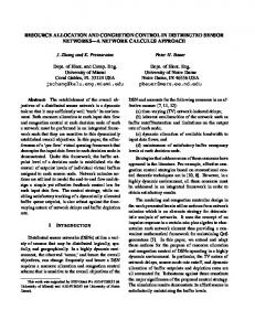
II. S YSTEM M ODEL Consider a downlink heterogeneous cellular network with 𝐼 multi-tier base stations (BSs) and 𝐽 users, as illustrated in Fig. 1. Let ℐ = {1, 2, ⋅ ⋅ ⋅ , 𝐼} and 𝒥 = {1, 2, ⋅ ⋅ ⋅ , 𝐽} be the set of all BSs and users, respectively. Denote 𝑥𝑖𝑗 as the association for BS 𝑖 and user 𝑗, i.e., 𝑥𝑖𝑗 = 1 when user 𝑗 is associated with BS 𝑖; otherwise, 𝑥𝑖𝑗 = 0. Assuming that each user is associated with only one BS, we have ∑ 𝑥𝑖𝑗 = 1, ∀𝑗 ∈ 𝒥 . (1)
Femto BS
Femto BS
Pico BS
Pico BS Macro BS
Femto BS
𝑖∈ℐ
In order to precisely characterize the inter-cell interference, we exploit the load and power coupled model, like in [10]. Denote 𝑦𝑖𝑗 as the fraction of resource allocated by BS 𝑖 for user 𝑗. Obviously, 𝑦𝑖𝑗 > 0 if and only if user 𝑗 is associated with BS 𝑖, which implies that 𝑦𝑖𝑗 ≤ 𝑥𝑖𝑗 . The load, 𝜌𝑖 , of BS 𝑖 can be evaluated by summing the fractions of resources occupied by users associated with BS 𝑖, i.e., ∑ 𝜌𝑖 = 𝑦𝑖𝑗 ≤ 1, ∀𝑖 ∈ ℐ. (2) 𝑗∈𝒥
Intuitively, the load proportion 𝜌𝑖 can also be interpreted as the probability of receiving interference from BS 𝑖 [10]. Denote 𝑝𝑖 as the transmission power of BS 𝑖. It is assumed that the transmission power of BS 𝑖 is the same for all users associated with BS 𝑖. The SINR of user 𝑗 associated with BS 𝑖 can be expressed as, 𝑝𝑖 𝑔𝑖𝑗 𝜂𝑖𝑗 1 = ∑ , (3) 2 𝑘∈ℐ∖{𝑖} 𝜌𝑘 𝑝𝑘 𝑔𝑘𝑗 + 𝜎 where 𝑔𝑖𝑗 is the channel gain (assuming constant and flatfading channel) from BS 𝑖 to user 𝑗 and 𝜎 2 represents the noise power. Then, the achievable rate, 𝑟𝑖𝑗 , of user 𝑗 associated with BS 𝑖 can be formulated as, 𝑟𝑖𝑗 = 𝑦𝑖𝑗 𝐵 log2 (1 + 𝜂𝑖𝑗 ),
(4)
where 𝐵 is the bandwidth of the network. Now it is ready to formulate the utility maximization problem as ( ) ∑ ∑ max 𝑈𝑗 𝑦𝑖𝑗 𝐵 log2 (1 + 𝜂𝑖𝑗 ) (5a) 𝑦 ,𝜌 𝜌,𝑝 𝑝 𝑥 ,𝑦
𝑗∈𝒥
𝑖∈ℐ
s.t. 𝜂𝑖𝑗 = ∑ ∑
𝑝𝑖 𝑔𝑖𝑗 , 2 𝑘∈ℐ∖{𝑖} 𝜌𝑘 𝑝𝑘 𝑔𝑘𝑗 + 𝜎
𝑥𝑖𝑗 = 1,
𝑖∈ℐ
𝜌𝑖 =
∑
𝑦𝑖𝑗 ,
∀𝑖 ∈ ℐ, ∀𝑗 ∈ 𝒥 (5b)
∀𝑗 ∈ 𝒥
(5c)
∀𝑖 ∈ ℐ
(5d)
𝑗∈𝒥
0 ≤ 𝑝𝑖 ≤ 𝑝max , 𝑖
∀𝑖 ∈ ℐ
0 ≤ 𝜌𝑖 ≤ 1, ∀𝑖 ∈ ℐ 0 ≤ 𝑦𝑖𝑗 ≤ 𝑥𝑖𝑗 , 𝑥𝑖𝑗 ∈ {0, 1},
(5e) ∀𝑖 ∈ ℐ, ∀𝑗 ∈ 𝒥
Fig. 1.
where 𝑥 = (𝑥11 , ⋅ ⋅ ⋅ , 𝑥1𝐽 , ⋅ ⋅ ⋅ , 𝑥𝐼𝐽 )𝑇 is the user association vector, 𝑦 = (𝑦11 , ⋅ ⋅ ⋅ , 𝑦1𝐽 , ⋅ ⋅ ⋅ , 𝑦𝐼𝐽 )𝑇 is the resource allocation vector, 𝜌 = (𝜌1 , ⋅ ⋅ ⋅ , 𝜌𝑁 )𝑇 is the load distribution vector, is 𝑝 = (𝑝1 , ⋅ ⋅ ⋅ , 𝑝𝑁 )𝑇 is the power control vector, and 𝑝max 𝑖 the maximal transmission power of BS 𝑖. In order to realize proportional fairness, we use the logarithmic utility function 𝑈𝑗 (𝑥) = log2 (𝑥), ∀𝑗 ∈ 𝒥 as in [8]. Since problem (5) is nonconvex, it is in general difficult to obtain the global optimum. In the following, we propose an iterative algorithm to solve this problem. III. I TERATIVE A LGORITHM In this section, we first provide the optimal condition for the load of each BS. Then, an iterative algorithm is proposed and the analysis of complexity is also provided. A. Optimal Condition for Load In order to facilitate the solution to problem (5), we here first present some interesting observations in the following Theorem 1 on the optimal strategy for BS loading. Note that this theorem can help us simplify the procedure of solving problem (5) without loss of optimality. Theorem 1: (5), the optimal load vector sat∑ For problem ∗ ∈ {0, 1}, ∀𝑖 ∈ ℐ, i.e., it is optimal for isfies 𝜌∗𝑖 = 𝑗∈𝒥 𝑦𝑖𝑗 each BS to operate at full load, i.e., 𝜌∗𝑖 = 1 or zero load, i.e., 𝜌∗𝑖 = 0. Proof : See Appendix A. Theorem 1 implies that the resource of a BS should be either fully used or shut down in order to maximize the network utility. This conclusion can be instructive for the actual operation of a HetNet. According to [8, Proposition 1], we can obtain the conclusion that the optimal resource allocation of problem (5) is equal allocation, i.e., 𝜌∗𝑖 𝑥∗𝑖𝑗 ∗ 𝑦𝑖𝑗 =∑ ∗ , 𝑙∈𝒥 𝑥𝑖𝑙
(5f) (5g)
1 If the resource allocation is randomly distributed, and we consider the long term average interference from other BSs, the SINR can somewhat be evaluated in (3).
System model.
where we define ∀𝑗 ∈ 𝒥 .
𝜌∗ 𝑥 ∗ ∑ 𝑖 𝑖𝑗 ∗ 𝑙∈𝒥 𝑥𝑖𝑙
(6)
= 0, for the case 𝜌∗𝑖 = 0, 𝑥∗𝑖𝑗 = 0,
B. Iterative User Association, Resource Allocation and Power Control Problem (5) is combinational due to the binary variable 𝑥𝑖𝑗 . Solving a combinational problem is usually impossible even for a modest-sized cellular network. We adopt the fractional user association relaxation in [8], where the association variables 𝑥𝑖𝑗 can take on any real value in [0,1]. Given optimal resource allocation in (6), the relaxation of problem (5) can be formulated as ( ) ∑∑ 𝐵𝜌𝑖 log2 (1 + 𝜂𝑖𝑗 ) ∑ (7a) 𝑥𝑖𝑗 log2 max 𝜌,𝑝 𝑝 𝑥 ,𝜌 𝑗∈𝒥 𝑥𝑖𝑗 𝑖∈ℐ 𝑗∈𝒥 𝑝𝑖 𝑔𝑖𝑗 s.t. 𝜂𝑖𝑗 = ∑ , ∀𝑖 ∈ ℐ, ∀𝑗 ∈ 𝒥 (7b) 2 𝑘∈ℐ∖{𝑖} 𝜌𝑘 𝑝𝑘 𝑔𝑘𝑗 + 𝜎 ∑ 𝑥𝑖𝑗 = 1, ∀𝑗 ∈ 𝒥 (7c) 𝑖∈ℐ
0 ≤ 𝜌𝑖 ≤ 1, ∀𝑖 ∈ ℐ 0 ≤ 𝑝𝑖 ≤ 𝑝max , ∀𝑖 ∈ ℐ 𝑖
(7d) (7e)
0 ≤ 𝑥𝑖𝑗 ,
(7f)
∀𝑖 ∈ ℐ, ∀𝑗 ∈ 𝒥
Now for the equivalently simplified problem in (7), we are able to present an iterative algorithm for solving the nonconvex problem. The idea is to develop a power control method with fixed user association for interference mitigation, and to design the user association method with fixed power in order to achieve better utility value. As long as both the power control and user association steps aim to increase the objective function (7a), the overall algorithm is guaranteed to converge. To solve the power control problem with fixed user association 𝑥 , we treat 𝜂𝑖𝑗 as new variables. Then, problem (7) with fixed 𝑥 is equivalent to the following problem : ∑∑ max 𝑥𝑖𝑗 log2 (𝜌𝑖 log2 (1 + 𝜂𝑖𝑗 )) (8a) 𝑝,𝜂 𝜂 𝜌 ,𝑝
𝑖∈ℐ 𝑗∈𝒥
s.t. 0 ≤ 𝜂𝑖𝑗 ≤ ∑
𝑝𝑖 𝑔𝑖𝑗 , ∀𝑖 ∈ ℐ, ∀𝑗 ∈ 𝒥 (8b) 2 𝑘∈ℐ∖{𝑖} 𝜌𝑘 𝑝𝑘 𝑔𝑘𝑗 + 𝜎
0 ≤ 𝜌𝑖 ≤ 1, ∀𝑖 ∈ ℐ 0 ≤ 𝑝𝑖 ≤ 𝑝max , ∀𝑖 ∈ ℐ 𝑖
(8c) (8d)
where 𝜂 = (𝜂11 , ⋅ ⋅ ⋅ , 𝜂1𝐽 , ⋅ ⋅ ⋅ , 𝜂𝐼𝐽 )𝑇 . If either one of 𝑝𝑖 and 𝜌𝑖 is 0, then the other is assumed to be 0. Based on this assumption, we have the following theorem. Theorem 2: If there exists at least one user 𝑗 such that 𝑥𝑖𝑗 = 1, the optimal 𝜌∗𝑖 of problem (8) is 𝜌∗𝑖 = 1; otherwise 𝜌∗𝑖 = 0. Proof : See Appendix B. According to Theorem 2, a BS should operate at full load if there exists at least one user associated to this BS, otherwise the BS would shut down, or equivalently with zero load. This is reasonable and straightforward, because it is always energy saving to shut off a BS if there is no user associated with this BS. Obviously, if 𝜌∗𝑖 = 0, we can obtain 𝑝∗𝑖 = 0 and 𝑥∗𝑖𝑗 = 0, ∀𝑗 ∈ 𝒥 . Thus, we only need to solve the power control problem for BSs with full load. Denote 𝒜 as the set of BSs with full load, i.e., 𝒜 = {𝑖 ∈ ℐ∣𝜌∗𝑖 = 1}. Owing to the fact
that each user is associated with one BS, there exists only one 𝑖 ∈ 𝒜 such that 𝑥𝑖𝑗 = 1 for any user 𝑗 ∈ 𝒥 . Let 𝒥𝑖 = {𝑗 ∈ 𝒥 ∣𝑥𝑖𝑗 = 1} denote the set of users associated with BS 𝑖. For notation convenience, we can use 𝜂𝑗 to replace 𝜂𝑖𝑗 , ∀𝑗 ∈ 𝒥𝑖 . Treating 𝜂𝑗 as new variables, problem (8) with optimal load distribution is equivalent to the following problem: ∑∑ max ln (ln(1 + 𝜂𝑗 )) (9a) 𝜂 𝑝 ,𝜂
𝑖∈𝒜 𝑗∈𝒥𝑖
s.t. 0 ≤ 𝜂𝑗 ≤ ∑
𝑝𝑖 𝑔𝑖𝑗 , ∀𝑖 ∈ 𝒜, 𝑗 ∈ 𝒥𝑖 (9b) 2 𝑘∈𝒜∖{𝑖} 𝜌𝑘 𝑝𝑘 𝑔𝑘𝑗 +𝜎
0 ≤ 𝑝𝑖 ≤ 𝑝max , 𝑖
∀𝑖 ∈ 𝒜
(9c)
𝑇
where 𝜂 = (𝜂1 , ⋅ ⋅ ⋅ , 𝜂𝐽 ) . Obviously, problem (9) is nonconvex due to constraints (9b). In the following, we use the exponential variable transformation, which has two advantages. One advantage is that the constraints 𝜂𝑗 ≥ 0 and 𝑝𝑖 ≥ 0 can be implicitly removed. The other advantage is that nonconvex constraints (9b) can be transformed into convex constraints and objective function (9a) remains concave after using exponential variable transformation. Due the above two advantages, the original nonconvex problem (9) can be transformed into a convex problem through exponential variable transformation. Then, the dual method can be used to obtain the optimal solution of problem (9). Let 𝜂𝑗 = e𝑢𝑗 and 𝑝𝑖 = e𝑣𝑖 , ∀𝑖 ∈ 𝒜, 𝑗 ∈ 𝒥𝑖 . Then, (9b) can be replaced by ∑ e𝑢𝑗 −𝑣𝑖 +𝑏𝑗 + e𝑢𝑗 +𝑣𝑘 −𝑣𝑖 +𝑎𝑘𝑗 ≤ 1, ∀𝑖 ∈ 𝒜, 𝑗 ∈ 𝒥𝑖 𝑘∈𝒜∖{𝑖}
(10) 2 𝜌 𝑔 where 𝑎𝑘𝑗 = ln 𝑘𝑔𝑖𝑗𝑘𝑗 , 𝑏𝑗 = ln 𝑔𝜎𝑖𝑗 , ∀𝑗 ∈ 𝒥𝑖 . Denote 𝑤𝑗 = 𝑢𝑗 −𝑣𝑖 +𝑏𝑗 , 𝑠𝑖𝑗 = 𝑢𝑗 +𝑣𝑖 −𝑣𝑘 +𝑎𝑘𝑗 , ∀𝑖, 𝑘 ∈ 𝒜, 𝑖 ∕= 𝑘, 𝑗 ∈ 𝒥𝑘 . Then, problem (9) is further equivalent to ∑∑ ln (ln(1 + e𝑢𝑗 )) (11a) max
𝑣 ,𝑤 𝑤 ,𝑠 𝑠 𝑢 ,𝑣
s.t.
𝑖∈𝒜 𝑗∈𝒥𝑖
e𝑤𝑗 +
∑
e𝑠𝑘𝑗 ≤ 1,
∀𝑖 ∈ 𝒜, 𝑗 ∈ 𝒥𝑖
(11b)
𝑘∈𝒜∖{𝑖}
𝑤𝑗 = 𝑢𝑗 − 𝑣𝑖 + 𝑏𝑗 , ∀𝑖 ∈ 𝒜, 𝑗 ∈ 𝒥𝑖 (11c) 𝑠𝑖𝑗 = 𝑢𝑗 + 𝑣𝑖 − 𝑣𝑘 + 𝑎𝑘𝑗 , ∀𝑖, 𝑘 ∈ 𝒜, 𝑖 ∕= 𝑘, 𝑗 ∈ 𝒥𝑘 (11d) max 𝑣𝑖 ≤ ln(𝑝𝑖 ), ∀𝑖 ∈ 𝒜 (11e) where 𝑢 = {𝑢𝑗 }𝑗∈𝒥 , 𝑣 = {𝑣𝑖 }𝑖∈𝒜 , 𝑤 = {𝑤𝑗 }𝑗∈𝒥 , 𝑠 = {𝑠𝑖𝑗 }𝑖,𝑘∈𝒜,𝑖∕=𝑘,𝑗∈𝒥𝑘 . Since e𝑢𝑗 (ln(1 + e𝑢𝑗 ) − e𝑢𝑗 ) ∂ 2 ln(ln(1 + e𝑢𝑗 )) = , 2 ∂𝑢𝑗 (1 + e𝑢𝑗 )2 ln2 (1 + e𝑢𝑗 ) and ln(1 + e𝑢𝑗 ) − e𝑢𝑗 < 0, the objective function (11a) is a concave function. Owing to the fact that constraints of problem (11) are all convex, problem (11) is a convex problem, which can be effectively solved by the well-established methods [16]. Instead of using the interior-point method, we adopt the dual method with low complexity to obtain the optimal solution of problem (11).
The Lagrangian function of problem (11) can be written by ∑∑ 𝑢, 𝑣 , 𝑤 , 𝑠 , 𝛼 , 𝛽 , 𝜆 , 𝜁 ) = ℒ (𝑢 ln (ln(1 + e𝑢𝑗 )) −
∑∑
𝑖∈𝒜 𝑗∈𝒥𝑖
⎛ 𝛼𝑗 ⎝e𝑤𝑗 +
𝑖∈𝒜 𝑗∈𝒥𝑖
−
∑∑
𝑖∈𝒜 𝑗∈𝒥𝑖
−
∑
∑
𝛽𝑗 (𝑤𝑗 − 𝑢𝑗 + 𝑣𝑖 − 𝑏𝑗 ) − ∑
1:
⎞ 2:
e𝑠𝑘𝑗 − 1⎠
𝑘∈𝒜∖{𝑖}
Algorithm 1 Iterative user association, resource allocation and power control (IURP) algorithm
∑
3:
𝜁𝑖 (𝑣𝑖 −
ln(𝑝max )) 𝑖
𝑖∈𝒜
𝜆𝑖𝑗 (𝑠𝑖𝑗 − 𝑢𝑗 − 𝑣𝑖 + 𝑣𝑘 − 𝑎𝑘𝑗 ),
(12)
4:
where 𝛼 = {𝛼𝑖 }𝑗∈𝒥 , 𝛽 = {𝛽𝑗 }𝑗∈𝒥 , 𝜆 = {𝜆𝑖𝑗 }𝑖,𝑘∈𝒜,𝑖∕=𝑘,𝑗∈𝒥𝑘 , and 𝜁 = {𝜁𝑖 }𝑖∈𝒜 . 𝛼 ≥ 0 , 𝛽 , 𝜆 and 𝜁 ≥ 0 are Lagrange multipliers associated with the corresponding constraints of problem (11). By using the dual method, the optimal solution of problem (11) can be obtained by iteratively optimizing primal vari𝑢, 𝑣 , 𝑤 , 𝑠 ) with fixed dual variables (𝛼 𝛼, 𝛽 , 𝜆 , 𝜁 ), and ables (𝑢 𝛼, 𝛽 , 𝜆 , 𝜁 )with fixed primal variables updating dual variables (𝛼 𝑢, 𝑣 , 𝑤 , 𝑠). To optimize the primary variables with fixed dual (𝑢 variables, we solve the KKT conditions. Given the optimized primary variables, we use the gradient method to update the dual variables. The details are given in Appendix C. Having solved the power control problem, we only need to obtain the optimal user association 𝑥 with fixed load distribution 𝜌 and power distribution 𝑝. With fixed 𝜌 and 𝑝, problem (7) becomes ( ) ∑∑ 𝐵𝜌𝑖 log2 (1 + 𝜂𝑖𝑗 ) ∑ 𝑥𝑖𝑗 log2 (13a) max 𝑥 𝑗∈𝒥 𝑥𝑖𝑗 𝑖∈ℐ 𝑗∈𝒥 ∑ 𝑥𝑖𝑗 = 1, ∀𝑗 ∈ 𝒥 (13b) s.t.
5:
𝑖,𝑘∈𝒜,𝑖∕=𝑘 𝑗∈𝒥𝑘
𝑖∈ℐ
0 ≤ 𝑥𝑖𝑗 ,
∀𝑖 ∈ ℐ, ∀𝑗 ∈ 𝒥
(13c)
Similar to the user association problem in [8], the optimal solution of problem (13) can be obtained by solving its dual problem with the gradient projection method. Numerical results in [8] show that the optimal 𝑥∗𝑖𝑗 of problem (13) is either 0 or 1, which indicates that every user is associated with at most one BS. Thus far, we are ready to present the iterative user association, resource allocation and power control (IURP) algorithm in Algorithm 1 to solve problem (7). C. Complexity Analysis We compare the computational complexity of the IURP algorithm with the existing iterative BS association and power control (IBAPC) algorithm [9]. For IBAPC algorithm, the main complexity lies in solving the power control problem (9) and user association problem (13). To solve subproblem (9), the complexity is 𝒪(𝐿NM 𝐼 2 ), where 𝐿NM is the average number of iterations by the classic Newton’s method [8]. To solve subproblem (13), the complexity is 𝒪(𝐿UA 𝐼𝐽) [8], where 𝐿UA is the average number of iterations by the gradient projection method [8]. Thus, the total complexity of IBAPC algorithm
Initialize any feasible 𝑥 (0) , the accuracy 𝜖, the iteration number 𝑛 = 1. Obtain the optimal 𝜌 (𝑛) of problem (8) with fixed 𝑥 (𝑛−1) through Theorem 2. 𝑢(𝑛) , 𝑣 (𝑛) , 𝑤 (𝑛) , 𝑠 (𝑛) ) with fixed Obtain the optimal (𝑢 (𝑛) (𝑛−1) 𝑥 by solving convex problem (11). Denote 𝑝𝑖 = (𝑛) (𝑛) e𝑣𝑖 for all 𝑖 ∈ 𝒜, and 𝑝𝑖 = 0 for all 𝑖 ∈ ℐ ∖ 𝐴. (𝑛) Obtain the optimal 𝑥 with fixed 𝜌 (𝑛) and 𝑝 (𝑛) by solving ∑ dual problem of (13). ∑ ∑ ∑ the If 𝑖∈ℐ 𝑗∈𝒥 ∣(𝑥(𝑛) − 𝑥(𝑛−1) )∣/ 𝑖∈ℐ 𝑗∈𝒥 𝑥(𝑛−1) < 𝜖, output 𝑥 ∗ = 𝑥 (𝑛) , 𝜌 ∗ = 𝜌 (𝑛) , 𝑝 ∗ = 𝑝 (𝑛) and terminate. Otherwise, set 𝑛 = 𝑛 + 1 and go to step 2.
is 𝑂(𝐿IB 𝐿NM 𝐼 2 + 𝐿IB 𝐿UA 𝐼𝐽), where 𝐿IB denotes the total number of outer iterations of the IBAPC algorithm. For the proposed IURP algorithm, the major complexity of the IURP algorithm also lies in solving two subproblems (11) and (13). To solve subproblem (11), we use the dual method to obtain the optimal power control by iteratively updating the primal variables and dual variables. To compute 𝑢𝑗 from (22) in Appendix C, we need to obtain the inverse function 𝑓 −1 (𝑥) with bisection method which has a complexity of 𝒪(log2 (1/𝜖0 )) for accuracy 𝜖0 . Then, the total complexity of solving subproblem (11) is 𝒪(𝐿DM 𝐼𝐽 log2 (1/𝜖0 ) + 𝐿DM 𝐼 2 𝐽), where 𝐿DM is the average number of iterations by dual method. For the interior point method, the complexity of solving (11) is 𝒪(𝐼 3 𝐽 3 ) [16]. Since iteration number 𝐿DM is usually smaller than user number 𝐽 from simulations, we can find that the dual method has a much lower complexity compared with the interior point method. Thus, the total complexity of the IURP algorithm is 𝒪(𝐿IU 𝐿DM 𝐼𝐽 log2 (1/𝜖0 ) + 𝐿IU 𝐿DM 𝐼 2 𝐽 + 𝐿IU 𝐿UA 𝐼𝐽), where 𝐿IU denotes the total number of outer iterations of the IURP algorithm. Obviously, the proposed IURP has a higher complexity compared with the IBAPC. However, the proposed IURP can yield the optimal power control with fixed user association, while only suboptimal power control with fixed user association is obtained by the IBAPC. IV. N UMERICAL R ESULTS We consider a three-tier HetNet with one macro BS (MBS), two pico BSs (PBSs) and two femto BSs (FBSs). The maximal transmission power of the three-tier HetNet is {46, 38, 30} dbm. We assume that there are a total number of 100 users uniformly distributed in the HetNet. The bandwidth is 𝐵 = 10 MHz, the noise power is 𝜎 2 = −104 dBm and the parameter 𝜒 in (23) of Appendix C is set as 10− 3. In modeling the propagation environment, we use a large-scale path loss 𝐿(𝑑) = 34 + 40 log(𝑑) and 𝐿(𝑑) = 37 + 30 log(𝑑) for MBS/PBSs and FBSs, respectively [8]. Besides, the standard deviation of shadow fading is set as 8 dB. We compare the proposed IURP algorithm with the IBAPC
60
1 0.9 0.8
Number of users served in each tier
MSINR−MP IBAPC IURP
CDF of rate
0.7 0.6 0.5 0.4 0.3 0.2
MBS PBSs FBSs
50
40
30
20
10
0.1 0
0
Fig. 2.
0
1
10 Rate (bits/s/Hz)
10
The CDF of overall rate in a three-tier HetNet.
Fig. 4.
IURP
The numbers of users per tier in a three-tier HetNet.
MBS PBSs FBSs
45
70
IBAPC IURP
40
60
35
50
Power /dBm
MSINR−MP
IBAPC
50
80
Utility−Utility
MSINR−MP
40 30
30 25 20 15
20
10
10
5
0 0
0 2
4
6
8
10
MSINR−MP
IBAPC
IURP
Iterations
Fig. 3.
Convergence behaviors of IBAPC and IURP.
algorithm, and the conventional max-SINR cell association with maximal transmission power (labeled as ‘MSINR-MP’). Fig. 2 shows the cumulative distribution function (CDF) of long-term rate in the HetNet with different user association and power control algorithms. From Fig. 2, the CDFs for IBAPC and IURP all improve significantly at low rate vs. MSINR-MP, showing a 3-4x gain. Moreover, we can find that the IURP always outperforms IBAPC. This is because the optimal solution of power control problem is obtained by solving an equivalent convex problem in IURP, and the suboptimal solution of power control problem is obtained by using the Newton’s method in IBAPC. In Fig. 3, we illustrate the convergence behaviors of IURP and IBAPC. It can seen that both IURP and IBAPC monotonically increase and converge rapidly. Obviously, the utility value by IURP outperforms IBAPC. This is because the optimal solution of power control problem is obtained in IURP, which requires more computations than IBAPC according to the complexity analysis in section III-C. Thus, we can conclude that the proposed algorithm achieves a significant performance gain at the cost of some additional computations. The average numbers of users per tier for different user
Fig. 5.
Optimized powers of per tier in a three-tier HetNet.
association and power control algorithms are shown in Fig. 4. It is observed that the algorithms with better performance tend to have larger number of users in PBSs and FBSs, which illustrates the benefit of off-loading traffic from the MBS to PBSs and FBSs. In addition, Fig. 5 shows the optimized powers of per tier for different user association and power control algorithms. We find that algorithms with better performance tend to have lower power in MBS and higher power in PBSs and FBSs. Combing Fig. 4 and Fig. 5, we conclude that a combination of setting MBS with lower power and smaller number of associated users is the key to obtaining good system performance. V. C ONCLUSION In this paper, we have investigated the logarithmic utility maximization problem for load-coupled HetNets. By analyzing the utility function, we prove that it is optimal for each BS to operate at full load or zero load. We propose an iterative algorithm, which consists of solving two subproblems: the power control problem and the user association problem. Although the power control problem with fixed user association is nonconvex, we transform it into an equivalent convex problem. The complexity of the proposed algorithm is also analyzed.
Simulation results show that the proposed algorithm achieves better performance than conventional schemes in terms of logarithmic utility. A PPENDIX A 𝑥∗ , 𝑦 ∗ , 𝜌 ∗ , Assume that the optimal solution of (5) is (𝑥 𝑝∑), where there exists at least one BS 𝑖 with 0 < 𝜌∗𝑖 = ∗ 𝑗∈𝒥 𝑦𝑖𝑗 < 1. Obviously, there exists at least one user 𝑗 ∗ > 0 and 𝑥∗𝑖𝑗 = 1 . Then, associated with BS 𝑖, i.e., 𝑦𝑖𝑗 we consider the following two cases of the value 𝜌∗𝑘 for all 𝑘 ∈ ℐ ∖ {𝑖}. 1) ∑ If 𝜌∗𝑘 = 0, ∀𝑘 ∈ ℐ ∖ {𝑖}. We choose 𝜖 > 0 such that ′ ∗ ′ ∗ + 𝜖 ≤ 1. Denote 𝑦𝑖𝑗 = 𝑦𝑖𝑗 + 𝜖. According to 𝜌𝑖 = 𝑗∈𝒥 𝑦𝑖𝑗 (3) and (4), we can obtain the achievable rate of user 𝑗 as ( ) 𝑝𝑖 𝑔𝑖𝑗 𝑟𝑖𝑗 = 𝑦𝑖𝑗 𝐵 log2 1 + ∑ . (14) 2 𝑘∈ℐ∖{𝑖} 𝜌𝑘 𝑝𝑘 𝑔𝑘𝑗 + 𝜎 𝑝∗
Based on (14), we have ( ) ( ) 𝑝∗𝑖 𝑔𝑖𝑗 𝑝∗𝑖 𝑔𝑖𝑗 ′ ′ ∗ 𝑟𝑖𝑗 = 𝑦𝑖𝑗 𝐵 log2 1 + 2 > 𝑦𝑖𝑗 𝐵 log2 1 + 2 . 𝜎 𝜎 (15) ′ ′ ′ , ⋅ ⋅ ⋅ , 𝑦1𝐽 , ⋅ ⋅ ⋅ , 𝑦𝐼𝐽 )𝑇 and 𝜌 ′ = (𝜌′1 , ⋅ ⋅ ⋅ , Denote 𝑦 ′ = (𝑦11 ′ ∗ ′ ∗ = 𝑦𝑘𝑙 , 𝑦𝑖𝑚 = 𝑦𝑖𝑚 , 𝜌′𝑘 = 𝜌∗𝑘 , ∀𝑘 ∈ ℐ ∖ 𝜌′𝑁 )𝑇 , where 𝑦𝑘𝑙 𝑥∗ , 𝑦 ′ , 𝜌 ′ , 𝑝 ∗ ), {𝑖}, 𝑙 ∈ 𝒥 , 𝑚 ∈ 𝒥 ∖ {𝑗}. With the new pair (𝑥 we can claim that the objective function (5a) is increased, 𝑥∗ , 𝑦 ∗ , 𝜌 ∗ , 𝑝 ∗ ) is the optimal which contradicts the fact that (𝑥 solution. In this case, we can obtain that 𝜌∗𝑖 = 1. 2) If there exists at least one BS 𝑘 ∈ ℐ ∖ {𝑖} such that 𝜌∗𝑘 > 0. According to (14), 𝑦𝑖𝑗 can be presented as 𝑦𝑖𝑗 =
𝑟𝑖𝑗 , 𝐵 log2 (1 + 𝑎𝑖𝑗 𝑝𝑖 )
(16)
𝑔
𝑖𝑗 where 𝑎𝑖𝑗 = ∑ 2. 𝑘∈ℐ∖{𝑖} 𝜌𝑘 𝑝𝑘 𝑔𝑘𝑗 +𝜎 ∗ ∗ With rate 𝑟𝑖𝑗 , load 𝜌𝑘 and power 𝑝∗𝑘 fixed, ∀𝑘 ∈ ℐ ∖ {𝑖}, we reduce the power 𝑝∗𝑖 to 𝑝′′𝑖 = 𝑝∗𝑖 − 𝜖′ , 𝜖′ > 0, which satisfies 𝑝′′𝑖 > 0. From (16), the corresponding resource allocation of ′′ ∗ = 𝑦𝑖𝑗 + 𝜖′′𝑗 , ∀𝑗 ∈ BS 𝑖 for user 𝑗 strictly increases to 𝑦𝑖𝑗 ′′ = 0, ∀𝑚 ∈∑{𝑙 ∈ 𝒥 ∣𝑦𝑖𝑙∗ = 0}. We {𝑙 ∈ 𝒥 ∣𝑦𝑖𝑙∗ > 0}. Let 𝑦𝑖𝑚 ′′ can choose a 𝜖′ > 0 such that 𝜌′′𝑖 = 𝑗∈𝒥 𝑦𝑖𝑗 ≤ 1. Denote ′′ ′′ ′′ ′′ 𝑇 ′′ ′′ 𝑦 = (𝑦11 , ⋅ ⋅ ⋅ , 𝑦1𝐽 , ⋅ ⋅ ⋅ , 𝑦𝐼𝐽 ) , 𝜌 = (𝜌1 , ⋅ ⋅ ⋅ , 𝜌′′𝑁 )𝑇 and ′′ ∗ = 𝑦𝑘𝑙 , 𝜌′′𝑘 = 𝜌∗𝑘 , 𝑝′′𝑘 = 𝑝∗𝑘 , 𝑝 ′′ = (𝑝′′1 , ⋅ ⋅ ⋅ , 𝑝′′𝑁 )𝑇 , where 𝑦𝑘𝑙 𝑥∗ , 𝑦 ′′ , 𝜌 ′′ , 𝑝 ′′ ), we ∀𝑘 ∈ ℐ ∖ {𝑖}, 𝑙 ∈ 𝒥 . With the new pair (𝑥 claim that (see the proof below) the objective function (5a) is increased. ∑ By contradiction, the optimal load vector must ∗ ∈ {0, 1}, ∀𝑖 ∈ ℐ. satisfy 𝜌∗𝑖 = 𝑗∈𝒥 𝑦𝑖𝑗 𝑟𝑖𝑗 𝑝𝑖 . Taking the Using (16), we obtain 𝑦𝑖𝑗 𝑝𝑖 = log (1+𝑎 𝑖𝑗 𝑝𝑖 ) 2 derivative of 𝑦𝑖𝑗 𝑝𝑖 with respect to (w.r.t.) 𝑝𝑖 yields
∑ ∂(𝑦𝑖𝑗 𝑝𝑖 )
(1 + 𝑎𝑖𝑗 𝑝𝑖 ) ln(1 + 𝑎𝑖𝑗 𝑝𝑖 ) − 𝑎𝑖𝑗 𝑝𝑖 . ∂𝑝𝑖 𝐵 ln2 (1 + 𝑎𝑖𝑗 𝑝𝑖 )(1 + 𝑎𝑖𝑗 𝑝𝑖 ) (17) It can be verified that the numerator of (17) is strictly increasing for 𝑝𝑖 ≥ 0. Since the numerator equals zero at 𝑝𝑖 = 0, the numerator is strictly positive for 𝑝𝑖 > 0. Thus ∂(𝑦𝑖𝑗 𝑝𝑖 )/∂𝑝𝑖 > 0. = ln(2)𝑟𝑖𝑗
Since power 𝑝∗𝑖 is reduced to 𝑝′′𝑖 = 𝑝∗𝑖 − 𝜖′ , 𝜖′ > 0, the ′′ ′′ ∗ ∗ ∗ 𝑝𝑖 is strictly than product 𝑦𝑖𝑗 ∑ smaller ∑𝑦𝑖𝑗 𝑝𝑖 , ∗∀𝑗∗∈ {𝑙 ∗∈ ∗𝒥 ∣𝑦𝑖𝑙 > ′′ ′′ ′′ ′′ 0}. Then, 𝜌𝑖 𝑝𝑖 = 𝑗∈𝒥 𝑦𝑖𝑗 𝑝𝑖 < 𝑗∈𝒥 𝑦𝑖𝑗 𝑝𝑖 = 𝜌𝑖 𝑝𝑖 . ∗ > 0, For any BS 𝑘 ∈ ℐ ∖ {𝑖} and user 𝑙 ∈ 𝒥 satisfying 𝑦𝑘𝑙 we have ( ) 𝑝′′𝑘 𝑔𝑘𝑙 ′′ ′′ 𝑟𝑘𝑙 = 𝑦𝑘𝑙 𝐵 log2 1 + ∑ ′′ ′′ 2 𝑛∈ℐ∖{𝑘} 𝜌𝑛 𝑝𝑛 𝑔𝑛𝑙 + 𝜎 ( ) 𝑝∗𝑘 𝑔𝑘𝑙 ∗ ∗ > 𝑦𝑘𝑙 𝐵 log2 1 + ∑ . (18) = 𝑟𝑘𝑙 ∗ 𝑝∗ 𝑔 + 𝜎 2 𝜌 𝑛𝑙 𝑛 𝑛 𝑛∈ℐ∖{𝑘} ∗ > 0, we have For BS 𝑖 and user 𝑗 ∈ 𝒥 satisfying 𝑦𝑖𝑗 ( ) 𝑝′′𝑖 𝑔𝑖𝑗 ′′ ′′ 𝑟𝑖𝑗 = 𝑦𝑖𝑗 𝐵 log2 1 + ∑ ′′ ′′ 2 𝑛∈ℐ∖{𝑖} 𝜌𝑛 𝑝𝑛 𝑔𝑛𝑙 + 𝜎 ( ) ∗ 𝑔 𝑝 𝑖𝑗 𝑖 ∗ ∗ = 𝑦𝑖𝑗 𝐵 log2 1 + ∑ , (19) = 𝑟𝑖𝑗 ∗ ∗ 2 𝑛∈ℐ∖{𝑖} 𝜌𝑛 𝑝𝑛 𝑔𝑛𝑙 + 𝜎 ′′ which can be proven through the derivation of 𝑝′′𝑖 and 𝑦𝑖𝑗 . Based on (18) and (19), we can prove that the the objective 𝑥∗ , 𝑦 ′′ , 𝜌 ′′ , 𝑝 ′′ ). function (5a) is increased with the new pair (𝑥
A PPENDIX B Assume that there exists one user 𝑗 such that 𝑥𝑖𝑗 = 1 and the optimal solution of problem (8) is 𝜌∗𝑖 ∕= 1. According to Theorem 1, 𝜌∗𝑖 ∈ {0, 1} and we have 𝜌∗𝑖 = 0. Denoting 𝜌′𝑖 = 1, we have 𝑥𝑖𝑗 log2 (𝜌∗𝑖 log2 (1 + 𝜂𝑖𝑗 )) = −∞ < 𝑥𝑖𝑗 log2 (𝜌′𝑖 log2 (1 + 𝜂𝑖𝑗 )), which contradicts the fact that 𝜌∗𝑖 is the optimal solution. Thus, we have 𝜌∗𝑖 = 1. Assume that 𝑥𝑖𝑗 = 0, ∀𝑗 ∈ 𝒥 and the optimal solution of problem (8) is 𝜌∗𝑖 ∕= 0. According to Theorem 1, 𝜌∗𝑖 ∈ {0, 1} and we have 𝜌∗𝑖 = 1. Let we set 𝜌′𝑖 = 0. For BS 𝑘 ∈ ℐ ∖ {𝑖} and user 𝑗 ∈ 𝒥 satisfying 𝑥𝑘𝑗 = 1, we have ( ( )) 𝑝𝑘 𝑔𝑘𝑗 ∗ 𝑥𝑘𝑗 log2 𝜌𝑘 log2 1 + ∑ ∗ 2 𝑛∈ℐ∖{𝑘} 𝜌𝑛 𝑝𝑛 𝑔𝑛𝑘 + 𝜎 ( ( )) 𝑝𝑘 𝑔𝑘𝑗 ∗ < 𝑥𝑘𝑗 log2 𝜌𝑘 log2 1 + ∑ , ∗ 2 𝑛∈ℐ∖{𝑖,𝑘} 𝜌𝑛 𝑝𝑛 𝑔𝑛𝑘 + 𝜎 which contradicts the fact that 𝜌∗𝑖 is the optimal solution. As a result, we have 𝜌∗𝑖 = 0. A PPENDIX C The optimal solution of problem (11) should satisfy the following KKT conditions [16]: ∑ 1 +𝛽𝑗 + 𝜆𝑖𝑗 = 0, ∀𝑗 ∈ 𝒥 (20a) 𝑢 𝑢 𝑗 𝑗 (1+e ) ln(1+e ) 𝑖∈𝒜∖{𝑘} ∑ ∑ ∑ ∑ ∑ − 𝛽𝑗 + 𝜆𝑖𝑗 − 𝜆𝑖𝑗 𝑗∈𝒥𝑖
𝑘∈𝒜∖{𝑖} 𝑗∈𝒥𝑘
− 𝜁𝑖 = 0, 𝑤𝑗
𝛼𝑗 e − 𝛽𝑗 = 0, 𝛼𝑗 e𝑠𝑖𝑗 −𝜆𝑖𝑗 = 0,
𝑘∈𝒜∖{𝑖} 𝑗∈𝒥𝑖
∀𝑖 ∈ ℐ ∀𝑗 ∈ 𝒥 ∀𝑖, 𝑘 ∈ 𝒜, 𝑖 ∕= 𝑘, 𝑗 ∈ 𝒥𝑘 .
(20b) (20c) (20d)
In the (𝑡 + 1)-th iteration of the dual method, we can calculate the primary variables with given the Lagrange multipliers 𝛼 (𝑡), 𝛽 (𝑡), 𝜆 (𝑡) and 𝜁 (𝑡). Based on (20a), for all 𝑗 ∈ 𝒥 , we have ∑ 1 𝜆𝑖𝑗 (𝑡) = − < 0. 𝛽𝑗 (𝑡) + 𝑢𝑗 (𝑡+1) ) ln(1 + e𝑢𝑗 (𝑡+1) ) (1 + e 𝑖∈𝒜 (21) Define function 𝑓 (𝑥) = (1 + e𝑥 ) ln(1 + e𝑥 ) and 𝑓 −1 (𝑥) is the inverse function of 𝑓 (𝑥), ∀𝑥 > 0. From (21), we have ( ) −1 −1 ∑ 𝑢𝑗 (𝑡 + 1) = 𝑓 , ∀𝑗 ∈ 𝒥 . (22) 𝛽𝑗 (𝑡) + 𝑖∈𝒜 𝜆𝑖𝑗 (𝑡) Since Lagrange function ℒ is a linear function w.r.t 𝑣𝑖 , the optimal value of 𝑣𝑖 can not be directly obtained. To solve this, we introduce a small positive constant 𝜒 > 0, and the objective function of problem (11a) can be modified as, ∑ ∑∑ max ln (ln(1 + e𝑢𝑗 ))+𝜒 ln(1+ln(𝑝max )−𝑣𝑖 ) 𝑖 𝑣 ,𝑤 𝑤 ,𝑠 𝑠 𝑢 ,𝑣
𝑖∈𝒜 𝑗∈𝒥𝑖
𝑖∈𝒜
(23) Obviously, the modified problem (11) with new objective function (23) is also a convex problem. Besides, if the value of 𝜒 is as small as possible, the optimal solution of the modified problem approximately equals to the optimal solution of original problem (11). By solving the KKT conditions of the modified problem, we can obtain )− 𝑣𝑖 (𝑡 + 1) = 1 + ln(𝑝max 𝑖 𝜒 ∑ ∑ ∑ ∑ − 𝛽𝑗 (𝑡)+ 𝜆𝑖𝑗 (𝑡)− 𝑗∈𝒥𝑖
𝑘∈𝒜∖{𝑖} 𝑗∈𝒥𝑘
∑
𝜆𝑖𝑗 (𝑡)−𝜁𝑖 (𝑡)
.(24)
𝑘∈𝒜∖{𝑖} 𝑗∈𝒥𝑖
To solve 𝑤 and 𝑠 , we first prove that 𝛼𝑗 (𝑡) ∕= 0 by using the contradiction method. If 𝛼𝑗 (𝑡) = 0, we have 𝛽𝑗 (𝑡) = 0 and ∑ 𝜆𝑖𝑗 (𝑡) = 0 according to (20c) and (20d). Thus, 𝛽𝑗 (𝑡) + 𝑖∈𝒜∖{𝑘} 𝜆𝑖𝑗 (𝑡) = 0, which contradicts (21). Due to the fact that 𝛼𝑗 (𝑡) ∕= 0, we can respectively obtain 𝑤𝑗 (𝑡 + 1) and 𝑟𝑖𝑗 (𝑡 + 1) from (20b) and (20c), ( ) 𝛽𝑗 (𝑡) 𝑤𝑗 (𝑡 + 1) = ln , ∀𝑗 ∈ 𝒥 . (25) 𝛼𝑗 (𝑡) ( ) 𝜆𝑖𝑗 (𝑡) 𝑠𝑖𝑗 (𝑡 + 1)=ln , ∀𝑖, 𝑘 ∈ 𝒜, 𝑖 ∕= 𝑘, 𝑗 ∈ 𝒥𝑘 . (26) 𝛼𝑗 (𝑡) To update the dual variables with the primal variables obtained from (22), (24)-(26), we exploit the gradient based method from [17]. The new value of the Lagrange multipliers is updated by ⎛ ⎞ ∑ e𝑠𝑘𝑗 (𝑡+1) −1⎠ 𝛼𝑗 (𝑡+1) =𝛼𝑗 (𝑡)+𝛿(𝑡)⎝e𝑤𝑗 (𝑡+1) + 𝑘∈𝒜∖{𝑖}
𝛽𝑗 (𝑡+1) = 𝛽𝑗 (𝑡)+𝛿(𝑡)(𝑤𝑗 (𝑡+1)−𝑢𝑗 (𝑡+1)+𝑣𝑖 (𝑡+1)−𝑏𝑗 ) 𝜆𝑖𝑗 (𝑡 + 1) = 𝜆𝑖𝑗 (𝑡)+𝛿(𝑡)(𝑠𝑖𝑗 (𝑡+1)−𝑢𝑗 (𝑡+1)−𝑣𝑖 (𝑡+1)+ 𝜁𝑖 (𝑡 + 1) = [𝜁𝑖 (𝑡) + 𝛿(𝑡)(𝑣𝑖 (𝑡+1) −
𝑣𝑘 (𝑡+1)−𝑎𝑘𝑗 ) + max ln(𝑝𝑖 ))]
where 𝛿(𝑡) is a dynamically chosen stepsize sequence, and [𝑥]+ denotes max{𝑥, 0}. A typical selection of 𝛿(𝑡) can be found in [17].
ACKNOWLEDGMENTS This work was supported by National 863 High Technology Development Project (No. 2014AA01A701), National Nature Science Foundation of China (Nos. 61471114, 61372106, & 61223001), Program Sponsored for Scientific Innovation Research of College Graduate in Jiangsu Province (No. KYLX15 0074), and Fundamental Research Funds for the Central Universities. R EFERENCES [1] J. G. Andrews, S. Buzzi, W. Choi, S. V. Hanly, A. Lozano, A. C. K. Soong, and J. C. Zhang, “What will 5g be?” IEEE J. Sel. Areas Commun., vol. 32, no. 6, pp. 1065–1082, June 2014. [2] J. T. Wang, “SINR feedback-based integrated base-station assignment, diversity, and power control for wireless networks,” IEEE Trans. Veh. Technol., vol. 59, no. 1, pp. 473–484, Jan. 2010. [3] L. Smolyar, I. Bergel, and H. Messer, “Unified approach to joint power allocation and base assignment in nonorthogonal networks,” IEEE Trans. Veh. Technol., vol. 58, no. 8, pp. 4576–4586, Oct. 2009. [4] S. Corroy, L. Falconetti, and R. Mathar, “Dynamic cell association for downlink sum rate maximization in multi-cell heterogeneous networks,” in Proc. IEEE Int. Conf. Commun. Ottawa, Canada, June 2012, pp. 2457–2461. [5] W. Yinghong, C. Yuan, X. Wei, and H. Nakamura, “Cell-specific association for heterogeneous networks with interference control,” IEICE Trans. on Commun., vol. 98, no. 4, pp. 653–660, 2015. [6] N. Wang, E. Hossain, and V. K. Bhargava, “Joint downlink cell association and bandwidth allocation for wireless backhauling in two-tier hetnets with large-scale antenna arrays,” 2015. [Online]. Available: http://arxiv.org/abs/1501.00078 [7] X. Zhou, S. Feng, Z. Han, and Y. Liu, “Distributed user association and interference coordination in HetNets using Stackelberg game,” in Proc. IEEE Int. Conf. Commun. London, UK, June 2015, pp. 6431–6436. [8] Q. Ye, B. Rong, Y. Chen, M. Al-Shalash, C. Caramanis, and J. G. Andrews, “User association for load balancing in heterogeneous cellular networks,” IEEE Trans. Wireless Commun., vol. 12, no. 6, pp. 2706– 2716, June 2013. [9] K. Shen and W. Yu, “Distributed pricing-based user association for downlink heterogeneous cellular networks,” IEEE J. Sel. Areas Commun., vol. 32, no. 6, pp. 1100–1113, June 2014. [10] I. Siomina and D. Yuan, “Analysis of cell load coupling for LTE network planning and optimization,” IEEE Trans. on Wireless Commun., vol. 11, no. 6, pp. 2287–2297, June 2012. [11] A. J. Fehske and G. P. Fettweis, “Aggregation of variables in load models for interference-coupled cellular data networks,” in Proc. IEEE Int. Conf. Commun. (ICC). Ottawa, Canada, June 2012, pp. 5102–5107. [12] I. Siomina and D. Yuan, “On constrained cell load coupling with applications in LTE networks,” IEEE Commun. Lett., vol. 18, no. 10, pp. 1771–1774, Oct. 2014. [13] ——, “On optimal load setting of load-coupled cells in heterogeneous LTE networks,” in Proc. IEEE Int. Conf. Commun. (ICC). Sydney, Australia, June 2014, pp. 1254–1259. [14] X. Chen, C. Wu, Y. Zhou, and H. Zhang, “A learning approach for traffic offloading in stochastic heterogeneous cellular networks,” in Proc. IEEE Int. Conf. Commun. (ICC). London, UK, June 2015, pp. 3347–3351. [15] L. You and D. Yuan, “Load optimization with user association in cooperative and load-coupled LTE networks,” 2016. [Online]. Available: http://arxiv.org/abs/1602.07255 [16] S. Boyd and L. Vandenberghe, Convex Optimization. Cambridge University Press, 2004. [17] D. P. Bertsekas, Convex Optimization Theory. Athena Scientific Belmont, 2009.