USING A GENETIC ALGORITHM TO LEARN BEHAVIORS FOR AUTONOMOUS VEHICLES† Alan C. Schultz and John J. Grefenstette Navy Center for Applied Research in Artificial Intelligence (Code 5514), Naval Research Laboratory, Washington, DC 20375-5000, U.S.A. EMAIL:
[email protected] (202) 767-2684 nomous vehicle, both projective planning and reactive components will be necessary and recently, researchers have been examining systems that combine both projective and reactive elements in order to exploit the strengths of both systems (Arkin,1989; Laird, et al, 1991).
Abstract Truly autonomous vehicles will require both projective planning and reactive components in order to perform robustly. Projective components are needed for long-term planning and replanning where explicit reasoning about future states is required. Reactive components allow the system to always have some action available in real-time, and themselves can exhibit robust behavior, but lack the ability to explicitly reason about future states over a long time period. This work addresses the problem of creating reactive components for autonomous vehicles. Creating reactive behaviors (stimulus-response rules) is generally difficult, requiring the acquisition of much knowledge from domain experts, a problem referred to as the knowledge acquisition bottleneck. SAMUEL is a system that learns reactive behaviors for autonomous agents. SAMUEL learns these behaviors under simulation, automating the process of creating stimulus-response rules and therefore reducing the bottleneck. The learning algorithm was designed to learn useful behaviors from simulations of limited fidelity. Current work is investigating how well behaviors learned under simulation environments work in real world environments. In this paper, we describe SAMUEL, and describe behaviors that have been learned for simulated autonomous aircraft, autonomous underwater vehicles, and robots. These behaviors include dog fighting, missile evasion, tracking, navigation, and obstacle avoidance.
Projective (or deliberative) components are needed for long-term planning and replanning where explicit reasoning about future states is required. One problem with projective systems are that they are unnecessarily slow on tasks that are performed often. That is, they generally must rethink solutions to problems that are seen over and over again. Also, projective systems usually require a model over which the reasoning takes place. Real-time performance is often a critical requirement for many of the capabilities needed in autonomous vehicles. Reactive systems in which stimulus-response rules drive the behavior of the vehicle easily achieve real-time performance and can perform well in a wide variety of situations. Furthermore, reactive systems typically require no underlying model. The weakness of reactive systems is the inability to explicitly reason about future states over long periods of time. This allows the reactive system to occasionally get into situations that they cannot resolve. An interesting problem in the design of intelligent, autonomous systems is the creation of the projective and reactive components. In this paper, we consider the creation of the reactive component. Creating reactive behaviors (stimulus-response rules) is generally difficult, requiring the acquisition of knowledge from domain experts, a problem referred to as the knowledge acquisition bottleneck. This paper presents work on S AMUEL, a system that learns reactive behaviors for autonomous agents. S AMUEL, based on genetic algorithms (Holland, 1975), learns these behaviors under simulation, automating the process of creating stimulus-response rules and therefore
1. Introduction As hardware issues are being resolved, and as competent low-level controllers are being designed, attention in autonomous vehicle design is now focusing more on the higher level autonomic functions of these vehicles. Historically, many researchers have examined either projective planning (e.g. Kanade, 1990) or reactive systems (e.g. Brooks, 1991) in isolation for control of an autonomous vehicle. However, in order to create a truly robust, intelligent auto__________________
† In Proceedings of the AIAA Guidance, Navigation and Control Conference, Hilton Head, SC, August 10-12, 1992.
1
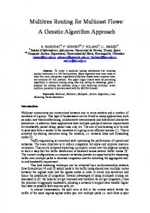
ON-LINE SYSTEM
TARGET ENVIRONMENT
OFF-LINE SYSTEM
RULE INTERPRETER
SIMULATION MODEL
RULE INTERPRETER
ACTIVE BEHAVIOR
LEARNING MODULE
TEST BEHAVIOR
Fig. 1. A Model for Learning from a Simulation Model. reducing the bottleneck. The learning algorithm was designed to learn useful behaviors from simulations of limited fidelity. The expectation is that behaviors learned in these simulations will be useful in realworld environments. Previous studies have illustrated that knowledge learned under simulation is robust and might be applicable to the real world if the simulation is more general (i.e. has more noise, more varied conditions, etc.) than the real world environment (Ramsey, Schultz and Grefenstette, 1990), and work continues in this area.
the population of behaviors. In Section 2, the SAMUEL system and one domain will be described. This domain is introduced to describe the SAMUEL system in context. Section 3 will describe other autonomous vehicle domains and results from learning in these domains. Section 4 will describe related ongoing and future research. 2. Description of the SAMUEL System SAMUEL is a system designed to learn reactive behaviors for solving sequential decision problems. SAMUEL consists of three major components: a problem specific module, a performance module, and a learning module. Figure 2 shows the architecture of the system. The problem specific module consists of the world model and its interfaces. In these experiments, the world model is a simulation of an autonomous vehicle its environment. The performance module is called CPS (Competitive Production System), a production system that interacts with the world model by reading sensors, setting control variables, and obtaining payoff from a critic. Like traditional production system interpreters, CPS performs matching and conflict resolution. In addition, CPS performs rule-level assignment of credit based on the intermittent feedback from the critic. The learning module uses a genetic algorithm to develop reactive behaviors, expressed as a set of condition-action rules. Each behavior is evaluated by testing its performance on a number of tasks in the world model. As a result of these evaluations, behaviors are selected for replication and modification. Genetic operators, such as crossover and mutation, and other operators, such as generalization and specialization, produce plausible new behaviors from high performance precursors.
The approach described here reflects a particular methodology for learning via a simulation model. The motivation is that making mistakes on real systems may be costly or dangerous. In addition, time constraints might limit the number of experiences during learning in the real world, while in many cases, the simulation model can be made to run faster than real time. Since learning may require experimenting with behaviors that might occasionally produce unacceptable results if applied to the real world, or might require too much time in the real environment, we assume that hypothetical behaviors will be evaluated in a simulation model (see Figure 1). Genetic algorithms, the heart of SAMUEL, are powerful, adaptive search techniques that can learn high performance knowledge structures. The genetic algorithm’s strength comes from the implicitly parallel search of the solution space that it performs, via a population of candidate solutions. In SAMUEL, the population is composed of candidate reactive behaviors for solving the problem. S AMUEL evaluates the candidate behaviors by testing them in a simulated environment. Based on the behaviors’ overall performance in this environment, genetic and other operators are applied to improve the performance of
2
PROBLEM SPECIFIC MODULE
WORLD MODEL
PERFORMANCE (CPS) MODULE
SENSORS
MATCHER
CONTROLS
CONFLICT RESOLUTION
CRITIC
CREDIT ASSIGNMENT
CURRENT BEHAVIOR
BEHAVIOR FITNESS CURRENT BEST BEHAVIOR
RULE STRENGTHS COMPETING BEHAVIORS
GENETIC ALGORITHM NEW BEHAVIOR
LEARNING MODULE
Fig. 2. SAMUEL: A Learning System for Reactive Behaviors
2.1. Problem Specific Module: Description of AUV simulation domain
2.1.1. Sensors We assume that the AUV knows its own position with some margin of error, and that the position of the stationary target is known, again with some margin of error. The AUV is equipped with an active sonar for detecting obstacles in its path. The sonar is composed of seven cells, each with a resolution of 10 degrees, giving the AUV a total coverage of 70 degrees. The AUV also has some internal, or virtual, sensors that give the AUV certain information about its own state. The sensors are:
To illustrate the problem specific module and the other modules of the system, we now describe one autonomous vehicle domain under study, collision avoidance and navigation for an autonomous underwater vehicle (AUV). In this domain, we have a simple two-dimensional simulation of an AUV that must navigate through a dense mine field towards a stationary object with which it must rendezvous. The AUV has a limited set of sensors, including sonar, and must set its speed and direction each decision cycle. We wish to learn a reactive behavior that is expressed as a set of reactive rules, (i.e. stimulus-response rules) that map sensor readings to actions to be performed at each decision time-step. Note that the system does not learn a specific path, but a set of rules that reactively decide a move at each time step allowing the vehicle to reach its goal and avoid the mines.
3
last-turn:
The current turning rate of the AUV. This sensor can assume 13 values, ranging from -60 degrees to 60 degrees in 10 degree increments.
time:
The current elapsed time, an integer.
range:
The range to the rendezvous area. Assumes 16 values from 0 to 1500.
bearing:
The bearing to the rendezvous area. Assumes integer values from 1 to 12.
speed:
The bearing is expressed in ‘‘clock terminology’’, in which 12 o’clock denotes dead ahead of the AUV.
depending on the AUV’s distance from the goal when the AUV is lost; this gives partial credit for failures.
The current speed of the AUV. Assumes 9 values from 0 to 40. Note that the AUV can come to a stop.
2.2. Performance Component The performance module of SAMUEL, CPS, has some similarities to both traditional production system interpreters and to classifier systems. The primary features of CPS are a restricted but high level rule language, partial matching, competition-driven conflict resolution, and incremental credit assignment methods. These features are described in more detail in the following sections.
asonar_n: One of 7 active sonar cells used for collision avoidance. Each cell takes on values from 0 to 200 in increments of 10 (20 bins) and represents the distance to an object within that sonar cell’s view. If no object is seen, a special value indicates that no object is sensed.
2.2.1. Knowledge Representation
Each sensor can have noise added to simulate a more realistic environment. In particular, the sonar readings have both a gaussian noise added, and a small random probability of "missing" an object, or of reading a "ghost" object that is not really there.
In a departure from many previous genetic learning systems, SAMUEL learns rules expressed in a high level rule language. The use of a high level language for rules offers several advantages over low level binary pattern languages typically adopted in genetic learning systems. First, it is easier to incorporate existing knowledge, whether acquired from experts or by symbolic learning programs. Second, it is easier to explain the knowledge learned through experience. Each CPS rule has the form
2.1.2. Actions (effectors) There is a discrete set of actions available to control the AUV. In this study, we consider actions that specify discrete turning rates and discrete speeds for the AUV. The control variable turn has 13 possible settings, between -30 and 30 degrees in five degree increments. The control variable speed has 9 possible settings between 0 and 40 (the units are arbitrary) with an increment of five. The learning objective is to develop a reactive plan, i.e., set of decision rules that map current sensor readings into actions, that successfully allows the AUV to rendezvous with the stationary target without using up all of its fuel while avoiding mines.
IF c1 THEN a 1
B
1.0,
if AUV reaches goal area
50 / (50 + range),
otherwise.
AND AND
cn am
The form of the conditions depends on the type of the sensor. SAMUEL supports four types of sensors: linear, cyclic, structured, and pattern. Linear sensors take on linearly ordered numeric values. Conditions over linear sensors specify upper and lower bounds for the sensor values. For example, the speed sensor in AUV can take on values over the range 0 to 40, discretized into 8 equal segments. Thus, an example of a legal condition over speed is speed is [10 .. 15]
which matches if 10 ≤ speed ≤ 15. In AUV, last-turn, time, range, speed, and the sonar cells are linear sensors. Cyclic sensors take on cyclicly ordered numeric values. Like linear sensors, the range of each cycle sensor is divided by the user into equal segments whose endpoints constitute the legal bounds in the conditions. Unlike linear sensors, any pair of legal values can be interpreted as a valid condition for cyclic sensors. In AUV, bearing is a cyclic sensor, since the next ‘‘higher’’ value than bearing = 12 is
C D
. . . . . .
where each ci is a condition on one of the sensors and each action a j specifies a setting for one of the control variables.
The AUV simulation is divided into episodes that begin with the placement of the AUV centered in front of a randomly generated mine field with a specified density. The episodes end with either a successful rendezvous at the target location, or a loss of the AUV due to time running out (no fuel) or a collision with a mine. The rendezvous is successful if the AUV approaches within 50 units of the target location. It is assumed that the only feedback provided is a numeric payoff, supplied at the end of each episode, that reflects the success of the episode with respect to the goal of reaching the rendezvous point. The payoff is defined by the formula: payoff =
AND AND
The payoff returned by the critic is 1.0 for a success and a value between 0 and 0.5 (non-inclusive)
4
bearing = 1.
2.3. The Learning Module
The rule language of CPS also supports structured nominal sensors whose values are taken from the nodes of a tree-structured hierarchy. Conditions for structured sensors specify a list of values, and the condition matches if the sensor’s current value occurs in a subtree labeled by one of the values in the list. Structured nominal sensors are not used in the AUV domain, but that are used in the other three domains presented.
Learning in SAMUEL occurs on two distinct levels: credit assignment at the rule level, and genetic competition at the plan level. 2.3.1. Credit Assignment Systems that learn rules for sequential behavior generally face a credit assignment problem: If a sequence of rules fires before the system solves a particular problem, how can credit or blame be accurately assigned to early rules that set the stage for the final result? Our approach is to assign each rule a measure called strength that serves as a prediction of the expected level of payoff that will be achieved if this rule fires. When payoff is obtained at the end of an episode, the strengths of all active rules (i.e., rules that suggested the actions taken during the current episode) are incrementally adjusted to reflect the current payoff. The adjustment scheme, called the Profit Sharing Plan (PSP), consists of subtracting a fraction of the rule’s current strength and adding the same fraction of the payoff. Rules whose strength correctly predicts the payoff retain their original levels of strength, while rules that overestimate the expected payoff lose strength and rules that underestimate payoff gain strength. However, conflict resolution should take into account not only the expected payoff associated with each rule, but also some measure of our confidence in that estimate. One way to measure confidence is through the variance associated with the estimated payoff. In SAMUEL, the PSP has been adapted to estimate both the mean and the variance of the payoff associated with each rule. Thus, a high strength rule must have both high mean and low variance in its estimated payoff. By biasing conflict resolution toward high strength rules, we expect to select actions for which we have high confidence of success.
The right-hand side of each rule specifies a setting for one or more control variables. For the AUV problem, each rule specifies a setting for the variable turn, and a setting for the variable speed. In general, a given rule may specify conditions for any subset of the sensors and actions for any subset of the control variables. Each rule also has a numeric strength, that serves as a prediction of the rule’s utility (Grefenstette, 1988). The methods used to update the rule strengths is described in the section on credit assignment below. 2.2.2. Production System Cycle CPS follows the match/conflict-resolution/act cycle of traditional production systems. Since there is no guarantee that the current set of rules is in any sense complete, it is important to provide a mechanism for handling cases in which no rule matches. In CPS this is accomplished by assigning each rule a match score equal to the number of conditions it matches. The match set consists of all the rules with the highest current match score. Once the match set is computed, an action is selected from the (possibly conflicting) actions recommended by the members of the match set. Each possible action receives a bid equal to the strength of the strongest rule in the match set that specifies that action in its right-hand side. CPS selects an action using the probability distribution defined by the strength of the (single) bidder for each action. This prevents a large number of low strength rules from combining to suggest an action that is actually associated with low payoff. All rules in the match set that agree with the selected action will have their strength adjusted according to the credit assignment algorithm described in the next section.
2.3.2. The Genetic Algorithm At the plan level, SAMUEL treats the learning process as a heuristic optimization problem, i.e., a search through a space of knowledge structures looking for structures that lead to high performance. A genetic algorithm is used to perform the search. Genetic algorithms are motivated by standard models __________________
After conflict resolution, the control variables are set to the values indicated by the selected actions.1 The world model is then advanced by one simulation step. The new state is reflected in a new set of sensor readings, and the entire process repeats.
1 If there is more than one control variable, as is the case in the AUV domain, the conflict resolution phase is executed independently for each control variable. As a result, the settings for different control variables may be recommended by distinct rules.
5
of heredity and evolution in the field of population genetics, and embody abstractions of the mechanisms of adaptation present in natural systems (Holland, 1975). Briefly, a genetic algorithm simulates the dynamics of population genetics by maintaining a knowledge base of knowledge structures that evolves over time in response to the observed performance of its knowledge structures in their training environment. Each knowledge structure yields one point in the space of alternative solutions to the problem at hand, which can then be subjected to an evaluation process and assigned a measure of fitness reflecting its potential worth as a solution. The search proceeds by repeatedly selecting structures from the current knowledge base on the basis of fitness, and applying idealized genetic search operators to these structures to produce new structures (offspring) for evaluation. Goldberg (1989) and Davis (1991) provide a detailed discussion of genetic algorithms. The learning level of SAMUEL is a specialized version of a standard genetic algorithm, GENESIS (Grefenstette, 1986). In SAMUEL, the knowledge structures that make up the population are behaviors, or sets of reactive rules, that represent a strategy for solving the problem. The remainder of this section outlines the differences between GENESIS and the genetic algorithm in SAMUEL.
random, e.g. the location of the mines and the goal location. In order to introduce plausible new rules, (and also to specialize overly general rules in the plan later in the learning) a plan modification operator called SPECIALIZE is applied after each evaluation of a plan. This operator will trigger if there is room in the plan for at least one more rule. and an episode ended with a successful rendezvous. SPECIALIZE creates
a new rule with the right hand side being set to the action that occurred during the successful episode that triggered the operator, and with a more specialized left-hand side. For each sensor, the condition for the sensor in the new rule covers approximately half the legal range for that sensor, splitting the difference between the extreme legal values and the sensor reading obtained from the successful episode. For example, suppose the initial plan contains the maximally general rule: IF THEN turn is ANY AND speed is ANY
Suppose further that the following step is recorded in the evaluation trace during the evaluation of this plan: . . . sensors: ... time = 4, range = 500, bearing = 6 ... action: turn = -15, speed = 10 . . .
2.3.2.1. Adaptive Initialization and Using Existing Knowledge Several approaches to initializing the knowledge structures of a genetic algorithm have been reported. By far, random initialization of the first population is the most common method. This approach requires the least knowledge acquisition effort, provides a lot of diversity for the genetic algorithm to work with, and presents the maximum challenge to the learning algorithm. As a second alternative, we have developed an approach called adaptive initialization. Each plan starts out as a completely general rule, but its rule is specialized according to its early experiences, thus creating more rules for each plan. Specifically, each plan in the initial population consists of a maximally general rule which says:
Then SPECIALIZE would create the following new rule: IF
time is [2 .. range is [300 bearing is [3 ... THEN turn is [-15]
11] AND .. 1000] AND .. 9] AND AND speed is [10]
The resulting rule is given a high initial strength, and added to the plan. The new rule is plausible, since its action is known to be successful in at least one situation that matches its left hand side. Of course, the new rule is likely to need further modification, and is subject to further competition with the other rules.
for any sensor readings, take any action A plan consisting of only this rule executes a random walk, since the rule matches on every cycle and specifies any possible legal action. Although each plan in the initial population executes this random walk policy, it does not follow that they all have the same performance, since the initial conditions for the episodes used to evaluate the plans are selected at
A third approach is to seed the initial population with existing knowledge (Schultz and Grefenstette, 1990). The rule language of SAMUEL was designed to facilitate the inclusion of available knowledge. In some cases, such as the AUV domain, random behavior will never yield a success and so the
6
adaptive initialization will not have sufficient information for adequately specializing the maximally general rule. In these domains, it is essential that the initial population include heuristic knowledge to start the search. This initial knowledge does not need to lead to very good results, but simply gives the system some initial successes so that the adaptive initialization will work. Following are the set of initial rules used in this study. Note that the performance achieved with this hand-crafted plan is only eight percent, i.e. the AUV can successfully reach the rendezvous area 8 out of 100 episodes. Note that this plan does not specify any action values for the speed action; they must be learned.
2.3.2.3. Selection Plans are selected for reproduction on the basis of their overall fitness scores returned by CPS. Using the notion of "survival of the fittest", plans that perform well get to produce more offspring (i.e. plans) for the next generation. The topic of reproductive selection in genetic algorithms is discussed in the literature (De Jong, 1975; Goldberg, 1989). In SAMUEL, the fitness of each plan is defined as the difference between the average payoff received by the plan and some baseline performance measure. The baseline is adjusted to track the mean payoff received by the population, minus one standard deviation. The baseline is adjusted slowly to provide a moderately consistent measure of fitness. Plans whose payoff fall below the baseline are assigned a fitness measure of 0, resulting in no offspring. This mechanism appears to provide a reasonable way to maintain consistent selective pressure toward higher performance.
# Goal is somewhat in front of us; nothing # is too close ahead, go straight IF bearing is [11 .. 1] AND asonar4 is [180 .. INF] THEN turn is [0] # Goal is somewhat is front of us; object # within range in front of us; turn hard. IF bearing is [11 .. 1] AND asonar4 is [10 .. 190] THEN turn is [30]
2.3.2.4. Genetic Operators Selection alone merely produces clones of high performance plans. CROSSOVER works in concert with selection to create plausible new plans. In SAMUEL, CROSSOVER treats rules as indivisible units. Since the rule ordering within a plan is irrelevant, the process of recombination can be viewed as simply selecting rules from each parent to create an offspring plan. In SAMUEL, CROSSOVER assigns each rule in two selected parent plans to one of two offspring plans. CROSSOVER attempts to cluster rules that are temporally related before assigning them to offspring. The idea is that rules that fire in sequence to achieve a successful rendezvous should be treated as a group during recombination, in order to increase the likelihood that the offspring plan will inherit some of the better behavior patterns of its parents. Of course, the offspring may not behave identically to either one of its parents, since the probability that a given rule fires depends on the context provided by all the other rules in the plan. The effect is that small groups of rules that are associated with high performance propagate through the population of plans, and serve as building blocks for new plans.
# Turn towards the goal. IF bearing is [2 .. 6] THEN turn is [-30] IF bearing is [6 .. 10] THEN turn is [30] # A maximally general rule. # Choose speed randomly. IF THEN speed is ANY
2.3.2.2. Evaluation Each plan is evaluated by invoking CPS, using the given plan as rule memory. CPS executes a fixed number of episodes, and returns the average payoff as the fitness for the plan. The updated strengths of the rules are also returned to the learning module. Each episode begins with randomly selected initial conditions, and thus represents a single sample of the performance of the plan on the space of all possible initial condition of the world model. Earlier work indicated that it is important for the simulation model to include more variability and noise that the actual environment (Grefenstette, Ramsey and Schultz, 1990). In this study, noise is included in the sensors, and each initial environment is comprised of a random mine field.
While CROSSOVER operates on the entire population of plans, recombining rules among the plans, SAMUEL also includes six unary operators that modify the rules within a single behavior: MUTATION, CREEP, SPECIALIZE, GENERALIZE, MERGE, and DELETE. Unlike previous versions of the system, SAMUEL has now adopted the policy that all of these operators except DELETE are creative. All modifications are made on a
7
new copy of the original rule, and the altered rule is added into the plan, where it will compete at the rule level with the rule from which it was created. A rule survives intact unless it is explicitly deleted or lost when its behavior is not selected for reproduction. This policy allows a much more aggressive application of rule modification operators with little damage if the changes are maladaptive. Each of these operators will now be discussed.
3. Results and Other Domains This section will describe the results from the collision avoidance and navigation domain and then briefly describe and give results of three other domains for which behaviors have been learned. Each of these domains represent behaviors that are important to an autonomous vehicle whether the vehicle is an air vehicle, land vehicle or underwater vehicle. The three additional domains are tracking, dog fighting, and missile evasion.
The genetic operator MUTATION introduces a new rule by making random changes to a copy of an existing rule. For example, MUTATION might alter a condition within a rule from asonar_4 [150 .. 200] to asonar_4 [10 .. 200]. The operator CREEP is similar to MUTATION, except that it only makes small changes, e.g. from asonar_4 [150 .. 200] to asonar_4 [140 .. 200]. This operator ‘‘creeps’’ a value the smallest increment possible for a particular sensor or action.
3.1. Results from Navigation Avoidance Domain
and Obstacle
Simulation results demonstrate that an initial, human-designed behavior which has an average success rate of only eight percent on randomly generated mine fields can be improved by this system so that the final behavior can achieve a success rate of 96 percent.
The SPECIALIZE operator was described earlier in Section 2.3.2.1 during the discussion of population initialization. This operator is applied when general rules fire in successful episodes. The operator creates a new rule whose left hand side more closely matches the sensor values existing at the time the general rule fired, and whose right hand side more closely matches the action that was actually taken.
The experiments shown here reflect our assumptions about the methodology of simulationassisted learning. At periodic intervals (10 generations in the current experiments), a single behavior is extracted from the current population to represent the learning system’s current hypothetical behavior. This behavior is tested for 100 randomly chosen problem episodes. The assumption is that the current best behavior can be extracted from the learning system and used in the real world while the learning system continues looking for a better hypothesis.
The GENERALIZE operator creates rules that are more general versions of overspecialized rules. GENERALIZE can be applied when a rule fires because of a partial match during a successful episode. A partial match occurs when no rule fully matches the current sensors, and the rule that most closely matches is selected. This operator creates a rule that will match when a similar situation occurs again by generalizing the conditions enough to match the sensor readings that were active when the rule fired.
In the first experiment, the system was initialized with the rules discussed and shown in section 2.3.2.1. Each episode, the AUV was placed centered before a randomly generated mine field with a density of 25 mines. The rendezvous area was placed at a random point on the other side of the mine field. SAMUEL was then run for 100 generations. Each evaluation of a behavior is the average over 20 episodes, as discussed earlier. Since a stochastic process is involved, each experiment was repeated ten times, and the results averaged. Before learning, with just the initial rules by themselves, the AUV will rendezvous with the goal just eight out of 100 times. After 100 generations, the performance reachs 96 percent.
The MERGE operator creates a new rule from two high-strength rules that specify the same action. The new rule matches any situation that was originally matched by either of the two original rules. Together, the MERGE operator with the DELETE operator (described next), help to eliminate overspecialized rules from the behavior. DELETE is the only operator that can remove rules from a behavior. A rule may be deleted if the rule has not fired recently, the rule has low strength, or the rule is subsumed by another rule with higher strength.
In order to test the robustness of the learned behavior, the best behavior learned over the whole experiment was extracted and then used, without learning, in other environments. The results are summarized in Table 1. When presented with an environment with double the mine density (50 mines), the
8
that provide information about the current tactical state:
rules learned with 25 mines still produced 46 percent performance. The learned rule set was then tested in scenarios with 25 drifting mines. The mines made random walks at a speed of seven units. In this environment, the AUV achieved 91 percent performance. Next, the behavior was tested in an environment with 50 drifting mines, again with a speed of seven units. In this case, the AUV reached 41 percent performance. ____________________________________________
last-turn: The current turning rate of the plane.
L L
L L
L
before learning learned with (uses initial rules) 25-mine scenarios
L
25 mines L L
50 mines
L
L
L
25 moving mines
L
L
8%
96%
1%
46%
1%
91%
50 moving mines L
L L L
Finally, there is a discrete set of actions available to control the plane. In this study, we consider only actions that specify discrete turning rates for the plane. The control variable turn has nine possible settings, between -180 and 180 degrees in 45 degree increments. The learning objective is to develop a behavior, i.e., set of decision rules, that map current sensor readings into actions, that successfully evades the missile whenever possible.
L L
L
0%
The missile’s current speed measured relative to the ground.
Note that for this and the next two domains, the sensors use structured nominal types, as discussed in Section 2.2.1. L
L L
The missile’s current distance from the plane.
speed: L
____________________________________________ L L L
range:
heading: The missile’s direction relative to the plane.
L
L L
A clock that indicates time since detection of the missile.
bearing: The direction from the plane to the missile.
L
L
time:
41% L
L L L L ____________________________________________ L L
Table 1. Trained with 25 mines; varied testing. Although the system is an opportunistic learning, the results indicate that generally useful reactive rules for this task were learned by the system. Notice that the performance of the learned behavior was most affected by the mine density. One reason for this is the relatively low resolution of the sonar, and the noise added to the sonar model.
The EM problem is divided into episodes that begin when the threatening missile is detected and that end when either the plane is hit or the missile is exhausted.2 It is assumed that the only feedback provided is a numeric payoff, supplied at the end of each episode, that reflects the quality of the episode with respect to the goal of evading the missile. Maximum payoff is given for successfully evading the missile, and a smaller payoff, based on how long the plane survived, is given for unsuccessful episodes. The payoff is defined by the formula:
The performance of the behavior is not as affected by environments with mines that move. Only a small degradation is introduced when the mines are allowed to move, given the same density of mines. This is not surprising when you consider that the behavior is reactive, and this points out one of the drawbacks to projective planning: In this environment, a global path can almost never be constructed.
B
payoff =
1000,
if plane escapes missile.
10t,
if plane is hit at time t.
C D
The missile may hit the plane any time between 1 and 20 seconds after detection, so the payoff varies from 10 to 200 for unsuccessful episodes to 1000 for successful evasion.
3.2. Missile Evasion Domain In the missile evasion problem, there are two objects of interest, a plane and a missile. The tactical objective is to maneuver the plane to avoid being hit by the approaching missile. The missile tracks the motion of the plane and steers toward the plane’s anticipated position. The initial speed of the missile is greater than that of the plane, but the missile loses speed as it maneuvers. If the missile speed drops below some threshold, it loses maneuverability and drops out of the sky. It is assumed that the plane is more maneuverable than the missile; that is, the plane has a smaller turning radius. There are six sensors
Again, because SAMUEL employs probabilistic learning methods, the results presented for this domain average the mean performance over 20 independent runs of the system, each run using a __________________ 2 For the experiments described here, the missile began each episode at a fixed distance from the plane, traveling toward the plane at a fixed speed. The direction from which the missile approached was selected at random.
9
different seed for the random number generator. Unlike the collision avoidance domain, for the EM domain, no domain knowledge is placed into the initial population. The initial strategy (a random walk) evades the missile about 31% of the time. After 50 generations, the final strategy evades the missile about 82% of the time.
IF
bearing is [directly-ahead] AND range is [high] THEN turn is [straight] AND speed is [medium high] IF
bearing is [hard-right, behind-right] AND range is [high] THEN turn is [soft-right] AND speed is [medium, high] IF
bearing is [directly-behind] AND range is [high] THEN turn is [hard-right] AND speed is [medium, high]
3.3. Dog Fighting Domain The dog fighting domain pits the learning agent against a rule-based adversary with identical sensor and action capabilities. In this domain, the object is to learn a behavior that allows the plane to defend against and destroy an adversary plane. In this domain, the learner uses the same six sensors used in the missile evasion domain. Also as before, the plane controls its own turning rate, but its speed is a deterministic function of its turning rate. Each agent has a weapon that allows it to destroy the opponent if the agent is heading toward the opponent and is within the weapon’s range. The object, therefore, is both to evade the opponent’s fire while getting in position to make an attack. The learner receives full payoff for an episode in which the adversary is destroyed, partial payoff for a draw, and 0 payoff if the learner is destroyed. The adversary operates according to a fixed set of rules, and does not learn during these experiments.
IF
bearing is [hard-left behind-left) AND range is [high] THEN turn is [soft-left] AND speed is [medium, high] IF range is [close low medium] THEN turn is [straight] AND speed is [low, medium]
Fig. 3: Initial Strategy for Tracking Domain This environment is more difficult than the missile evasion domain in the sense that a random walk has very little chance of producing acceptable behavior. An initial plausible strategy, shown in Figure 3, provides an over-general but plausible initial starting point. The initial strategy successfully tracks the adversary approximately 22% of the time. After 50 generations, the final behavior evades the adversary over 72% of the time. Since the adversary follows a random route, it can, and often does, turn directly toward the tracker and approach at high speed. Since the probability of detection depends in part on the tracker’s own speed, it can easily be surprised and trapped by the adversary. Future studies will shed more light on the ultimate level of performance that can be obtained in this setting.
The initial behavior (a random walk) defeats the adversary approximately 40% of the time. After 50 generations, the final strategy evades the adversary about 83% of the time. 3.4. Tracking Domain In this model, the goal is to stalk the prey at a distance without being detected. This domain again uses the same six sensors as the missile evasion domain, but in this domain, the tracker must learn to control both its speed and its direction. The adversary (the prey) follows a random course and speed. It is assumed that the tracker has sensors that operate at a greater distance than the prey’s sensors. The object is to keep the prey within range of the tracker’s sensors, without being detected by the prey. If the tracker enters the range of the prey’s sensors, it will be detected and captured with a probability that depends on the tracker’s distance and speed. At the end of each episode, the critic provides full payoff if the tracker keeps within a certain average range of the prey, proportionately less payoff if the average range exceeds the threshold, and 0 payoff if the tracker is captured by the prey.
4. Conclusion The results of learning behaviors for the above domains are summarized in Table 2. SAMUEL has demonstrated in several different domains, including mine avoidance and local navigation, tracking, and evasion, that robust reactive behaviors can be learned. These behaviors are expressed in a highlevel language, and can be used in reactive systems where real-time response is an important capability. SAMUEL is an attempt to automate the process of learning the rules needed in a reactive system, particular since reactive rules are very difficult to construct by hand.
10
_____________________________________________________________________________________________ L
L
L
L
L
Initial Gen 50 Initialized L Performance Performance with Rules L L L _____________________________________________________________________________________________ L L L L
L
Evasion L L
Dogfight
L
L
L
Sensors
Controls
6
1
31
82
N
6
1
40
83
N
6
2
22
72
Y
L L L
L L
Tracking L L
L
L
L L
Navigation 13 2 8 96 Y L L L L L L_ ____________________________________________________________________________________________ L L L
Table 2. Summary of Learning Behaviors in Difference Domains Related work is also examining the degree to which behaviors learned under simulation apply to real world situations. Initial experiments show that as long as the simulation is more general (i.e. more variability and noise) than the real world, then the behaviors are applicable (Ramsey, Schultz and Grefenstette, 1990; Grefenstette, Ramsey and Schultz, 1990).
Genetic Algorithms. Fairfax, VA: Morgan Kaufmann. (pp. 183-190). Grefenstette, J. J., C. L. Ramsey, and A. C. Schultz (1990). Learning sequential decision rules using simulation models and competition. Machine Learning, 5(4), (pp. 355-381). Holland, J. H. (1975). Adaptation in natural and artificial systems. Ann Arbor: University Michigan Press.
References
Laird, J. E., E. S. Yager, M. Hucka, and C. M. Tuck (1991). Robo-Soar: An integration of external interaction, planning, and learning using Soar. Robotics and Autonomous Systems, 8(1-2), (pp. 113-129)
Arkin, R. C. (1989). Motor schema-based mobile robot navigation. The International Journal of Robotics Research (pp. 92-112). Brooks, R. A. (1991). Intelligence without representation. Artificial Intelligence, 47, Elsevier, (pp. 139-159).
Ramsey, C. L., Alan C. Schultz and J. J. Grefenstette (1990). Simulation-assisted learning by competition: Effects of noise differences between training model and target environment. Proceedings of the Seventh International Conference on Machine Learning. Austin, TX: Morgan Kaufmann (pp. 211-215).
Davis, L. (1991). Handbook of Genetic Algorithms New York: Van Nostrand Reinhold. De Jong, K. A. (1975). Analysis of the behavior of a class of genetic adaptive systems. Doctoral dissertation, Department of Computer and Communications Sciences, University of Michigan, Ann Arbor.
Schultz, A. C. and J. J. Grefenstette (1990). Improving tactical plans with genetic algorithms. Proceeding of IEEE Conference on Tools for AI 90, Washington, DC: IEEE (pp. 328-334).
Goldberg, D. E. (1989). Genetic algorithms in search, optimization, and machine learning. Reading: Addison-Wesley. Grefenstette, J. J. (1986). Optimization of control parameters for genetic algorithms. IEEE Transactions on Systems, Man, and Cybernetics, SMC-16(1). Grefenstette, J. J. (1988). Credit assignment in rule discovery system based on genetic algorithms. Machine Learning, 3(2/3), (pp. 225-245). Grefenstette, J. J. (1989). A system for learning control plans with genetic algorithms. Proceedings of the Third International Conference on
11
This paper is declared a work of the U.S. Government and is not subject to copyright protection in the United States.
12