Using a Multiple Experts System to Classify Fluorescence Intensity in Antinuclear Autoantibodies Analysis Paolo Soda1 , Giulio Iannello1 , and Mario Vento2 1
2
Facolt`a di Ingegneria Universit`a Campus Bio-Medico di Roma {p.soda,g.iannello}@unicampus.it Dipartimento di Ingegneria dell’Informazione ed Ingegneria Elettrica Universit`a di Salerno
[email protected]
Abstract. At the present, Indirect Immunofluorescence (IIF) is the recommended method for the detection of antinuclear autoantibodies (ANA). IIF diagnosis requires estimating both fluorescent intensity and pattern description, but resources and adequately trained personnel are not always available for these tasks. In this respect, an evident medical demand is the development of Computer Aided Diagnosis (CAD) tools that can offer a support to physician decision. In this paper we firstly propose a strategy to reliably label the image data set by using the diagnoses performed by different physicians, and then we present a system to classify the fluorescent intensity. Such a system adopts a Multiple Experts System architecture (MES), based on the classifier selection paradigm. Two different selection rules are discussed. The approach has been successfully tested on an annotated database of IIF images.
1
Introduction
Connective tissue diseases (CTD) are autoimmune disorders characterized by a chronic inflammatory process involving connective tissues. CTD is uncommon, occurs almost in women, and typically presents before 50 years of age. Detection of antinuclear antibodies (ANA) is a common marker in patients with suspected CTD. ANA directed against a variety of nuclear antigens have been detected in the serum of patients with many rheumatic and non-rheumatic diseases [1]. The recommended method for ANA testing is Immunofluorescence microscopy, particularly the Indirect Immunofluorescence (IIF) [2, 3]. In IIF a serum sample is tested with a substrate containing a specific antigen, and the antigen antibody reaction is revealed by fluorochrome conjugated anti human immunoglobulin antibodies, through the examination at the fluorescence microscope. In autoimmune diseases, the availability of accurately performed and correctly reported laboratory determinations is crucial for the clinicians. The relevance of the issue is emphasized by the increase in the incidence of autoimmune diseases observed over the last years, partly attributable to both improved diagnostic capabilities and growing awareness of this clinical problem in general medicine. Concurrently, a higher number of health care structures need laboratories to perform these tests, but the major disadvantages of IIF method are: – the low level of standardization; – the lack of automatized solutions; – the interobserver variability, which limits the reproducibility of IIF readings;
– the lack of resources and adequately trained personnel. To date, the highest level of automation in IIF tests is the preparation of slides with robotic devices performing dilution, dispensation and washing operations [4, 5]. Being able to determine the presence of autoantibodies in IIF automatically would enable easier, faster and more reliable tests. Hence, an evident medical demand is the development of a Computer-Aided Diagnosis (CAD) system, which may support physician’s decision and overcome current method limitations. In response to this medical demand, some recent works about the automated HEp-2 pattern description [6, 7] and about the fluorescent intensity classification [8] may be found in the literature. In this paper we firstly propose a strategy to reliably label the image data set by using the diagnoses performed by different physicians, and then present a system to classify the fluorescent intensity. With respect to [8], we adopt different features, different system architecture and different classifiers, improving the management of samples that are intrinsically hard to classify, (e.g. samples that are borderline between different classes). The system proposed here is based on a Multiple Expert System (MES) paradigm and uses a classifier selection approach; two different selection rules are introduced and experimentally evaluated. Starting from the widely accepted result that a MES approach generally produces performance higher than those obtained by each composing experts, the rationale is inspired by the results coming out from the feature selection phase: the relatively small set of stable and effective features obtained for each class, enforced the evidence that the classification could be reliably faced by introducing one specialized expert per each class that the system should recognize. 2
Related Work
In other medical contexts, CAD has been successfully employed [9–11], pursuing three major objectives: (i) performing a pre-selection of the cases to be examined, enabling the physician to focus his/her attention only on relevant cases, making easier to carry out mass screening campaigns, (ii) serving as a second reader, thus augmenting the physician capabilities and reducing errors, (iii) working as a tool for training and education of specialized medical personnel. IIF is the recommended method for ANA determination but, up to now, the physicians rarely made use of quantitative information. The development of a CAD to support physician’s decision would improve the medical practice, achieving the advantages mentioned above. Previous work about automated HEp-2 pattern and fluorescent intensity classification is reported in [6–8]. In [6] and [7] the used image data set consists of fluorescent images with clear patterns at dilution higher than 1:160. Hence, the samples can be ascribed either to the 4+ class (see CDC criteria, in the following) or to the negative case. These systems based on texture features and on a decision tree induction, classify the fluorescent pattern, exhibiting an error rate of 25.6% [6] and 16.9% [7]. With regard to fluorescent intensity classification, a system based on a Multi-Layer Perceptrons and a Radial Basis Network has been proposed in [8]. That system, which makes use of features inspired to medical practice, shows error rates (false positive plus false negative) up to 1%, but it uses a reject option and it does not cast a result in about 50% of cases. In our opinion, the weakness of this approach may be both the number and the type of features. Furthermore, the adopted classification rule does not allow a flexible management of samples that are intrinsically hard to classify. This justify the high reject rate required to obtain low error rates.
3 3.1
Data Set and Image Annotation Image Acquisition
Since, to our knowledge, there are not reference databases of IIF images publicly available, several slides of HEp-2 cells were read with a fluorescence microscope in order to populate an image database. The fluorescence intensity is scored semi quantitatively independently by two physicians experts of IIF. The scoring ranges from 0 up to 4+ relative to the intensity of a negative and a positive (4+) control, by following the guidelines established by the Centers for Disease Control and Prevention, Atlanta, Georgia (CDC) [12]: – – – – –
4+ brilliant green (maximal fluorescence); 3+ less brilliant green fluorescence; 2+ defined pattern but diminished fluorescence; 1+ very subdued fluorescence; 0 negative.
The slides we use are diluted at 1:80. One of the two physicians, randomly chosen, takes digital images of slides with an acquisition unit consisting of the fluorescence microscope, coupled with a 50 W mercury vapour lamp and with a digital camera. The last one has a monochrome CCD, with squared pixels of equal side to 6.45 m. The microscope objective is a 40-fold magnification and the medium is the air. The exposure time of slides to incident light is 0.4 s. The images have a resolution of 1024x1344 pixels, a colour-depth of 8 bits and they are stored in TIFF format. The image data set consists of 600 images, stored in the database together with their diagnoses, as described in the following. 3.2
Image Annotation
One of the first steps in the development of a classification system is to get the ground truth. In IIF, the ground truth is made by labelled images both with fluorescence intensity and staining pattern classification. Since IIF is a subjective, semi-quantitative method, in [7] an objective independent criteria (e.g. ELISA, which permits verification of autoantibodies entities) is used to assess the human expert diagnosis on staining patterns. However, a correlation upon positivity and negativity cannot be established between IIF and ELISA tests (e.g. a sample that is negative at IIF should be positive at ELISA, and vice versa). Furthermore, even if a correlation between IIF patterns and autoantibodies entities has been established [2], the same autoantibodies may be found in different patterns making the correspondence not univocal. Hence, in the general case ELISA cannot be taken as a golden standard for IIF classification. For all these reasons, we made use of the physician’s classification. Furthermore, to improve the reliability of the data set two different physicians independently and blindly diagnosed each sample. Clearly, such an approach relies upon the agreement between multiple readers. In other words, its reliability depends on the degree of agreement between physicians. In the literature, many non-equivalent measures of agreement have been proposed. We choose the most widely used one: the Cohen’s kappa [13]. Its estimate, kappa (k), can be expressed as a function of observed frequencies. Although the true parameter value may vary from -1 to 1, the usual region of interest is k > 0. In the literature, the following
guidelines for interpreting kappa values are used: 0 < k < 0.2 implies slight agreement; 0.2 < k < 0.4 implies fair agreement; 0.4 < k < 0.6 implies moderate agreement; 0.6 < k < 0.8 implies substantial agreement, and 0.8 < k < 1 implies almost perfect agreement [14]. Obviously, as the number of classes increases, the disagreement between experts increases as well. In accordance with medical recommendation, we select a number of classes leading to a reasonable agreement degree. Specifically, with reference to the kappa values, we deem that k > 0.6 should be considered satisfactory. When the physicians diagnose the samples following the CDC guidelines, the measured kappa is 0.46±0.13 (p < 0.05), corresponding to a moderate agreement. Therefore, we deem that labelling the samples in five subgroups is not completely reliable. Indeed, the disagreement between physicians is twofold motivated. In one case, physicians assign the sample to different classes (i.e. one to positive, the other to negative). In the other case, physicians disagree about the subgroups to which a positive sample has to be assigned, i.e. physicians label it with a different number of plus. At a deeper examination, it appears that physicians always agree each other when the sample is marked either with two plus or more, or when it is definitely negative. This observation suggests choosing a classification of data samples into three classes (i.e. negative, intermediate and positive). A sample is assigned to the negative class if both physicians classify it as negative, whereas it is labelled positive if both physicians mark it with two pluses or more. Finally, a sample is assigned to the intermediate class when either of the two types of disagreement described above happens or when both physicians mark it with one plus. Adopting this classification rule, the measured Cohen’s kappa is 0.62 ± 0.13, implying substantial agreement. It is worth noting that in the physicians’ opinion these three classes maintain the clinical significance of the IIF test and, on the other hand, this class revision gets a more robust ground truth. Hence, such a classification was used in the following to manage the data given as input to the classifiers. 4 4.1
System Architecture Feature Extraction and Selection
Choosing suitable features is crucial for the performance of a classification system. In the context of our study, the features should be robust against changes to size, intensity, and shape of the fluorescent cells. Furthermore, they should guarantee a good separation between fluorescence classes in an n-dimensional feature space, where n is the number of selected features. After normalizing the data in order to have 0 mean and unit variance, in the following we select the best subset of the input feature space using the exhaustive search algorithm. Based on results obtained in other applications [10, 15], we initially extract a set of features based on first and second order grey-level histograms of the whole image. The rationale lies in the meaning of these histograms: the former describes grey-level distributions in the image, whereas the latter generally provides a good representation of the overall nature of the texture. For the definition of these features see [15]. The discriminant analysis on these features does not show high separation capability. This is expected, since the classification guidelines require comparing each sample with the corresponding positive and negative controls. Hence, we combine the features
computed on each sample with the same features extracted from the corresponding positive and negative controls. The combinations use both linear and non-linear strategies. Specifically, in Table 1, the first row corresponds to the value of ith feature of sample x, (denoted as Fxi and referred to as absolute feature), whereas the other entries correspond to four different combinations with the positive and negative control. Description Absolute feature
Formula Fxi i Fxi − Fpos
ctrl of x
Strategy ID 1 2
Combination with the positive control Fxi
3
Fi
pos ctrl of x
i Fxi − Fneg
ctrl of x
4
Combination with the negative control Fxi Fi
5
neg ctrl of x
Table 1. Combination strategy in the feature selection procedure.
Discriminant analysis shows that all the above features have limited discriminant strength over three classes (i.e. positive, intermediate and negative), but different feature subsets discriminate very well each class from the other two. These observations suggest adopting three classifiers, each one specialized in recognizing one of the three input classes and motivate the following system architecture, which is based on a classifier selection approach. Each expert uses its own representation of the input pattern (i.e. different feature sets), integrating physically different types of measurements (Table 2). Positive Expert (PE) Kurtosis of H1 using strategy 2
Intermediate Expert Negative Expert (IE) (NE) Skewness of H1 Kurtosis of H1 using strategy 1 using strategy 3 Energy of H1 Autocorrelation of H2 Kurtosis of H1 using strategy 3 using strategy 2 using strategy 1 Entropy of H1 using strategy 3 Covariance of H2 Covariance of H2 Inverse of H2 using strategy 3 using strategy 2 using strategy 1 Energy of H1 using strategy 5 Table 2. Selected feature for each expert. H1 and H2 represent the first and second order grey-level histogram, respectively. Skewness and kurtosis are the third and fourth moment of the histogram, respectively. Inverse stands for the inverse difference moment, i.e. a measure of local homogeneity. Finally, the strategy ID refers to Table 1.
4.2
Multi Expert System: classifier selection approach
A simple classification system uses a single expert to determine the true class of a given pattern. In the literature it has been observed that different features and pattern recognition systems complement one other in classification performance [16–19]. Therefore,
if different experts are combined, the accuracy of the final classification may increase. The paradigms of these combinations differ on the assumptions about classifier dependencies, the type of classifier outputs, the aggregation strategy (global or local) and the aggregation procedure (a function, a neural network, an algorithm), etc. [18]. There are generally two types of combination: classifier fusion and classifier selection. In the classifier fusion algorithms, individual classifiers are applied in parallel over the whole feature space. In the classifier selection scheme, each classifier is an expert in some local area of the feature space. In the latter case, the classifiers should be considered complementary rather than competitive [18], [17], and the algorithm attempts to predict which expert is most likely to be correct for a given sample. One classifier as in [20], or more than one as in [19], [21], can be nominated to make the decision. Based on these observations, we adopt a MES that aggregates three different experts, each one specialized in recognizing one of three input classes (i.e. positive, negative, intermediate). The overall system architecture is reported in figure 1. Specifically, the three experts are: – Positive Expert (PE): classifier specialized on the classification of positive sample; – Negative Expert (NE): classifier specialized on the classification of negative sample; – Intermediate Expert (IE): classifier specialized on the classification of sample belonging to the intermediate class. The final output is then selected among the ones of the three specialized classifiers using a dedicated module. In the next section, two selection rules are discussed.
Figure 1. The system architecture.
4.3
Classifiers
In order to evaluate the overall classification capabilities of the approach, we adopt the Nearest Neighbour classifier (NN), since it exhibits the best performance in the current application. Note that in the NN classifier, the term reference set is used in place of training set, because this classifier does not require an explicit training phase. The NN algorithm classifies unknown patterns based on the similarity to known samples, computing the distances from an unknown pattern x to every sample of the reference set and selecting the nearest samples as the base for classification. The unknown pattern
is assigned to the class corresponding to the reference set sample with the smallest distance from x. According to the Table 3, the output of the classifier is 1 if the output class corresponds to the class for which the classifier is specialized, 0 otherwise. The NN classifier belongs to the type of classifiers that work at the measurement level, i.e. they attribute each input sample a value that represents the degree that this sample belongs to the class, allowing to evaluate the reliability of each classification act. In the literature it has been shown that classifiers using reliability information allows the system to significantly improve overall performance, both in the classifier selection and in the classifier fusion scenario [17, 16, 22]. Hence, in the following, the reliability information is used to develop a selection rule, i.e. the rule that is the base of the zero-reject system. Input class positive not positive (negative/ (not negative/ intermediate) not intermediate) Positive True Positive False Positive (Negative/ (True Negative/ (False Negative/ Output Intermediate) True Intermediate) False Intermediate) class Not Positive False Not Positive True Not Positive (Not Negative/ (False Not Negative/ (True Not Negative/ Not Intermediate) False Not Intermediate) True Not Intermediate) Table 3. Confusion Matrix for a two Inputs-two Outputs Classifier.
5
The Classifier Selection Scheme
As pointed out previously, to combine the outputs of the classifiers we adopt a selection approach among complementary experts. The issue requires evaluating of which single classifier is most likely to be correct for any given sample. In our situation we have three specialized classifiers, each one with a binary output, and the three desired output classes: in Table 4 all possible combinations of the classifiers’ outputs are reported. In the following subsections, two classifier selection rules are proposed. Expert Output Positive Expert Negative Expert Intermediate Expert Case Label 0 0 0 c1 0 0 1 a 0 1 0 a 0 1 1 b 1 0 0 a 1 0 1 b 1 1 0 b 1 1 1 c2 Table 4. Combination of expert output.
5.1
Binary Combination
A first selection scheme for our MES architecture is a binary combination of the experts’ outputs. Let us denote O(x) the MES output and Yk (x) the output of the kth classifier
on sample x. Furthermore, let Ck be the class on which the kth classifier is specialized. Note that in our system, k is PE, NE or IE. According to Table 4 possible combinations can be grouped into two categories: (i) those for which only one expert k classifies the sample into its class Ck (labelled as a), (ii) those for which more experts classify the sample into its own class (labelled as b or c). According to these considerations, the following conservative selection rule is adopted. In case (i) as a final output is chosen the class of the classifier whose output is 1, since all the classifiers agree in their decision. In case (ii) the sample is rejected since two or more experts indicates that the sample belongs to their own class. It is useful noting that this approach does not require the reliability estimation. 5.2
Zero-Reject System
Alternatively, a zero-reject strategy may be introduced that chooses an output in any of the eight cases reported in Table 4. Once more, the eight cases can be reduced to three main alternatives, referred to in the following as a, b, c, respectively. In cases labelled as a, only one expert votes 1, in cases labelled as b, two experts vote 1 and in cases labelled as c, all the classifiers vote the same. Let us then denote Dk (x) the reliability parameter of the kth classifier when it classifies the sample x. In case a, since all the classifiers agree in their decision, we choose as before the class of the classifier whose output is 1 as a final output. Conversely, in cases b and c, the final decision is performed looking at the accuracy of single experts classifications. More specifically, in case b, two experts vote for their own class, whereas the third one indicates that x does not belong to its own class. To solve the dichotomy between the two conflicting experts we look at the reliability of their classification and choose the more reliable one. Formally: O(x) = Ck , where k = arg max (Di (x)) i:Yi (x)=1
(1)
In case c all the experts have the same output, however two different situations should occur: all classifier outputs are equal to 0, labelled as c1 , and all outputs are equal to 1, labelled as c2 (see Table 4). In case c1 , all experts classify x as belonging to another class than the one they are specialized on. In this case, the bigger is the reliability parameter Dk (x), the lesser is the probability that x belongs to Ck , and the bigger is the probability that it belongs to the other classes. These observations suggest selecting the following selection rule: O(x) = Ck , where k = arg min (Di (x)) i:Yi (x)=0
(2)
In other words, we first find out which classifier has the minimum reliability and then we choose the class associated to this classifier as a final output. In case c2 , all experts classify x as as belonging to the class they are specialized on. Since the three classification are now in competition, the bigger is Dk (x), the lesser is the misclassification risk by the kth expert. This evidence suggests using again the selection rule (1). 5.3
Reliability Parameter
The approach described above for deriving a zero-reject classifier from our MES requires the introduction of a reliability parameter that evaluates the accuracy of the classification performed by each expert.
In the case of NN classifiers, the classification reliability D can be computed as [22]: Omin Omin , 0), 1 − ) (3) Omax Omin2 where: Omin is the smallest distance of x from a reference sample belonging to the same class of x, Omax is the highest among the values of Omin obtained for samples taken from a training-test set, i.e. a set that is disjoint from both the reference and the test set, Omin2 is the distance between x and the reference sample with the second smallest distance from x among all the reference set samples belonging to a class that is different from that determining Omin . For further information, see [22]. Note that to evaluate the reliability of NN classifier, the formula (3) uses both Omin and Omin2 . The former is the distance used by the NN classifier to label each test set sample, whereas the latter is typical information of 2NN. Hence, the approach uses NN to classify the test set samples, and 2NN to evaluate the reliability of each classification act. Parameters Da and Db permits to distinguish between the two reasons causing unreliable classifications: either the sample is significantly different from those presented in the training set, i.e. in the feature space the sample point is far from those associated with the various classes, (Da ), or the sample point lies in the region where two or more classes overlap (Db ) [22]. The form chosen for D is conservative, since it considers a classification unreliable as soon as one of these two alternatives happen. D = min (Da , Db ) = min (max (1 −
6
Results
For testing our approach we have used the 600 images that populated the database described in the third section. Statistically, the 36.0% of images belongs to the positive class, the 32.5% belongs to the negative class and the 31.5% are members of the intermediate class. To estimate the error rate we adopt a leave-one-out approach [23]. We therefore divided the sample set in p folds, with p = 8; the rates reported in the following are the mean of p tests. For each test, 1/p part of the data set constitutes the test set, another 1/p constitutes the training test set and the other parts make up the reference set. Using classes introduced in Table 5, the recognition rate in percentage is reported in Table 6 and 7, as relative and absolute percentage, respectively. Note that in case of the 0-reject system, the fourth row of Table 5 cannot be defined.
p
Input class n
i
P
True Positive (TP)
False Positive (FPn)
False Positive (FPi)
N
False Negative (FNp)
True Negative (TN)
False Negative (FNi)
Output class
I R
False Intermediate False Intermediate True Intermediate (FIp) (FIn) (TI)
Rejected Rejected Rejected (Rp) (Rn) (Ri) Table 5. Confusion Matrix for a three Inputs-three Outputs Classifier, with a reject option. Letters p, n, i and r stands for positive, negative, intermediate and rejected samples, respectively.
As to the binary selection rule, the overall miss rate is quite low. At a deeper analysis, the selection scheme does not exhibit false negative rate. Hence, the positive samples erroneously classified are assigned to the intermediate class, whereas intermediate samples wrongly recognized are assigned to the positive class. Furthermore, no negative samples are incorrectly classified and occasionally they are rejected. The selection module rejects approximately the 11% of samples of each class, which is the counterpart we have to pay for such low error rates. Note that in medical application, the two kinds of errors, i.e. FP and FN, have very different relevance. Typically, the former kind of error can be tolerated to a larger extent since FP leads to non-necessary analysis, whereas the FN leads to a worse scenario, where there is a possible disease but the test indicates that the patient is healthy. Hit Rate Reject Miss (Recognition Rate) Rate Rate ReliabilityReliabilityReliabilityClass Binary based Binary based Binary based Selection Selection Selection Selection Selection Selection (0-reject) (0-reject) (0-reject) Positive F Ip 0.45% 5.15% 87.67% 92.12% 11.88% – samples F N p 0.00% 2.73% Intermediate F P i 3.43% 6.61% 85.03% 92.24% 11.53% – samples F N i 0.00% 1.16% Negative F P n 0.00% 0.50% 89.43% 98.90% 10.57% – samples F In 0.00% 0.60% Table 6. Performance of the recognition system (as relative percentage), using the two discussed selection rule.
Binary Selection Reliability-based Selection (0-reject) Hit Rate (T P + T I + T N )
87.34%
94.33%
Miss Rate (F P + F I + F N )
1.33%
5.67%
Reject Rate 11.33% 0.00% Table 7. Performance of the recognition system (as absolute percentage), using the two discussed selection rule.
Turning attention to the zero-reject system based on reliability estimation of classification acts, we point out that the hit rate (i.e. the samples that are correctly classified) increases up to more than 94%. Hence, some of the samples that are rejected by the previous approach are now correctly classified. Nevertheless, there are also samples previously rejected that are now misclassified, increasing the overall miss rate of the recognition system up to 5.67%. Note that, in this case, the performance on negative samples is still fine, since the 99% of them are correctly recognized. Finally we note that, since the observations reported in the previous sections shows that the presented classification task is very complex, a single sample belonging to the reference set is not so much meaningful. Hence, an approach based on the reliability evaluation is well founded, as proven by the experimental data. Indeed, the reliability
estimation considers not only the sample of the reference set that is nearest to the unknown sample, but also the second nearest sample of the reference set, therefore integrating more information. 7
Conclusions
We have proposed a system for automatic classification of fluorescent intensity of IIF sample. The recognition system aggregates three experts, using a classifier selection approach. We propose two different selection rules, providing both a reject and a 0-reject system, respectively. The system performances are promising, especially if compared by those obtained by physicians, by since the false positive and the false negative rates are low, making the system suited for application in daily practice. Future work is devoted to develop other selection rules and alternative classification schemes, including a method to trade off the reject rate with the error rate. Finally, since the HEp-2 substrate shows different patterns of fluorescent staining that are relevant to diagnostic purposes, we are already working to a CAD system also capable to support the physician in the classification of staining pattern. Acknowledgments We thank Antonella Afeltra, Amelia Rigon and Danila Zennaro for their collaboration in IIF images annotation and evaluation. We also thank Dario Malosti for his constant encouragement and support. This work has been funded by “Regione Lazio” under the Programme “DOCUP 2000/2006-Sottomisura II.5.2-Progetto ITINERIS”, by MIUR under the PRIN Project “Automatic analysis in Immunofluorescence for the diagnosis of autoimmune diseases: image classification and management of images and clinical data”, and by DAS s.r.l of Palombara Sabina (www.dasitaly.com). References 1. Klippel, J., Dieppe, P.: Rheumatology, 2nd edition. Mosby International (1998) 2. Kavanaugh, A., Tomar, R., Reveille, J., et al.: Guidelines for clinical use of the antinuclear antibody test and tests for specific autoantibodies to nuclear antigens. American College of Pathologists, Archives of Pathology and Laboratory Medicine 124 (2000) 71–81 3. Marcolongo, R., et al.: Presentazione linee guida del forum interdisciplinare per la ricerca sulle malattie autoimmuni (F.I.R.M.A.). Reumatismo 55 (2003) 9–21 4. Das s.r.l.: Service Manual AP16 IF Plus. Palombara Sabina (RI) (2004) 5. Bio-Rad Laboratories Inc.: PhD System. http://www.bio-rad.com (2004) 6. Perner, P., Perner, H., Muller, B.: Mining knowledge for hep-2 cell image classification. Journal Artificial Intelligence in Medicine 26 (2002) 161–173 7. Sack, U., Knoechner, S., Warschkau, H., Pigla, U., F. Emmerich, M.K.: Computer-assisted classification of hep-2 immunofluorescence patterns in autoimmune diagnostics. Autoimmunity Reviews 2 (2003) 298–304 8. Soda, P., Iannello, G.: A multi-expert system to classify fluorescent intensity in antinuclear autoantibodies testing. In: 19th IEEE International Symposium on Computer-Based Medical Systems, Salt Lake City. (2006) 219–224 9. Nattkemper, T.W., Ritter, H.J., Schubert, W.: A neural classifier enabling high-throughput topological analysis of lymphocytes in tissue sections. IEEE Transactions on Information Technology in Biomedicine 5 (2001) 138–149 10. Cheng, H., Cai, X., Chen, X., Hu, L., Lou, X.: Computer-aided detection and classification of microcalcifications in mammograms: a survey. Pattern Recognition 36 (2003) 2967–2991 11. Santo, M.D., Tortorella, F., Molinara, M., Vento, M.: Automatic classification of clustered microcalcifications by a multiple expert system. Pattern Recognition 36 (2003) 1467–1477 12. for Disease Control, C.: Quality assurance for the indirect immunofluorescence test for autoantibodies to nuclear antigen (if-ana): approved guideline. NCCLS I/LA2-A 16 (1996) 13. Cohen, J.: A coefficient of agreement for nominal scales. Education and Psychological Measurement 20 (1960) 37–46
14. Landis, J., Kock, G.: The measurement of observer agreement for categorical data. Biometrics 33 (1997) 159–174 15. Dhawan, A., Chitre, Y., Kaiser-Bonasso, C., Moskowitz, M.: Analysis of mammographic microcalcifications using gray-level image structure features. IEEE Transactions on Medical Imaging 15 (1996) 246–259 16. Kittler, J., M.Hatef, R.P.W.Duin, Matas, J.: On combining classifiers. IEEE Transactions On Pattern Analysis and Machine Intelligence 20 (1998) 226–239 17. Woods, K., Kegelmeyer, W., Bowyer, K.: Combination of multiple classifiers using local accuracy estimates. IEEE Transactions on Pattern Analysis and Machine Intelligence 19 (1997) 405–410 18. Kuncheva, L., Bezdek, J., Duin, R.: Decision template for multiple classifier fusion: an experimental comparison. Pattern Recognition 34 (2001) 299–314 19. Jacobs, R., Jordan, M., Nowlan, S., Hinton, G.: Adaptive mixtures of local experts. Neural Computation 3 (1991) 79–87 20. Rastrigin, L., Erenstein, R.: Method of Collective Recognition. Energoizdat, Moscow (1982) 21. Alpaydin, E., Jordan, M.: Local linear perceptrons for classification. IEEE Transactions on Neural Networks 7 (1996) 788–792 22. Cordella, L., Foggia, P., Sansone, C., Tortorella, F., Vento, M.: Reliability parameters to improve combination strategies in multi-expert systems. Pattern Analysis & Applications 2 (1999) 205–214 23. Fukunaga, K., Hummels, D.: Leave-one-out procedures for nonparametric error estimates. IEEE Transactions on Pattern Analysis and Machine Intelligence 11 (1989) 421–423