Using an Evolutionary Algorithm for the Tuning of a Chess Evaluation Function Based on a Dynamic Boundary Strategy Hallam Nasreddine and Hendra Suhanto Poh
Graham Kendall
Faculty of Engineering and Computer Science The University of Nottingham, Malaysia Campus Semenyih, Malaysia
[email protected],
[email protected]
School of Computer Science and IT The University of Nottingham, Jubilee Campus Nottingham, UK
[email protected]
Abstract—One of the effective ways of optimising the evaluation function of a chess game is by tuning each of its parameters. Recently, evolutionary algorithms have become an appropriate choice as optimisers. In the past works related to this domain, the values of the parameters are within a fixed boundary which means that no matter how the recombination and mutation operators are applied, the value of a given parameter cannot go beyond its corresponding interval. In this paper, we propose a new strategy called “dynamic boundary strategy” where the boundaries of the interval of each parameter are dynamic. A real-coded evolutionary algorithm that incorporates this strategy and uses the polynomial mutation as its main exploitative tool is implemented. The effectiveness of the proposed strategy is tested by competing our program against a popular commercial chess software. Our chess program has shown an autonomous improvement in performance after learning for hundreds of generations. Keywords—evaluation function, evolutionary algorithm, chess program.
I.
INTRODUCTION
Chess, or “The Game of the Kings”, is a classic strategy board game involving two players. It consists of 32 chess pieces and an 8 x 8 squares board, where the goal of the game is to capture the opponent’s king. The first chess playing machine was built in 1769. Amazingly, the first ever chess program was written before computers were invented and this has gone onto become one of the popular research areas in computational intelligence. Since then, researchers have been trying to find a solution that allows the machine to play a perfect chess game. In order to achieve this, the machine is required to traverse the chess game’s search tree up to depth 100 (where each player is allowed to move no more than fifty times in a game). This is simply computationally impossible, as the average of possible moves (branching factor) per turn is around 35 moves.
1-4244-0023-6/06/$20.00 ©2006 IEEE
Searching all the way down to the bottom of the search tree is still computationally impossible even after using pruning techniques (such as alpha-beta pruning) to cut off unnecessary branches of the tree. Therefore, practitioners would normally limit the search depth and apply some evaluation function to estimate the score of a given move. The setup of such an evaluation function can be done by iteratively tuning it until it reaches an optimum state. The search space of the possible values of the evaluation function, being so large, suggests the use of evolutionary algorithms might be applicable. In this work, we use an evolutionary algorithm to search for a good evaluation function. Using the mutation operator and applying it on a dynamic interval, we try to evolve an adequate weight (denoting the importance) for each chess piece. This paper is organised as follows. Section 2 briefly presents the implemented chess program. Section 3 describes the key modelling concepts of our application. The chromosomal representation, the selection method, and the mutation technique are all discussed. In particular, the dynamic boundary strategy is explained. Experimental designs and their results are discussed in section 4. Finally, section 5 gives the concluding remarks of this work. II.
THE CHESS ENGINE
A chess program is implemented to support our experiments. The positions of the chessboard are represented by a matrix of size 8x8, where each of its variables corresponds to a square on the chessboard. The basic rules of the chess game are implemented in the chess program to prevent illegal moves. The chess program determines each move by evaluating the quality of each possible board position using an evaluation function. The evaluation function used in this work is a slight modification of the one used in [1] which is a simplified version of Shannon’s evaluation function [5].
CIS 2006
The evaluation function, given below in (1), calculates the sum of the material values a) for each chess piece, b) the number of two pawns existing on the same column (double pawn) and c) the number of available legal moves (mobility). Different weights are assigned to each of the chess pieces, double pawn, and mobility variables. These weights are to be tuned later by a learning process in order to optimise the evaluation function.
rest of the population. Member 1 vs. a random member (2 to 5)
1
1 2
Member 3 vs. a random member (4 to 5)
1
3 4 5
Member 4 won and replaced member 1 Member 2 vs. a random member (3 to 5)
2
4 2
4 3
Member 4 vs. member 3
2
3 4 5
Member 3 won and replaced member 2
3 4 5
Member 3 won and replaced member 5
4 3
3 4 3
Member 3 won and replaced member 4
The new population members
4 3 3 3 3 7
Eval = ∑ w[i ] (Q[i]White − Q[i ]Black )
(1)
Figure 1.
An Example of Selection-Competition
i =0
The alpha-beta pruning procedure detailed in [9] is used to search for the best move from the chess game tree. The depth of the search is set to 3 ply.
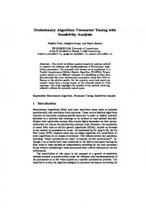
The winner is duplicated and overwrites the loser. Next, the second individual is selected and competes with a randomly chosen individual from the rest of the population excluding the first individual. This iterative procedure goes on until all the individuals have been considered. Figure 1 shows a complete selection of a vector population of five individuals. The shaded squares indicate the two competing individuals. In this experiment, and contrary to that in [1], the vector population is not reversed at the end of the selection so that the propagation of the fittest individual is slowed down.
In addition, for each chess piece captured and before the move is committed, a quiescence check operation is carried out. This process provides another 3 ply search.
By using this iterative method for selection, the fittest individual will ultimately occupy the last slot of the vector population.
The game is terminated when one of the three conditions is fulfilled: a checkmate state, no legal moves for a given player, or both players have reached 50 moves without winning. A player receives 1 point for a win and 0 for a draw or a loss.
B. Mutation In this experiment, a real-coded mutation operator is used as the main operator to tune the parameters of the evaluation function of each individual. We choose to use the polynomial mutation as devised in [11]. Its distribution parameterη is set to 20. The mutated parameter y is given below.
Where: Q, W = Quantity, Weight. Q [7] = {Q king, Q queen, Q rook, Q bishop, Q knight, Q pawn, Q double pawn, Q mobility} W [7] = {W king, W queen, W rook, W bishop, W knight, W pawn, W double pawn, W mobility}
III.
METHOD
We use an evolutionary algorithm to optimise the evaluation function. An individual is represented by a real vector of dimension 6. Each vector element represents the weight of either a chess piece other than the king and the pawn (which are assigned constant weights of 1000 and 1 respectively), a double pawn, or a mobility. There are five individuals in any given population. They all compete with each other for survival. Two individuals (two chess programs using two different evaluation functions) play each other in a two round game where each one will take turns in starting the game first. If an individual wins, it is awarded +1, otherwise 0. Based on the points collected from this tworound game, the winner is cloned and its clone mutated. Both the winner and its mutated version are copied into the next generation. This process continues until all individuals in the population converge to the same solution. A. Selection A vector population of five individuals is used where the selection process, a slight modification of the one in [1], is as follows. First we choose the first individual and make it compete with a randomly chosen individual from among the
(1,t +1)
yi The parameter
G
δi
G = x(i1,t +1) + ( xi(U ) − x(i L ))δ i
(2)
is calculated from the polynomial
probability distribution:
P(δ ) = 0.5(η m + 1)(1 − | δ |ηm)
(3)
(2r )1/(ηm +1) − 1, If r < 0.5 i i δi= 1/(η m +1) , If ri >= 0.5 1 − [2(1 − ri )]
(4)
Where: (1,t +1)
yi
x
(1,t +1) i (U )
xi
= new parameter after mutation = parameter before mutation
= parameter upper boundary
( L)
xi
= parameter lower boundary η = probability to mutate the parameter close to original parameter r = random number in [0 1]. Recall that each individual consists of six parameters denoting the weights of the different chess pieces (except the king and the pawn), double pawn and mobility. For each parameter, a specific value of its probability of mutation is assigned to it. For instance, the mutation probabilities for queen, rook, bishop, and knight parameters were all set to 25%, while the mutation probabilities for a double pawn and mobility parameters were set to 10%. Note that the mutation probabilities are relatively higher than the usual. This is to make sure that at least one parameter is mutated so that there will be no duplicated individuals in the population. C. Dy namic Boundary Strategy A good search method must promote diversity so that it is not trapped in a local optima. The search space in this application is very large. The diversity of a search method can be reflected by the standard deviations of each of the parameters. If the standard deviation is large then the diversity of the search method will be also large, whereas if the standard deviation is reduced, the diversity will also be reduced. To solve the problem of converging to a local optima, we propose a new approach called Dynamic Boundary Strategy. This strategy (at the same time) maintains and controls the diversity of the search throughout the generations. In other approaches [1], it is required to fix the upper and lower boundaries for each of the individual’s parameters. The basic idea of the dynamic boundary strategy is to have an adjustable boundary for each parameter. Consider the following individual with the initial parameters: Queen Rook Bishop Knight Double Pawn Mobility 9
5
3
3
0.5
0.1
The boundaries for the domain of each parameter are dynamic, however the diameter of that domain is constant. For instance, the diameters of the domains of the queen, the rook, the bishop, and the knight are all set to the value 2. The double pawn’s domain is set the value 0.2. The Mobility’ boundaries are fixed however (upper boundary =0.5, lower boundary =0.01). For instance, if the weight of the queen is 9, then its upper boundary is 11 and its lower boundary is 7. If the weight of double pawn is 0.5, then its upper and lower boundaries are respectively 0.7and 0.3. For example, the parameters of the above individual after applying the polynomial mutation could be as the following:
Queen Rook Bishop Knight Double Pawn Mobility 8.25
5
3
3
0.5
0.1
Notice that the weight of the queen has been mutated from 9 to 8.25. Then, the upper boundary of the queen will change to 10.25 while its lower boundary will become 6.25. This means that when the next mutation occurs on the queen’s weight, the possible weight for the queen will range from 10.25 to 6.25. In order to speed up the learning process, the weight of the queen can be forced to be at least equal to the highest parameter of the individual (such as rook, bishop, or knight). This is because it is sensible to think that the weight of the queen must be higher than the weight of any other chess piece (other than the king) as it is the most useful piece in a chess game. For example, consider the following values of the parameters of a given individual: Queen Rook Bishop Knight Double Pawn Mobility 4.5
5
3
3
0.5
0.1
Notice that the Rook’s weight is the highest. It is obvious that the Queen’s weight should be at least as higher as that of the Rook. Therefore, we can bring the Queen’s weight up to 5, which is now equal to the Rook’s weight. Queen Rook Bishop Knight Double Pawn Mobility 5
5
3
3
0.5
0.1
The main advantage of dynamic boundary strategy is that the search space in one generation of learning is much smaller compared to that of other fixed boundary strategies. Indeed, the dynamic boundary strategy explores small portions of the search space at each generation. However, in the long run, it is still capable of exploring a huge part of the search space. This is due to its moving boundaries. The main idea is that at each generation, the search process is concentrated in one part of the search space. Without this strategy, one needs to set good boundaries for the parameter’s domain, otherwise, a sufficiently large domain must be thought of, which is not a trivial task. This is not required when using the dynamic boundary strategy IV.
EXPERIMENTAL RESULTS
A. Experimental Design A small population of five individuals is used for breeding a good solution. The values for each of the parameters were inserted manually to make sure that the initial population only consists of poor individuals (bad evaluation functions). The purpose was to see whether the dynamic boundary strategy would be able to ameliorate the fitness (evaluation function) of the individuals. The initial individuals of the population are shown in Table I.
TABLE I.
THE INDIVIDUALS OF THE INITIAL POPULATION
Queen Rook Bishop Knight Individual 1 Individual 2 Individual 3 Individual 4 Individual 5
3 2.5 2 1.5 1
3 2.5 2 1.5 1
3 2.5 2 1.5 1
3 2.5 2 1.5 1
Double Mobility Pawn 0.5 0.1 0.5 0.1 0.5 0.1 0.5 0.1 0.5 0.1
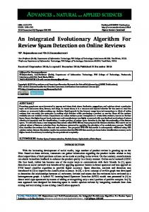
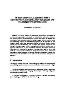
Recall from the section II that our chess program was designed to search 3 ply and we can extend the search another 3 ply when the quiescence check operation is triggered. We run the program for 520 generations. The means and the standard deviations of the initial population are given below in Table II. B. Results After learning for 520 generations, the values of the parameters of the individuals have changed a lot. Figure 2 and Figure 3 respectively show the averages and the standard deviations of the parameters throughout the whole learning procedure (520 generations). The averages of the weights and their standard deviations at the end of the experiments are given in Table III. It is worth noting that in evolutionary algorithms that use a fixed boundary approach, the diversity of the search decreases gradually after many generations. Notice also that the standard deviations of the last population (using our strategy) shown in Table III have not changed too far from their initial standard deviations counterpart (shown in Table II). C. Success The weights of the Shannon’s evaluation function [5] are as follows:
TABLE III.
AVERAGES AND STDEVS AT THE LAST POPULATION.
Queen Rook Bishop Knight Average STDEV
7.60 0.08
3.86 0.68
5
3
3
0.5
0.1
After running our chess program for 520 generations, the learning process produced the fittest individual whose parameter values are as follows Queen Rook Bishop Knight Double Pawn Mobility 7.57 TABLE II.
4.66
4.41
3.16
0.44
In the first game, the chess program based on the Shannon’s evaluation function dominated the game, but the game ended with a draw because both players have reached the 50 move limit. However, in the second game, the fittest individual of our chess program took control of the game and ended it in just 42 moves (21 moves for each player). This result has shown that the fittest individual is strong enough to win against a wellestablished evaluation function. We further tested our chess program based on the dynamic boundary strategy against a well-known commercial chess program called “Chessmaster 8000”. The Chessmaster 8000 level of difficulty was set to players rating 1800, which falls in the A class in the USCF rating. The fittest individual of our chess program played as White player for two games and the results are shown in Table V. In the first game, the Chessmaster 8000 beat the fittest individual in 81 moves. We consider this as a promising result as our fittest individual was competitive enough to last this long. The second game ended with a draw because of the 50 move limit. However, our fittest individual did very well in this round as it was dominating the game, and had the game been extended, it would have beaten the ChessMaster 8000. Our chess program was left with a rook and a pawn, while the Chessmaster 8000 was left with 2 pawns only. CONCLUSION In this paper, we have proposed the use a novel approach for the evaluation function of a chess playing game. This is called Dynamic Boundary Strategy This method is quite effective because those parts of the search space that are not promising would not be visited. However, it is important to make sure that the diameter of the interval (distance between upper and lower boundary) of the weight of a given parameter must be large enough so that the
AVERAGES AND THE STDEVS AT THE INITIAL POPULATION
Queen Rook Bishop Knight Average STDEV
0.11
2.95 0.12
This fittest individual was tested against a chess program that uses the Shannon’s evaluation function. The results are shown in Table IV.
Queen Rook Bishop Knight Double Pawn Mobility 9
3.56 0.69
Double Mobility Pawn 0.48 0.10 0.03 0.01
2 0.71
2 0.71
2 0.71
2 0.71
Double Mobility Pawn 0.5 0.1 0.0 0.0
TABLE IV.
FITTEST INDIVIDUAL AGAINST SHANNON’ EVALUATION FUNCTION.
Fittest Individual Fittest Individual
Play as White Black
Moves 100 moves 42 moves
Result Draw Win
The Average of each Evaluation Parameter in the Population
6 5
Weight
4 3 2 1
520
500
480
460
440
420
400
380
360
340
320
300
280
260
240
220
200
180
160
140
120
100
80
60
40
20
0
0 Generation Queen
Rook
Bishop
Knight
Double Pawn
Mobility
Figure 2. . Averages of each parameter throughout the learning process
The Standard Deviation for each Evaluation Parameter in the Population
Standard Deviation
2.5 2 1.5 1 0.5
51 0
48 0
45 0
42 0
39 0
36 0
33 0
30 0
27 0
24 0
21 0
18 0
15 0
12 0
90
60
30
0
0
Generation Queen
Rook
Bishop
Knight
Double Pawn
Mobility
Figure 3. Standard deviations of each parameter throughout the learning process
search is not trapped into a local optima. The fittest individual produced by our method is still unable to compete against a very good chess player (Chessmaster 8000), but it has proven that the learning algorithm was able to optimise (to some extent) the evaluation function that is used to determine a good move. It has beaten the chess program that uses Shannon’s evaluation function. In our future work, we will extend the search depth, to
incorporate heuristics, and use a more complex evaluation function. This, we hope, will produce a very competitive chess playing individual.
TABLE V.
FITTEST INDIVIDUAL AGAINST CHESSMASTER 8000.
Fittest Individual Fittest Individual
Play as White White
Moves 81 moves 100 moves
Result Lost Draw
APPENDIX st
1 game: Fittest Individual (White) Vs. Chessmaster 8000 (Black) 1 e2e3 g8f6 26 a1a4 c8f5 2 f1d3 d7d6 27 h1b1 b7b5 3 d1f3 h8g8 28 b1b5 f5h3 4 b2b3 b8d7 29 g2h3 e7f6 5 b1c3 h7h5 30 c3f6 a6b5 6 f3f5 a7a6 31 a4a8 e8d7 7 g1f3 c7c5 32 h3h4 d7e6 8 h2h3 e7e6 33 a8c8 e6f6 9 f5f4 f6d5 34 h4h5 f6e6 10 c3d5 e6d5 35 h5h4 e6e7 11 f4f5 d8c7 36 e3e4 b5b4 12 c1b2 d7f6 37 c8c7 e7f6 13 f5f4 f6e4 38 h4g3 f6e5 14 a2a4 g7g5 39 c7e7 e5d4 15 f3g5 g8g5 40 g3g2 b4b3 16 f2f3 c7a5 41 g2g3 b3b2 17 a1d1 g5g2 42 e7b7 d4e4 18 f3e4 c5c4 43 b7b2 f7f5 19 e1f1 f8e7 44 b2b4 e4d5 20 f1g2 c4d3 45 g3g2 f5f4 21 b3b4 a5b4 46 b4f4 d5e5 22 b2c3 b4a4 47 f4f7 e5d5 23 d1a1 a4e4 48 f7f6 d5c5 24 f4e4 d5e4 49 f6f7 c5d5 25 c2d3 e4d3 50 g2g3 d5c5 2nd game: Fittest Individual (White) Vs. Chessmaster 8000 (Black) 1 e2e3 g8f6 26 d2e3 f4g5 2 f1d3 d7d6 22 h1g1 d8h4 3 d1f3 h8g8 23 g1h1 d5e4 4 b2b3 b8d7 24 d3c4 e4e3 5 b1c3 h7h5 25 h1h2 h4f4 6 f3f5 a7a6 27 g2h1 g5e7 7 g1f3 c7c5 28 h1g2 e7e4 8 h2h3 e7e6 29 g2f1 c8e6 9 f5f4 f6d5 30 c4e2 e4e3 10 c3d5 e6d5 31 b2c1 e6h3 11 f4f5 d8c7 32 h2h3 e3h3 12 c1b2 d7f6 33 f1f2 h3h4
13 14 15 16 17 18 19 20 21
f5f4 a2a4 f3g5 f2f3 f3e4 a4a5 e1f1 f1g2 e3f4
f6e4 g7g5 g8g5 g5g2 c7b8 b8c7 f8h6 h6f4 c7d8
34 35 36 37 38 39 40 41
f2f1 c1e3 f1g2 e2h5 g2f3 f3e4 e4d5 d5d6
e8c8 h4f6 f6a1 d8g8 a1f1 g8e8 e8e5
ACKNOWLEDGMENT The author Hendra Suhanto Poh thanks Nasa Tjan for his assistance in developing the chess engine, and Gunawan for providing a facility to run the experiments. REFERENCES [1]
G. Kendall and G. Whitwell, “An evolutionary approach for the tuning of a chess evaluation function using population dynamics,” Proceedings of the 2001 Congress on Evolutionary Computation, vol. 2, pp. 9951002, May 2001. [2] G. Whitwell, “Artificial Intelligence Chess with Adaptive Learning,” Bachelor Degree Dissertation Thesis, the University of Nottingham, May 2000. [3] D. B. Fogel, T. J. Hays, S. L. Hahn, and J. Quon, “A self-learning evolutionary chess program,” Proceeding of the IEEE, vol. 92, Issue 12, pp. 1947-1954, Dec. 2004. [4] D. Kopec, M. Newborn, and M. Valvo, “The 22d annual ACM international computer chess championship,” Communication of the ACM, vol. 35, Issue 11, pp. 100-110, Nov 1992. [5] E. Shannon, Claude, “XXII. Programming a Computer for Playing Chess,” Philosophical Magazine, Ser. 7, vol. 41, No. 314, Mar 1950. [6] Z. Michalewicz, “Genetic algorithms + data structures = evolution programs / Zbigniew Michalewicz,” Berlin: Springer-Verlag, 3rd Edition revised and extended, 1996. [7] S. J. Russel and P. Norvig, “Artificial Intelligence: A Modern Approach,” Upper Saddle River, N.J.: Prentice Hall/Pearson Education, 2nd Edition, 2003. [8] D. Goldberg, “Genetic Algorithms in Search, Optimization, and Machine Learning/ David E. Goldberg,” Boston, Mass.: Addison, Wesley, 1989. [9] H. Kaindl, “Tree searching algorithms,” in Computers, Chess, and Cognition, T. A. Marsland and J. Schaeffer, Eds. New York: SpringerVerlag, pp. 133–168, 1990. [10] F. G. Luger, “Artificial Intelligence: Structures and Strategies for Complex Problem Solving,” Addison Wesley Publishing Company, 4th Edition, p. 144 – 152, 1997. [11] K. Deb and K. B. Agrawal, “Simulated Binary Crossover For Continuous Search Space.” Complex System , vol 9, pp.115-148, 1994.